a sub-swarm is created by grouping the particles that are closer to the best solution. The basic PSO algorithm was developed to find unique solutions to optimization problems, some variations of PSO are to solve problems such as multi objective optimization, dynamically changing objective functions and location of multiple solutions.
A variation of PSO are techniques of niches. The NichePSO algorithm was developed by Bris et al. [1]. It em-ploys PSO to find multiple solutions to multimodal problems. It was the first PSO niching technique that introduces a novel PSO algorithm to detect multiple optimal in a multimodal problem whose implementation can be parallelized. The particle swarm concept was to simulate the graceful of choreography of a bird flock, that govern the ability to fly synchronously and suddenly chance direction or velocity. The position of particles are based on the social psycho-logical tendency of individuals to emulate other individuals, and is given by
xi(t+ 1) =xi(t) +vi(t+ 1) (1)
wherevi(t)denotes the velocity vector or the i-th particle. The velocity update has the form:
vij(t+ 1) =vij(t) +c1r1j(t)pij(t) +c2r2j(t)sij(t) (2)
where the subindex ij denotes dej-th entry corresponding toi-th particle, andp(t)is the cognitive component ands(t)
the social component, c1 and c2 are positive acceleration constants used to the contribution of the cognitive and social components,r1j andr2j are random values from a uniform distribution U[0,1]. Each step t a particle i updates its velocity and position, were the new velocity vi(t+ 1), is the sume of three terms, the previous velocity vi(t), to the distance fromlbestand the best position particle fromgbest. The PSO is in Algorithm 1 where the first step for PSO algorithm is the initialization of the main swarm, where cognitive component, social component, position and velocity need to be specified, in line 3 the fitness function is evaluated for each particle. In line 11 and 12 the position and velocity are updated; this process is repeated until a stopping condition is satisfied.
Algorithm 1 PSO Algorithm
1: Create and initialize annx-dimensional swarm;
2: repeat
3: foreach particle i= 1, ..., ns do 4: if f(xi)< f(yi)then
5: yi=xi;
6: end if
7: if f(yi)< f(ˆyi)then 8: yˆ=yi
9: end if
10: end for
11: foreach particle i= 1, ..., ns do 12: update the position using equation 1; 13: update the velocity using equation 2;
14: end for
15: untilstopping condition is true;
B. NichePSO
A PSO based algorithm called NichePSO assumes as an objective to find the different maxima of the problem. NichePSO updates the best particle position and velocity while also using PSO for the rest of the particles. The updating formulae are as follows
xrj(t+ 1) =yj(t) +wvrj(t) +p(t)(1−2r2(t)) (3)
vrj(t+1) =−xrj(t)+yj(t)+wvrj(t)+p(t)(1−2r2(t)) (4)
The NichePSO algorithm is the one presented in Algo-rithm 2.
Algorithm 2NichePSO Algorithm
1: Create and initialize a nx-dimensional main swarm, S;
2: repeat
3: Train the main swarm, S, for one iteration using the cognition-only model;
4: Update the fitness of each main swarm particle,S.xi; 5: foreach sub-swarmSk do
6: Train sub-swarm particles,sk.xi using a full model PSO;
7: Update each particle’s fitness; 8: Update the swarm radius Sk.R;
9: end for
10: If possible, merge sub-swarms;
11: Allow sub-swarms to absorb any particles from the main swarm that moved into the sub-swarm;
12: If possible, create new sub-swarms; 13: untilstopping condition is true
14: return Sk.yˆfor each sub-swarmSk as a solution;
The initialization of the main swarm is done in line 1. In line 3 this swarm is trained with the cognitive model only. In line 4 the fitness function for each particle is updated, then in line 6 the sub-swarms are trained using a PSO full model, after updating the fitness for each particle in line 7, in line 8 the swarms radius are update. In line 10, the sub-swarms are merged if is possible. Finally the best particle of each sub-swarm is returned as a solution in line 14.
The NichePSO has good performance when finding the solutions to multimodal problems. However, it was found that the current sub-swarm merging and particle absorption strategies are premature, and limits exploration in the main swarm. That is shown in [10] where they describe original merging and absorption routines within the NichePSO. This can be enhanced by including behavioral information in the decision making process whether to merge or not. They proposes four new strategies, two for enhanced merging (Directional Based Merging and Scatter Merging) and two for enhanced absorption (Directional Based Absorption and Euclidean Diversity Absorption).
III. BIFURCATIONDIAGRAMS
number of solutions of the equation f(x;θ) = 0 for x in every neighborhood of(x0, θ0)is not a constant independient of θ.
A Bifurcation Diagram (BD) is the generation of a graph which explicitly tell us about the dynamics of the equation roots as its parameters are continuously changing. Each of this points can then be evaluated for their stability assess-ment, for which there exist several well stablished methods and therefore are left out of this work as does not add anything new. An example of a one dimensional BD [9] is the equation 5:
˙
x=θx+x3−x5 (5)
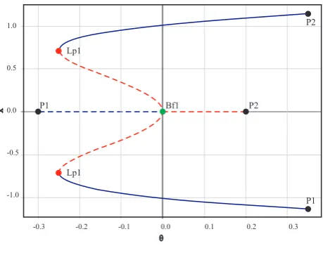
has a subcritical pitchfork bifurcation at (x, θ) = (0,0). When solutionx= 0loses stability asθpasses through zero, the system can jump to one of the distant stable equilibria corresponding to x=±1 atθ= 0.
1.0
0.5
0.0
-0.5
-1.0
-0.3 -0.2 -0.1 0.0 0.1 0.2 0.3
x
θ Lp1
P2
P2
P1
P1 Bf1
[image:3.595.56.286.260.445.2]Lp1
Fig. 1. Bifurcation Diagramxt=θx+x3−x5
Figure 1 represents a BD whereθis the parameter which will be changing and therefore the equation roots will be probably also changing. Here, we can observe that whenθ=
−0.25a two bifurcation points were found one atx=−0.7
and the other at x = 0.7, moreover, these two bifurcations appear (or disappear if we were diminishing θ), please do notice we now have three roots, instead of one which we had if we go back an infinitesimal distance fromθ=−0.25. We can also observe that if we increase by an infinitesimal valueθ, we will have five roots. Another interesting point is when θ = 0 where before reaching that value we had five roots and in that value three roots merge to just one root e.g
x= 0.Bf1point is the bifurcation,LP1are turning points or limit points, P1,P2andLP1 are branch points.
IV. PROPOSEDMETHODOLOGY
Torres et al. [9] describe the normal NichePSO algorithm is constantly applied to build the BD but the previous solution to the problem is ignored, which makes it a slow process. The methodology we propose takes the previous solution as a starting point to find the following solution. This poses two additional problems which can arise along the bifurcation diagram generation process: Appearance of new roots and disappearing of existing roots. To this end, we are proposing new heuristics in order to deal with them. In the following section we will describe the main concepts of our methodology.
A. Problem Transformation
PSO as well as NichePSO were designed to deal with op-timization problems, however in order to find the bifurcation diagram we need to find the zeroes of the system. To this end, we need to transform our dynamic system functionf into a functiong where all the zeroes will be the maximal points of the transformed function g. Specifically, g is defined as equation 6.
g(x) = 1
1 +kf(x)k (6)
This function will be the one we will use to evaluate the fitness of the elements of the swarm.
B. Bisections Method
Traditionally, the bisection method [12] has been used as a means to find the root of a given function. This method iteratively converges on a point where f(x) = 0 which is taken as the solution of the process. It basically changes a reference point, x, at the middle of the space search i.e. [xa..xb] and the deciding which of the halves to explore i.e. [xa, x] or [x, xb] based on some criteria. Usually this criterion is the sign of the function evaluated at x, xa, xb. In our method our criterion will be the number of roots at
x, xa, xb. In this contribution we will use this method as a mean to find the bifurcation point. This process will be called when, as a result of the NichePSO application, a different number of roots, from those we were processing, are found. The bisection method in our case is illustrated in Figure 2 where we can see, when NichePSO is applied, a different number of roots at the ends of the green range. This fact will fire the bisection process which moves the reference point at the middle of the green range and now decides to search the blue range as it is there where a different in the number of roots are present at the limits of this range. This process will go on until, ifxn is the bifurcation point,|xn−xn−1|< .
1.0
0.5
0.0
-0.5
-1.0
-0.3 -0.2 -0.1 0.0 0.1 0.2 0.3
x axis
[image:3.595.320.533.504.657.2]θaxis
Fig. 2. Bisection Method
C. The fastBDPSO algorithm
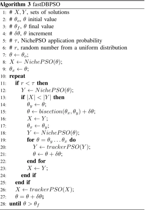
The main algorithm proposed in this work is shown in algorithm 3. Line 8 calls NichePSO which returns a set of solutions which are stored in X. Then we will repeat the following process. If stochastically determined, apply NichePSO() (line 12) and if the number of solutions are greater from those in X, the bisection method is applied to find the bifurcation point (line 15). NichePSO is called again after that point θ+δθ (line 18). From that point we will apply the trackerPSO algorithm to follow the track of each solution from θx toθy (lines 19-22). Please do notice that in this tracking process NichePSO will not be called again. Line 26 will call trackerPSO to follow the solutions path and finally in line 27 θ is increased. This process will be repeated untilθ > θf.
Algorithm 3 fastDBPSO
1: #X, Y, sets of solutions 2: #θo,θ initial value 3: #θf,θ final value 4: #δθ,θ increment
5: #τ, NichePSO application probability
6: #r, random number from a uniform distribution 7: θ←θo;
8: X←N icheP SO(θ); 9: θx←θ;
10: repeat
11: ifr < τ then
12: Y ←N icheP SO(θ); 13: if |X|<|Y|then
14: θy ←θ;
15: θ←bisection(θx, θy) +δθ;
16: X ←Y;
17: θx←θy;
18: Y ←N icheP SO(θ); 19: forθ=θy. . . θx do
20: Y ←trackerP SO(Y);
21: θ←θ+δθ;
22: end for
23: X ←Y;
24: end if
25: end if
26: X←trackerP SO(X); 27: θ=θ+δθ;
28: untilθ > θf
On the other hand the trackerPSO algorithm is described by algorithm 4, This heavily relies on PSO, the only difference being in the initialization part where the best particle becomes the previous solution of that path and a five particles swarm is created around such particle (line 3). This will be done for every particle of the solution passed to trackerPSO (X). It is worthy to note that in this case the social component will be highly more important that the cognitive component therefore in the PSO algorithm the following must be fulfilledC1<< C2.
V. EXPERIMENTALRESULTS
NichePSO is computationally expensive, for this reason this is only employed in case it is needed and we heavily rely on tracking previous solutions using simple methods
Algorithm 4trackerPSO(X)
1: # X, sets of solutions 2: foreach x∈X do
3: xs←Create a five particles biased swarm around x; 4: y←P SO(xs);
5: mergeSolutions(); 6: end for
i.e. PSO and DE. The main difference is that we use fewer particles to follow such solutions as the previous solution has to be very close to the one we are looking for. Therefore, the efficiency as well as the precision is improved. This section show some experiments in relation with time response as well as accuracy for several systems. The experiments were conducted on an laptop computer MacBook Air, 4 Gb RAM, 1600 MHz DDR3, 1.6 GHz Intel Core i5, using macOS Sierra version 10.12.5. To render the results a bifurcation di-agram plotting tool, called BDT (Bifurcation Didi-agram Tool), was implemented. In these experiments some parameters were measured, these are: time for creating the bifurcation diagram, precision to find the roots, the minimum number of particles necessary for good performance, apply NichePSO (BD-NichePSO), and track with PSO (Fast BD-PSO) as well as DE (FAST BD-DE).
The first column of Table I shows all the used parameters as well as nd a determinate iterations number for each test.
TABLE I
NICHEPARAMETERSSETTING
Parameters Niche Fast BD-PSO Fast BD-DE
Main Swarm Size 40, 65, 130 & 260 5 5
Learning FactorC1 1 0.8
-Learning FactorC2 2 2
-Inertia weightW 0.5 0.5 0.4
Cross Rate - - 0.8
Iteration number 65 30 30
With the purpose of comparing the efficiency a mod-ified version of fastBDPSO implemented , where instead of using PSO in the tracking algorithm (line 4, algorithm 4) we use differential evolution which will be called Fast BD-DE. We have as reference the algorithm which uses NichePSO along all the different values of θ, which will be called simpleNichePSO. We also test the cases for
[image:4.595.48.293.235.589.2]δθ = 0.1,0.01,0.001 steps for the three algorithms i.e. simpleNichePSO, fastBD-PSO and fastBD-DE algorithms using the same equation in a one dimensional diagram. Figure 3 shows the results of the different methods when applied to function f( ˙x, θ) = θx+x3−x5. All the cases were able to generate the BD, but as later will be shown, fastBDPSO outperforms the other two algorithms.
x axis
θaxis
[image:5.595.59.281.58.336.2]0.1 Steps for experiments 0.01 Steps for experiments 0.001 Steps Bisection Method
Fig. 3. Test withf( ˙x, θ) =θx+x3−x5
1.0
0.5
0.0
-0.5
-1.0
-0.3 -0.2 -0.1 0.0 0.1 0.2 0.3
x axis
θaxis
(a) 5 Particles
1.0
0.5
0.0
-0.5
-1.0
-0.3 -0.2 -0.1 0.0 0.1 0.2 0.3
x axis
θaxis
(b) 8 Particles
Fig. 4. Particle Tracking with 5 and 8 particles.
Table II shows some tests performed for all functions shown in first column. The second column show the value ranges for the functions. The third column shows the step size, and the last columns show the time required buy simpleNichePSO to obtain the BD with different number of particles i.e. 40, 65, 130 and 260. Elements in red were not able to generate the BD, therefore a swarm of 130 particles was decided to be used for simpleNichePSO.
TABLE II
NICHEPSOFOR DIFFERENT NUMBER OF PARTICLES
Function Ranges Step Niche
40 65 130 260
x= (−1.4,1.4) 0.1 0.6722 0.9336 1.6120 2.8532
−x5+x3+xθ θ= (−0.32,0.25) 0.01 5.6544 7.6904 13.2951 23.5480
0.001 54.3783 76.2523 125.6771 219.5866
x= (−4,4) 1 1.4843 1.7264 2.5844 4.54245
4x−x3+θ θ= (−4,4) 0.1 11.9331 14.7582 22.0439 36.9021
0.01 115.3369 141.7751 210.6229 334.1761
x= (−10,10) 1 6.0179 6.4065 8.3627 12.0327
x+θ−x2 θ= (−10,10) 0.1 54.0352 58.5006 77.8289 115.5978
0.01 506.0416 546.2896 712.4901 1034.6116
Figure 5 shows the results of the experiments using the functions and methods there described.
TABLE III PARTICLESTRACKINGTIME
Function Step Fast BD-PSO Fast BD-DE Niche
0.1 8.2676 17.7030 1.6120
−x5+x3+xθ 0.01 9.0056 20.443915 13.2951
0.001 22.7764 52.292652 125.6771 1 76.2738 151.0828 2.5844 4x−x3+θ 0.1 79.3385 155.2536 22.0439
0.01 81.1868 168.5666 210.6229
1 77.3132 160.3031 8.3629
x+θ−x2 0.1 70.7938 158.2267 77.8289
0.01 78.4142 174.9785 712.4901
As it can be seen, there is a Difference of time in tracking between Fast BD-PSO and Fast BD-DE. This was related
(a) Original Diagram (b) NichePSO
(c) Fast BD-PSO (d) Fast BD-DE
Fig. 5. Results for−x5+x3+xθFunction
to the heuristic of the PSO algorithm which is based on repulsion between particles with umbral to generate all the candidates around a point. Therefore, it is forced to converge faster using best position which is the solution to that path in the previous iteration. Tracking with Fast BD-DE algorithm the basic idea is the same to the previous case, but now mu-tation functions were used as well as the recombination that characterizes this algorithm. Consequently more iterations are needed to converge directly affecting the performance. The tracking of the particles is shown in Table III. As we can see the computational time for fastBD-PSO is half the time used by fastBD-DE in all cases and in general it outperforms simpleNichePSO.
VI. CONCLUSIONS ANDFUTUREWORK
REFERENCES
[1] R. Brits, A. P. Engelbrecht, and F. Van den Bergh, “A niching particle swarm optimizer,” inProceedings of the 4th Asia-Pacific conference on simulated evolution and learning, vol. 2. Singapore: Orchid Country Club, 2002, pp. 692–696.
[2] B.-Y. Qu, P. N. Suganthan, and S. Das, “A distance-based locally informed particle swarm model for multimodal optimization,”IEEE Transactions on Evolutionary Computation, vol. 17, no. 3, pp. 387– 402, 2013.
[3] S. Bird and X. Li, “Adaptively choosing niching parameters in a pso,” inProceedings of the 8th annual conference on Genetic and evolutionary computation. ACM, 2006, pp. 3–10.
[4] I. Schoeman and A. Engelbrecht, “Using vector operations to identify niches for particle swarm optimization,” inCybernetics and Intelligent Systems, 2004 IEEE Conference on, vol. 1. IEEE, 2004, pp. 361–366. [5] X. Li, “Adaptively choosing neighbourhood bests using species in a particle swarm optimizer for multimodal function optimization,” in
Genetic and Evolutionary Computation Conference. Springer, 2004, pp. 105–116.
[6] G. Cheng, Y. An, Z. Wang, and K. Zhu, “Oil well placement opti-mization using niche particle swarm optiopti-mization,” inComputational Intelligence and Security (CIS), 2012 Eighth International Conference on. IEEE, 2012, pp. 61–64.
[7] L. Menezes and A. L. Coelho, “On ensembles of biclusters gener-ated by nichepso,” inEvolutionary Computation (CEC), 2011 IEEE Congress on. IEEE, 2011, pp. 601–607.
[8] H. T. Yao, H. Q. Chen, and T. F. Qin, “Niche pso particle filter with particles fusion for target tracking,” inApplied Mechanics and Materials, vol. 239. Trans Tech Publ, 2013, pp. 1368–1372. [9] O. V. Torres, J. C. Jacobo, and J. J. Flores, “A bifurcation diagram tool
based on nichepso,” inPower, Electronics and Computing (ROPEC), 2013 IEEE International Autumn Meeting on. IEEE, 2013, pp. 1–5. [10] A. P. Engelbrecht and L. Van Loggerenberg, “Enhancing the nichepso,” inEvolutionary Computation, 2007. CEC 2007. IEEE Congress on. IEEE, 2007, pp. 2297–2302.
[11] T. Zhou, Bifurcation. New York, NY: Springer New York, 2013, pp. 79–86. [Online]. Available: https://doi.org/10.1007/ 978-1-4419-9863-7 500