The Uncertainty Reduction for the Refined Sample Mean of Combined Quantities

The Uncertainty Reduction for the Refined Sample Mean

of Combined Quantities

Abstract—Sampling plans for middle or small sample size are often taken when the available data is not large enough. In this paper, a new quantile-based maximum likelihood estimation (QMLE) method for mean value estimation of a quasi-normal distribution is proposed. It takes the two endpoints of range as quasi-symmetric quantiles and fuses the concept of empirical and symmetric quantiles to define an objective function. It then follows the well-known “asymptotic minimax principle”, which is a robust statistical method, to realize the optimization of the objective function. Simulation results confirmed that the proposed QMLE mean estimator outperforms the conventional sample mean estimatorwith about 40% uncertainty, or mean square error (MSE), reduction.

Index Terms—sample mean, maximum likelihood estimation, quantile, combined quantities, asymptotic minimax principle

I. INTRODUCTION

There are some signals that are not strictly conforming to normal distribution, but still behaving like normal distribution. We call them quasi-normal signals. A typical example of signal of this style is the hybrid output of combining several different quantities which are submitted to normal, rectangular, triangular or Student’s t-distributions. Up till now, it is convenient and popular to apply Law of Uncertainty of Propagation [1] to model the standard uncertainty for the combined quantities. But it still lacks a formulation to describe the mean value of the combined quantities except the sample mean. In this study, we are interested in the mean value estimation for combined quantities conditioned on middle or small sample size. We would like to use the normal estimator to estimate the mean value of quasi-normal data.

A general form of hybrid signal of combined quantities can be expressed as

1 1 2 2 n n

x c z= +c z +_LLc z (1)

where is the i-th input quantity and is the corresponding weight. Fotowicz [2,3] gave a brief description about the quantization of uncertainty of combined quantities for the case that there is at least one input quantity conforming to the rectangular distribution. The weighted sum output can be approximated by an R*N distribution, which is the convolution of a rectangular function and a normal distribution.

i

z ci

Wen-Hui Lo is with the Department of Communications Engineering, National Chiao Tung University Hsinchu, Taiwan 30050, email: [email protected]

Prof. Sin-Horng Chen is with the Department of Communications Engineering, National Chiao Tung University, Hsinchu 30050, Taiwan..

.

The shape of R*N distribution depends on the uncertainty ratio (UR) expressed by

2 2

[ ( )]

( ) [ ( )]

i

c i

Max u x UR

u x Max u x

=

−

(2)

where is the standard uncertainty of the i-th input quantity which is rectangular distributed, and is the combined standard uncertainty. An example of R*N pdf is given as

( )

i

u x

( )

c

u x

( )

2

+ 3 2 3

1 ( )

2 6

u u

t

x r

RN _{x r}

c

f x e

K π UR

−

−

=

_∫

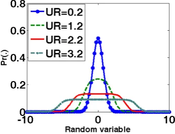
dt (3)

where is a normalization constant. Fig.1 displays the R*N pdf for several values of UR. is the shape parameter.

c

K

[image:1.595.340.514.393.526.2]

u

r

Fig. 1: Zero mean of R*N distribution for different uncertainty ratio (UR) In the past, sample mean is widely used in the mean value estimation for any signal no matter what its original pdf is. The main reason of using sample mean is that it is not only a uniformly minimum variance unbiased estimator (UMVUE) but also the random variable of central limit theorem (CLT). Bowen [4] has pointed out that CLT may be explained as the sum of independent variables with the characteristic function formed by the product of the component characteristic functions. If we can discard the unbiased requirement, there exist some biased estimators that outperform sample mean. Stearls [5] and Gleser [6] discussed a new approach for the given coefficients of variation of sample mean. Ashok et al. [7] further proposed a realistic method to adjust the coefficients of variation of sample mean to improve its performance.

Up till now, if we want to predict the mean value of combined quantities accurately, the only way is to take the sample mean on heavy observations. In practical applications of Measurement, the basic volume required for one digit

accuracy is observations for 95% coverage interval [8]. Sometimes, there are not enough samples to support this rule so that the middle or small sample size sampling plans are also often taken. Besides, the good property of UMVUE for sample mean may be ineffective for the case of combined quantities which is of quasi-normal distribution. This is because the property of UMVUE is derived from the maximum likelihood estimation (MLE) basing on the normal pdf assumption.

6 10

In this paper, a new method of mean value estimation, referred to as the quantile-based maximum likelihood estimator (QMLE), is proposed. The classical application of quantiles is the general usage of empirical quantiles. Koenker and Bassett [9] extended the empirical quantiles to the regression quantiles, which is specially useful for predicting the bounding information. Gilchrist [10] collected many studies about the estimation, validation, and statistical regression with quantile models. In the single quantile application, Giorgi and Narduzzi [11] gave the quantile estimation for the self-similar process. Heathcote, et al. [12] addressed the quantile maximum likelihood estimation of the response time distribution. But it involved a time-consuming numerical computation for the inverse of the quantile function, which is typical the cumulative distribution function (cdf) of normal pdf.

In the proposed QMLE, the quantiles are determined by the maximum percentage of population, i.e. coverage, so that it is composed of a couple of quasi-symmetric quantiles (QSQ). According to the past studies, the coverage-constrained quantiles will obey the properties of symmetric quantiles whose variances asymptotically approach to the Cramer-Rao lower bound [13]. The symmetric quantiles were described with strict definition given in [13]. But we consider it with a more flexible operation as the ranked variables of the first order sample x_1:n

and the last order sample xn n: . Hence the QSQ we considered are both empirical quantiles and quasi-symmetric quantiles. Lo and Chen [14,15] also derived good quantile-based estimators for the sparse data condition. In this study, we plan to derive the QMLE basing on the order statistics and expect that it can support not only the concept of empirical quantiles but also the quasi-symmetric quantiles. Otherwise, we would still need a quantile function defined below to link quantiles and MLE:

( ) Pr( _p)

Q p ≡ X ≤x = p (4) here, the value xp is called the p-quantile of population.

The paper is organized as follows. Section II presents the proposed QMLE. Section III establishes the minimax structure to realize the QMLE. Section IV suggests an advanced refinement of the QMLE to improve its performance. Some conclusions are given in the last section.

II. THE PROPOSED QUANTILE-BASED MEAN ESTIMATOR

We derive the QMLE by solving the problem of maximizing the objective function QMLE( , )μ σ defined by

2 2 1

: :

( )

( , ) ( log 2 log )

2 2

. for 1 or

n i i

p n p n

x n

QMLE n

x p n

μ

μ σ π σ

σ

μ σξ

=

⎧ −

= − − −

⎪ ⎨

⎪ = − =

⎩

∑

₍₅₎

where xp n: is the minimum order (for p=1) or maximum order (for p=n) of samples xi, 1≤ ≤i n; ξp n: is a standard normal random variable normalized from xp n: ; and n is the sample size. The solution derived in detail in Appendix is given below:

* :

* :

p xp n p p n

μ = −σ ξ (6) where

(

)

(

)

(

)

: :

*

2 ₂

: : :

1

( )

2

( ) 4 ( ( )

2

p n p n

p

n

p n p n i p n

i

n x x n

n x x n x x

n

ξ σ

ξ

=

− =

− + −

±

∑

) (7)

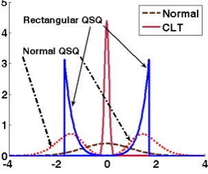
[image:2.595.357.509.426.553.2]

with the constraint _σ* _>0, and _{x is the sample mean.} If we emulate the pdf of combined quantities as a quasi-normal distribution (see the example shown in Fig. 1), one of its two extreme shapes looks like a rectangular pdf for large UR. Examining the first order and last order random variables (i.e. QSQ) of the rectangular and normal pdfs with the same standard uncertainty, we find that the dispersion-areas of QSQ of the rectangular pdf are more concentrated than the normal pdf.

Fig. 2: Standard normal pdf combined with its CLT pdf and QSQ pdf for sample size=11. We plot the QSQ of equal variance rectangular pdf

[− 3, 3] as the blue solid line.

III. ESTABLISH THE MINIMAX STRUCTURE

We then follow the well-known robust statistical method “asymptotic minimax principle” to realize the QMLE. Huber [16] ever addressed the robust statistical method via the least possible variance searching algorithm given below:

Asymptotic minimax results [16]: Let be a convex

compact set of distribution F on the real line. To find a sequence of estimators of location which have a small asymptotic variance over the whole of ; more precisely, the supremum over

κ

n

T

κ

κ of the asymptotic variance should be least possible.

searching algorithm. They are the convex set, least variance and a minimax optimization objective function. We describe them in detail in the following:

A. Convex set

Eq.(5) is a quadratic equation so that its global extreme does exist. According to this property, we construct the convex set comprising the candidates of population mean.

Using three normal pdfs, , and

as examples, we form their convex sets by using Eqs.(6) and (7). There are 1,000 trials with 15 samples in each trail. For each trial, the 15 samples are firstly sorted in the ascending order to find the two endpoints

2 (10,1 )

N _{N(2.3,0.8 )}2 2

(3.7,1.2 ) N

1:n

x and x_{n n:} . They are then transformed into the standard normal distributed versions, ξ1:n and ξn n: , by using a pre-assumed pseudo mean μps and the true standard deviation σ if it is

known (or the samples’ standard deviation 2

1

1 n _{( )}

s i

i

x x n

σ

=

=

∑

− ). Then, the estimate _σ* _{is calculated} by Eq.(7). We denote it as *

p

σ . The final mean estimate is obtained by Eq.(6), i.e., * *

: :

p p n p p n

u =x −σ ξ for p=1 or n. To evaluate the performance of the QMLE estimator, an averaged mean square error (MSE) defined by

(

* 2 * 2

)

1000 1 1

( ( ) ) ( ( ) )

1

1000 2

ps n ps

i

i i

MSE μ μ μ μ

=

− + −

=

∑

(8)

is calculated for each test. We take the error between the pseudo mean and real mean,

(

μ_ps−μ

)

, as the reference. We set the inspection interval of μps to be

[μ−2 /σ n,μ+2 /σ n]

)

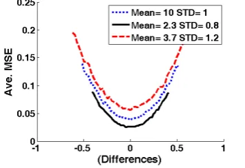
[image:3.595.306.547.224.376.2]

and take 50 pseudo means distributed uniformly over the interval as the candidates of population mean. Fig. 3 displays the average MSEs of QMLE versus

(

μ_ps−μ . It can be clearly found from the figure that, for all the three test cases using different normal distributions, the average MSEs of QMLE are characterized as convergence curves to become smaller as the absolute value of the difference between μ_ps and μ decreases.

Fig. 3: Average MSE of QMLE versus difference=

(

μ_ps−μ

)

for three normal distributions. Note that ξ_1:n is calculated using true standard deviation σ .

B. Asymptotic efficient near the minimal average of MSEs Fig. 3 shows that the three average MSE curves are convex functions of

(

μps−μ

)

with their minima located at the zero

of

(

μ_ps−μ

)

. Basing on the observation, we therefore suggest letting the selection criterion of the pseudo mean,

ps

μ , correspond to the minimal average MSE, and expect that the resulting QMLE has much higher efficiency than the sample mean.

C. Minimax structure for the objective function

Now, we add a punishment term to form a new objective function and find the optimal pseudo mean estimate by

(

* 2 * 2

)

1

: 2 1

: : : 2

1

1:

* 2

1: 1 1

arg max ( , ) ( ) ( )

2 1

arg max ( log 2 log ) ( )

2 2

( )

2 1

{(( ) ) 2

ps

ps

ps n

n

i p n

i n

i p n p n ps p n ps

i s s

n ps

n

s

QMLE

x x

n _n

x x x _n x

x x

μ

μ

σ μ μ μ μ μ

π σ

σ

μ μ

σ σ σ

μ

σ μ

σ

=

=

⎧ _{− − + −} ⎫

⎨ ⎬

⎩ ⎭

− ⎧

= ⎨ − − −

⎩

− − −

− ⋅ −

−

− − ⋅ −

∑

∑

:

* 2

:

(( n n ps) ) }

n n n

s

x

x σ μ μ

σ

− ⎫

+ − ⋅ − ⎬

⎭

(9)

The minimax operation is thus constructed completely. The corresponding criterion of optimization is a combination of maximum QMLE and MMSE on QSQ.

Table 1 lists four possible conditions that we will encounter in setting the inspection area for searching the optimal μps . They specify the conditions whether the

population’s mean and population’s standard uncertainty are given or not. Basically, the inspection area is set as

[μ−2 /σ n,μ+2 /σ n]. If the combined (population’s) mean is unknown, the best searching interval for determining the candidates is also unknown. In this case, we use the sample mean to determine the searching interval. Similarly, if the combined (population’s) standard uncertainty, σ , is unknown, we use the samples’ standard uncertainty, σS, for

its substitution.

Table 1: Table of confusion for the conditions of combined mean and combined standard uncertainty

Combined Mean (CLT searching interval)

Known Unknown

Known A B

STU of combined

quantities Unknown C D

D. QMLE optimization on MMSE of only the two endpoints of range, (QSQ)

[image:3.595.79.257.592.714.2]

quantiles obey the properties of symmetric quantiles, the QMLE mean estimator may be efficient and robust with variance asymptotically approaching the Cramer-Rao lower bound [13]. It is worthy noting that since the QSQ usually occupies (covers) the most percent of variance, it is therefore popular to apply the double censoring scheme for the observations of small sample size, especially in the sport contest. We know that adopting such a strategy can avoid the large variation occurring in the mean estimation. Based on above discussions, we apply the above QMLE+MMSE optimization search only on QSQ, and call it the Q2MMSE-CLT scheme.

We now examine the performance of Q2MMSE-CLT by simulations. Suppose that the combined quantity is composed of four independent random input quantities with two normal

distributions, and , and

two rectangular distributions, 2

1~ (0.1,1 )

x N 2

2 ~ (2.15,1.5

x N )

3 ~ [ 2 3 1.05, 2 3 1.05]

x rect− − − and

4 ~ [ 10 3 1.45,10 3 1.45]

x rect − + + . We perform 10,000

[image:4.595.83.254.405.531.2]

trials to test Q2MMSE-CLT for each of the four conditions listed in Table 1. The testing sample size ranges from 11 to 40 for each trial. Fig.4 and Fig. 5 display the experimental results. It can be found from these two figures that Q2MMSE-CLT significantly outperforms the sample mean for Conditions A and B, and is slightly better for Conditions C and D. In other words, Q2MMSE-CLT has much lower MSEs when the standard uncertainty is known.

Fig. 4: Average MSEs for Conditions A and C. y axis is normalized to 2_{( ) /}

c

u x n

Fig. 5: Average MSEs for Conditions B and D. y axis normalized to

2_{( ) /}

c

u x n

E. Test the robustness of Q2MMSE-CLT for different Uncertainty Ratio

Here we test Q2MMSE-CLT for two different values of UR. As demonstrated in Fig. 1, the R*N distribution is more flat in its central part as UR increases. It is a general issue to study whether Q2MMSE-CLT performs better for larger UR. We perform 10,000 trials for two cases of combined quantities composing of four different distributions. One has

, ,

2 (0.1,1 )

N _{N(0.2,1.5 )}2 _{rec[ 2 3 0.15, 2 3 0.15]− + + , and}

[ 10 3 0.1,10 3 0.1]

rec− − − . Its UR is equal to 3.7 evaluated according to Eq.(2). Another is the same as the first case except that rec[ 10 3 0.1,10 3 0.1]− − − is changed to

[ 28 3 0.1, 28 3 0.1]

rec− − − . The UR is accordingly

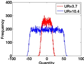
changed to 10.4. Fig. 6 displays the histograms of 50,000 outputs of combined quantities for the two cases. It shows the property of quasi-normal distribution for the output of combined quantities. To compare the two cases of Q2MMSE-CLT, a robustness function of gain relative to sample mean is defined as

2

( 2 _ )

1

( )

( ) ( : c )

Average MSEs of Q MMSE CLT G

Average MSEs of sample mean u x

unit n

= −

[image:4.595.356.499.430.539.2]

(10)

[image:4.595.359.502.567.677.2]

Fig. 7 displays the experimental results. It can be found from the figure that Q2MMSE-CLT outperforms sample mean for both cases of UR=3.7 and UR=10.4. Moreover, the performance is better for larger UR.

Fig. 6: Histogram of 50,000 combined quantities for different URs. x-axis is the output of combined quantities and y-axis is the frequency count

[image:4.595.84.255.577.711.2]

Condition D. As was noted previously, the testing data of combined quantities are formed in the same manner and we execute 1,000 trials with 15 observations in each trial. We select 60 candidates of population mean and arrange them symmetric to the sample mean within the interval of

[ 2− σ_s/ n x+ , 2σ_s/ n x+ ]. Then we evaluate the QMLE via the Q2MMSE-CLT scheme. In our maneuver, we first plot the convex curves according to the three different clusters of Z score (quantile of the signal transformed to standard normal pdf) of sample mean: Z< −2 ,

, and 0.5 Z 0.5

− ≤ ≤ Z>2. We then define the cluster as good sample mean and the other two clusters,

0.5 Z 0.5

− ≤ ≤

2

Z< − and Z>2, as the bad sample means. Fig. 8 is the convex sets conditioned on the good sample mean. Here, the dot line is the convex set for the original signal of combined quantities and the green solid line represents the convex set due to enlarging standard uncertainty (ESU) to 4 times of the original signal with the same reference candidates of population mean. We see from the figure that both the original and ESU signals take the Q2MMSE-CLT convergence near the symmetric location, the 30-th candidate in good sample mean, so that the good sample mean will guarantee the convergence to population mean on heavy observations.

Fig. 8: Good sample mean tested with the convex sets, normalized by , sample size is 15, 4 combined quantities

2_{( ) /}

c

[image:5.595.327.534.146.278.2]

u x n

Fig. 9 and Fig. 10 are, respectively, the results for the two cases of biased Z score less than -2 and greater than 2 when applying the Q2MMSE-CLT and enlarging standard uncertainty Q2MMSE-CLT (ESQ2MMSE-CLT). We plot the details shown as the double y-axes representation in which the dash line represents the original signal evaluated by Q2MMSE-CLT and the solid line represents the signal evaluated by ESQ2MMSE-CLT with 4 times of combined standard uncertainty. An important fact is found from the two figures that the original signal will be affected by the sample mean if it only takes the Q2MMSE-CLT operations. The resulting MSE curves converge to the near symmetric location which is the sample mean and we know it is the bad sample mean. We also found from these two figures that, as we apply the ESQ2MMSE-CLT algorithm with 4 times of combined standard uncertainty, the MSE curves converge to locations deviated away from the bad sample mean and toward the directions of population mean. Why does it act as the action? The reason is that the ESQ2MMSET-CLT enlarges the combined standard uncertainty to 4 times of the

[image:5.595.325.537.319.454.2]

original signal. Thus the Z score of the general maximum bias sample mean will be reduced to 25% of that of the original signal. It means that the Z score of bias is constrained to 0.5− ≤ ≤Z 0.5. The fact has been demonstrated in the green solid line of Fig. 8, that it will guarantee the convergence to the good sample mean, also the population mean.

[image:5.595.77.250.367.500.2]

Fig. 9: Left biased of bad sample mean tested with the convex sets, double y-axes, normalized by u x n_c2( ) / , sample size is 15, 4 combined quantities

Fig. 10: Right biased of bad sample mean tested with the convex sets, double y-axes, normalized by u x n_c2( ) / , sample size is 15, 4 combined quantities Fig. 11 displays the refined results of ESQ2MMSE-CLT for sample size from 11~40. We find from the figure that ESQ2MMSE-CLT significantly outperforms the sample mean by 40% MSE reduction. So it is a promising mean estimator.

[image:5.595.337.506.575.706.2]

V. CONCLUSIONS

In this paper, the issue of applying quantile-based maximum likelihood estimation (QMLE) to mean value estimation of normal distribution in sparse data condition was addressed. It proposed to incorporate order statistics into QMLE to take the maximum coverage as quantiles so as to conform to the requirement of symmetric quantiles. Simulation results have confirmed that the new Q2MMSE-CLT performs very well to outperform the conventional sample mean estimator. We showed that the Q2MMSE-CLT earns the gain with the greatest utilities when the combined mean is known and obtains the least benefits if we take the sample mean to substitute for the combined mean. In spite of that fact, ESQ2MMSE-CLT can compensate this shortcoming. The robustness of ESQ2MMSE-CLT to its usage of sample mean makes it a promising mean estimator for practical applications.

One thing must be paid attention that Q2MMSE-CLT is free to the standard uncertainty of population so that the combined standard uncertainty of combined quantities can be ignored and replaced with the samples’ standard uncertainty in the estimation process.

APPENDIX:

The Quantile-based mean estimator:

By substituting μ=x_{p n:} −σξ_{p n:} , for 1 p= or n , into

( , )

QMLE μ σ defined in Eq.(5), we obtain

: 2 1

: 2

: :

1

1

( , ) ( log 2 log ) ( )

2 2

2

n

i p n

i n

i p n

p n p n

i

x x n

QMLE n

x x n

μ σ π σ

σ

ξ ξ

σ

=

=

−

= − − −

−

− ⋅ −

∑

∑

(11)

Taking the partial derivative of Eq.(11) with respect to σ

and setting it to zero, we obtain

2 2

: : :

1 1

( ) ( )

n n

p n i p n i p n

i i

nσ ξ x x σ x x

= =

−

∑

− −

∑

− =0 (12)

Solve Eq.(12) to obtain an estimate of the standard deviation of population:

( )

2

* 4

2

B B nC

n

σ σ

σ = ± + σ

(13) where

: :

1

( )

n

p n i p n

i

Bσ ξ x x

=

=

∑

− 2

: 1

( )

n

i p n

i

x σ

=

=

∑

−

, C x , and _σ* _>0.

REFERENCES

[1] JCGM, “Evaluation of measurement data —supplement 1 to the guide to the expression of uncertainty in measurement— propagation of distributions using a Monte Carlo method,” Joint Committee for Guides in Metrology, final draft, 2006.

[2] P. Fotowicz, “An analytical method for calculating a coverage interval,” Metrologia, vol. 43, pp.42-45, 2006

[3] P. Fotowicz, “A method approximation of the coverage factor in calibration,” Measurement, vol. 35, pp.251-256, 2004.

[4] B. A. Bowen, “An alternate proof of the central limit theorem for sums of independent processes,” Proceedings of the IEEE, vol. 54, iss. 6, pp. 878-879, 1966.

[5] D. T. Searls, “The utilization of a known coefficient of variation in the estimation procedure,” Journal of American Statistical Association, vol. 59, pp. 1225-1226, 1964.

[6] L. J. Gleser and J. D. Healy, “Estimating the mean of a normal distribution with known coefficient of variation,” Journal of American Statistical Association, vol. 71, pp, 977-981, 1976

[7] Ashok Sahai, M. Raghunadh and Hydar Ali, “Efficient estimation of normal population mean,” Journal of Applied Science, vol. 6, iss. 9, pp. 1966-1968, 2006.

[8] ISO, “Guide to the expression of uncertainty in measurement (GUM)—Supplement1: Numerical methods for the propagation of distributions,” International Organization for Standardization, 2004, p.12.

[9] R. Koenker and G.J. Bassett, “Regression quantiles,” Econometrica, vol. 46, pp. 33–50, 1978.

[10] W. G. Gilchrist, “Statistical modeling with quantile function,” London: Chapman and Hall/CRC, 2002

[11] G. GIORGI and C. NARDUZZI “Uncertainty of quantile estimates in the measurement of self-similar processes,” In: Workshop on Advanced Methods for Uncertainty Estimation Measurements, AMUEM 2008, pp.78-83.

[12] A. Heathcote, S. Brown, and D. J. K. Mewhort, “Quantile maximum likelihood estimation of response time distribution,” Psychonomic Bulletin and Review, 2002.

[13] L.-A. Chen and Y.-C. Chiang, “Symmetric type quantile and trimmed means for location and linear regression model,” Journal of Nonparametric Statistics, vol. 7, pp. 171–185, 1996.

[14] W.-H. Lo and S.-H. Chen, “The analytical estimator for sparse data,” International Association of Engineers (IAENG) Journal of Applied Mathematics, vol. 39, iss. 1, 2009, pp. 71-81.

[15] W.-H Lo and S.-H. Chen, “Robust estimation for sparse data,” The 19-th international conference on pattern recognition, 2008, pp.1-5. [16] Peter J. Huber, “Robustr statistics: a review,” Ann. Math. Stat. vol. 43,