A Prior Error Estimate for Linear Finite Element
Approximation to Interface Optimal Control
Problems
Hongbo Guan, Chaoyang Hao, Yapeng Hong, and Pei Yin
Abstract—This paper considers a linear finite element method for the constrained optimal control problems (OCPs) governed by elliptic interface equations. The state and adjoint state are approximated by the conformingP1elements, while the control
is approximated with the orthogonal projection of the adjoint state. Optimal order error estimates are proved in both L2 -norm and broken energy -norm. Lastly, some numerical results are presented to confirm the theoretical analysis.
Index Terms—finite element method, interface OCPs, optimal order error estimates.
I. INTRODUCTION
O
Ptimal control problems (OCPs) governed partial dif-ferential equations are playing an increasingly crucial role in a lot of engineering applications, such as chemical processes, fluid dynamics, medicine, economics, and so on [3], [24]. Much attention has been paid to the numerical solution of these problems since their analytical solutions do not always exist. In the recent decades, finite element methods (FEM) have been developed to be one of the most popular and efficient methods not only for partial differential equations [26], but also for many scientific com-puting fields, i.e., the magnetic resonance elastography [18], mechanism analysis [19], predicting the blasting effect [27], etc. Recently, FEMs have been intensively investigated for OCPs governed by partial differential equations. A priori error estimate was firstly proposed in [6] for the OCPs and obtained the error estimates in L2-norm. [14] derivedthe error estimates of FEM for an elliptic OCPs with a small parameter. Mixed FEM for OCPs governed by elliptic equations and Stokes equations was presented in [4] and [15]. On the other hand, some a posteriori error estimates of conforming FEMs for the OCPs were reported in [12], [13], [21] and the references cited therein. In addition, some
Manuscript received May 24, 2019; revised August 08, 2019. This work was supported by the National Natural Science Foundation of China (Nos. 11501527 and 71601119), 2015 PhD Start-up Project of ZZULI (2015BSJJ070), Excellent Young Scholars Foundation of ZZULI (Grant no. 2016XGGJS008), Graduate Student Innovative Foundation of ZZULI (Grant no. 2018018), Humanities and Social Science Foundation of Ministry of Education (16YJCZH138), “Chenguang Program” supported by Shanghai Education Development Foundation and Shanghai Municipal Education Commission(16CG53), 2016 “Pandeng” Project of Humanities and Social Science Foundation of USST(SK18PB02), The financial support is gratefully acknowledged.
Hongbo Guan and Yapeng Hong are with College of Mathematics and Information Science, Zhengzhou University of Light Industry, Zhengzhou 450002, China.
Chaoyang Hao is with Department of Mathematical Sciences, Tongji University, Shanghai 200092, China.
Corresponding author. Pei Yin is with Business School, University of Shanghai for Science and Technology, Shanghai 200093, China. E-mail: [email protected]
discussions on nonconforming FEMs for OCPs can be found from [7], [8], [10], [11].
We consider the following interface OCPs: find(y, u)∈
Y ×U, such that
min u∈Uad⊂U
J(y, u) =1
2ky−ydk
2 0,Ω+
α
2kuk
2
0,Ω (1)
subject to
−∇ ·(β∇y) =u, inΩ, y= 0, on∂Ω,
[y]Γ = 0,[β∂y∂n]Γ= 0,
(2)
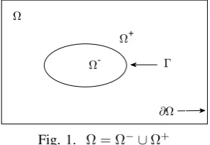
where α is a positive constant parameter, Ω is a convex polygon in R2. Let Ω− ⊂ Ω be an open domain with
a C2 curve boundary Γ ⊂ Ω, and let Ω+ = Ω \ Ω−
(see Fig.1). Throughout this paper, we use the standard
[image:1.595.353.501.406.508.2]-+
Fig. 1. Ω = Ω−∪Ω+
Sobolev spaces and norms (see [2]), and further denote Y =H1
0(Ω)∩H2(Ω−)∩H2(Ω+), and U = H1(Ω). The
target state yd∈C0(Ω) is a given function. The admissible
control setUad is defined as
Uad={v∈U :a(x)≤v≤b(x), a.e. inΩ}, (3)
in whicha(x), b(x)∈L∞(Ω), anda(x)< b(x).
In (2), we denote by[v]Γthe jump ofvacross the interface Γ and n the unit outward normal to Γ, respectively. The coefficientβis a positive piecewise constant function defined by
β(x) =βs, x∈Ωs, (4) wheres=−or +.
The interface OCP (1)-(2) has remarkable application backgrounds, such as the optimization or optimal control of a process in a domain which is composed of several materials separated by interfaces. Coefficients in partial differential equations may have a jump across the interface among different materials. There are mainly two approaches for numerically solving interface OCPs by using FEM. The first one is to utilize conventional FEMs or its variations
IAENG International Journal of Applied Mathematics, 50:1, IJAM_50_1_14
defined on a body-fitted mesh for the domain that contains a interface [1]. Another approach that has drawn more attention recently is the so-called immersed FEM [16], [17], [25]. This method constructs a finite element space that allows piecewise continuous basis functions on each element in order to approximate the interface jump conditions.
In this paper, we present aP1-conforming triangular
body-fitted FEM approximation to the elliptic interface OCP (1)-(2), which could also be extended to parabolic and hyperbolic OCPs. This method was studied in [5] for solving interface problems and obtained the suboptimal order error estimates inH1andL2norms when the interface is ofC2smooth. The
authors of this paper also pointed out that the error estimate inH1 norm can be optimal if the exact solution belongs to
W1,∞ near the interface (cf. Remark 2.4 in [5]). Later on,
[23] provided the detailed proof of the above statement, and [9] extended this method to P1-nonconforming element.
The remainder of this paper is organized as follows: in Section II, we present the discrete formulations and some useful lemmas. Then, in Section III, we derive the optimal order error estimates for both the state variable and the control variable. In the last section, some numerical results are given to verify the validity of the proposed method.
II. THE DISCRETE FORMULATION AND SOME LEMMAS We know from [20] that (1)-(2) has a unique solution
(y, u) if and only if there is an adjoint state p ∈ Y, such that (y, p, u)satisfies the following optimality conditions:
a(y, v) = (u, v), ∀v∈Y,
a(p, v) = (y−yd, v), ∀v∈Y,
(αu+p, v−u)≥0, ∀v∈Uad,
(5)
wherea(y, v) = Z
Ω
β∇y∇vdx;(u, v) = Z
Ω
uvdx;p∈Y is the adjoint state variables. Specifically, the second equation of (5) is the weak form of
−∇ ·(β∇p) =y−yd, inΩ,
p= 0, on∂Ω,
[p]Γ= 0, [β∂n∂p]Γ= 0,
(6)
wherepalso satisfies the jump condition as same asyfor it in (1).
In addition, with the admissible control set (3), we can get the explicit representation of the optimal control uthrough the adjoint statep,
u(x) = PUad
−1
αp(x)
= min
b(x),max
a(x),−1
αp(x)
, (7)
in which PUad denotes the orthogonal projection operator
ontoUad.
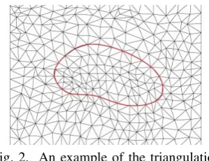
Next, we introduce a quasi-uniform triangulation Th =
{K} of the domainΩas in [5], [9]. We denote the diameter of K byhK, and leth= max
K∈Th
hK.
To decompose the interface Γ, we first approximate the domain Ω− by a regionΩ−h with a polygonal boundary Γh
whose vertices all lie on the interfaceΓ. LetΩ+h = Ω−Ω−h. Then, we require eachK∈Th to satisfy the following two
conditions (see Fig. 2):
(i)K is either inΩ−h or in Ω+h;
(ii) For any edge F, F has either vertices or the whole edge lying onΓ ifF∩Γ6=∅.
We callKan interface element if it intersectsΓand denote the set of interface elements by Th∗. For eachK ∈Th∗, let K−=K∩Ω−andK+=K∩Ω+. BecauseΓisC2smooth, it implies either meas(K−) ≤ ch3
K or meas(K
+) ≤ ch3 K.
Throughout this paper, we will useK˜ to denote one of the two subregions K− and K+ which satisfies meas(Ks) ≤
ch3
K. Here and later, c denotes a generic positive constant
[image:2.595.350.500.213.328.2]independent of h but may take different values at different occasions.
Fig. 2. An example of the triangulation
On triangulationTh we construct the piecewiseP1 linear
conforming finite element spaceVhsuch thatVh⊂H01(Ω)∩
C(Ω), and defineΠh : H1(Ω)→ Vh to be the associated
interpolation operator.
The corresponding discrete form of (1)-(2) reads as: find
(yh, uh)∈Vh×Uad,such that min
uh∈Uad
Jh(yh, uh) = 1
2kyh−ydk
2 0,Ω+
α
2kuhk
2
0,Ω, (8)
subject to
ah(yh, vh) = (uh, vh), ∀vh∈Vh, (9)
where ah(yh, vh) = X
K∈Th Z
K
βh∇yh∇vhdx, βh = βs if
K⊂Ωs h.
Similar to (5), we seek a unique solution (yh, ph, uh)
satisfying the following discrete optimality conditions:
ah(yh, vh) = (uh, vh), ∀vh∈Vh,
ah(ph, vh) = (yh−yd, vh), ∀vh∈Vh,
(αuh+ph, vh−uh)≥0, ∀vh∈Uad,
(10)
where the optimal controluhwill be solved from the adjoint
stateph,
uh = PUad
−1
αph
= min
b(x),max
a(x),−1
αph
.
(11)
The following lemma has been presented in [5], which plays an important role in our theoretical analysis.
Lemma 2.1Letf ∈L2(Ω), andΩ
0∈Ωbe a neighborhood
of the interfaceΓ. Suppose thatϕ∈Y ∩W1,∞(Ω−∩Ω 0)∩
W1,∞(Ω+∩Ω
0)andϕh∈Vh are solutions of
a(ϕ, v) = (f, v), ∀v∈H01(Ω), (12)
and
ah(ϕh, vh) = (f, vh), ∀vh∈Vh, (13)
IAENG International Journal of Applied Mathematics, 50:1, IJAM_50_1_14
respectively. Then, there hold the following error estimate results:
|a(ϕ, vh)−ah(ϕh, vh)| ≤chkϕkY,Ω (14)
and
kϕ−Πhϕk0,Ω+h|ϕ−Πhϕ|1,Ω ≤ch2kϕkY,Ω,
kϕ−ϕhk0,Ω+h|ϕ−ϕh|1,Ω ≤ch2kϕkY,Ω,
(15)
wherekϕkY,Ω:=
q
kϕk2
1,Ω+|ϕ|22,Ω++|ϕ|22,Ω−. III. OPTIMAL ORDER ERROR ESTIMATES
This section proceeds in two steps. First, we present optimal order error estimates and detailed proof of the state y and adjoint statepinL2-norm. Second, the optimal order error estimate of the stateyand adjoint statepin the broken-energy norm will be proved in Theorem 3.2.
Theorem 3.1.Let(u, y, p)∈Uad×Y×Y and(uh, yh, ph)∈
Uad×Vh×Vh be the solutions of (1) and (8), respectively.
Then, there holds the following error estimate:
ku−uhk0,Ω+ky−yhk0,Ω+kp−phk0,Ω≤ch2. (16)
Proof. Replacingvandvhwithuhanduin the inequalities
of (5) and (10) yields
(αu+p, u−uh)≤0, (17)
and
(αuh+ph, uh−u)≤0. (18)
Then, it follows from summing up the above two inequalities and Lemma 2.1 that
αku−uhk20,Ω
≤(uh−u, p−ph)
= (uh−u, p−ph(y)) + (uh−u, ph(y)−ph)
= (uh−u, p−ph(y)) +ah(yh−yh(u), ph(y)−ph).
(19) The first term on the right hand side of the above inequality can be estimated as follows:
(uh−u, p−ph(y))
≤α
2kuh−uk 2 0,Ω+
1
2αkp−ph(y)k 2 0,Ω.
(20)
Then, we are going to estimate the second term on the right hand side of (19). Actually, we have
ah(yh−yh(u), ph(y)−ph)
=ah(yh−yh(u), ph(y))−ah(yh−yh(u), ph)
= (yh−yh(u), y−yd)−(yh−yh(u), yh−yd)
= (yh−yh(u), y−yh)
= (yh−y, y−yh) + (y−yh(u), y−yh)
≤ 1
2ky−yh(u)k 2 0,Ω−
1
2ky−yhk 2 0,Ω,
(21)
whereyh(u)∈Vh andph(y)∈Vh are the solutions of
ah(yh(u), vh) = (u, vh), ∀vh∈Vh, (22)
and
ah(ph(y), vh) = (y−yd, vh), ∀vh∈Vh, (23)
respectively.
Summarizing the above two inequalities and substituting it into (19) lead to
αku−uhk20,Ω+ky−yhk20,Ω
≤ kp−ph(y)k20,Ω+αky−yh(u)k20,Ω.
(24)
Noticing thatph(y)andyh(u)are standard finite element
approximations of p and y. As a consequence, by Lemma 2.1, we have
kp−ph(y)k0,Ω≤ch2kpkY,Ω (25)
and
ky−yh(u)k0,Ω≤ch2kykY,Ω. (26)
Combining (24), (25)and (26) gives that
ku−uhk0,Ω+ky−yhk0,Ω≤ch2. (27)
In the following, we consider the estimate ofkp−phk0,Ω.By
the definition of bilinear form ah(·,·)and (10), there exists
a positive numberc0 such that
c0kph(y)−phk20,Ω ≤ah(ph(y)−ph, ph(y)−ph)
= (ph(y)−ph, y−yh)
≤ckph(y)−phk0,Ωky−yhk0
≤ch2kph(y)−phk0,Ω,
(28) which implies that
kph(y)−phk0,Ω≤ch2. (29)
Combining (25) and (29) yields
kp−phk0,Ω≤ch2. (30)
The proof is completed.
Now we are ready to derive the optimal order error estimates for the state y and adjoint state p in the broken energy norm.
Theorem 3.2. Under the assumption of Theorem 3.1, there hold the following optimal order error estimates for state y and adjoint statep:
|y−yh|1,Ω≤ch (31)
and
|p−ph|1,Ω≤ch, (32)
respectively.
Proof. First of all, letβ∗ = min{β−, β+}. We have
β∗|y−yh|21,Ω≤ah(y−yh, y−yh)
=ah(y−yh, y−Πhy) +ah(y−yh,Πhy−yh).
(33) The bound of the first term of (33) can be found directly from Schwarz inequality and the standard approximation theory, i.e.,
ah(y−yh, y−Πhy) ≤ c|y−yh|1,Ω|y−Πhy|1,Ω
≤ β∗
4|y−yh| 2
1,Ω+c|y−Πhy|21,Ω
≤ ch2+β∗
4|y−yh| 2 1,Ω.
(34)
IAENG International Journal of Applied Mathematics, 50:1, IJAM_50_1_14
The estimation of the second term of (33) follows from the results of Lemma 2.1, Theorem 3.1, and the standard approximation theory
ah(y−yh,Πhy−yh)
≤(u−uh,Πhy−yh) +chkykY,Ω|Πhy−yh|1,Ω
≤ ku−uhk0,ΩkΠhy−yhk0,Ω+chkykY,Ω|Πhy−yh|1,Ω
≤c h4+h2kyk2
Y,Ω+kΠhy−yk21,Ω
+β∗
4|y−yh| 2 1,Ω
≤ch2+β∗
4|y−yh| 2 1,Ω.
(35) Summarize the above two inequalities into (33) yields (31). Similarly, for the adjoint state p, using again Lemma 2.1 and Theorem 3.1, we have
β∗|p−ph|21,Ω
≤ah(p−ph, p−ph)
=ah(p−ph, p−Πhp) +ah(p−ph,Πhp−ph)
≤ah(p−ph, p−Πhp) + (y−yh,Πhp−ph)
+ch|Πhp−ph|1,Ω
≤c|p−ph|1,Ω|p−Πhp|1,Ω+ky−yhk0,Ω|Πhp−ph|1,Ω
+ch|Πhp−ph|1,Ω
≤ch|p−ph|1,Ω+ch(|Πhp−p|1,Ω+|p−ph|1,Ω)
≤ch|p−ph|1,Ω+ch2kpkY,Ω
≤ch2+β∗
2|p−ph| 2 1,Ω,
(36) which gives (32). The proof is thus completed.
IV. NUMERICAL EXPERIMENT
This section will provide some numerical results for the elliptic interface control problem to verify the correctness of the theorems given in the previous section.
In this example we choose α = 1 and the computation domain as Ω=[−1,1]×[−1,1], the interface Γ is a circle centered at the origin with radius being r0 = 0.5. Ω− =
{(x1, x2)|x21+x22≤0.5},Ω+=Ω−Ω−.
The admissible control setUad is given as
Uad={v∈U :−1≤v≤1, a.e. inΩ}. (37)
We take the optimal state and adjoint state as
y=
u−= (x21+x 2 2)
3/2
β− , inΩ−, u+= (x21+x22)3/2
β− + (β1− −β1+)r
3
0, inΩ+,
(38)
and
p= (
p−= 5(x2
1+x22−r20)(1−x1)(x1+1)(x2−1)(x2+1)
β− , inΩ−,
p+= 5(x21+x22−r02)(1−x1)(x1+1)(x2−1)(x2+1)
β+ , inΩ
+,
(39) respectively.
The optimal control could be expressed as
u(x) = PUad{−p(x)}
= min{1,max (−1,−p(x))}. (40)
Then the functionsf andyd can be determined the above
functions accordingly.
In this experiment, we fixβ−=−1, and considerβ+= 5
andβ+= 50as two cases. We first approximate the circleΓ
by a polygon, and then give triangular subdivision to these
two domains separately. A uniform triangle grid mesh is thus completed. The error estimates and convergence orders of the control, state and adjoint state are shown in the following Tables 1-4 forβ+ = 5 andβ+ = 50, and the convergence
rates are reported in Figures 3-6, where N denotes the number of the elements, ”order” represents the convergence order which is evaluated by
Order= 1
log(N2/N1)1/2
logku−uN1ki,Ω
ku−uN2ki,Ω
, (41)
[image:4.595.325.527.214.326.2]here,ku−uNki is a special norm for i= 0,1.
Table 1 The errors and convergence orders inL2-norm withβ+= 5 N ku−uhk0,Ω ky−yhk0,Ω kp−phk0,Ω
14 0.318638863 1.189625451 0.097867163
order / / /
72 0.065900590 0.248701791 0.021369779
order 1.92465 1.91149 1.85836
322 0.013276842 0.061789328 0.005924887
order 2.13918 1.85932 1.71284
1458 0.002700346 0.012417775 0.001352403
order 2.10908 2.12492 1.95631
2982 0.001287701 0.005823426 0.000638279
[image:4.595.325.528.373.479.2]order 2.06986 2.11659 2.09876
Table 2 The errors and convergence orders in energy norm withβ+= 5
N |y−yh|1,Ω |p−ph|1,Ω
14 0.164654461 0.003396546
order / /
72 0.073176671 0.001588027
order 0.99043 0.92851
322 0.032943245 0.000887296
order 1.06562 0.77719
1458 0.018774017 0.000390204
order 0.74465 1.08790
2982 0.012140199 0.000271377
order 1.21854 1.01508
10-3 10-2 10-1 100
h
10-4 10-3 10-2 10-1 100 101
The convergence order of L
2-norm with
-+=5
u y p
Fig. 3. Convergence rates ofL2 norm with β+= 5
IAENG International Journal of Applied Mathematics, 50:1, IJAM_50_1_14
[image:4.595.46.295.527.722.2]10-3 10-2 10-1 100
h
10-4 10-3 10-2 10-1 100
The convergence order of energy norm with
-+=5 y
p
[image:5.595.56.282.62.240.2]Fig. 4. Convergence rates of energy norm withβ+= 5
Table 3 The errors and convergence orders inL2-norm withβ+= 50
N ku−uhk0,Ω ky−yhk0,Ω kp−phk0,Ω
14 0.678309069 3.631292383 0.171599428
order / / /
72 0.146790976 0.81557836 0.039212493
order 1.86930 1.82394 1.80283
322 0.039629437 0.214722199 0.010928453
order 1.74838 1.78192 1.70591
1458 0.00858952 0.049549885 0.003454323
order 2.02484 1.94186 1.52522
2982 0.004611587 0.023641828 0.001747589
order 1.73849 2.06830 1.90458
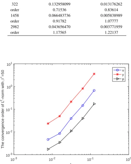
Table 4 The errors and convergence orders in energy norm withβ+= 50
N |y−yh|1,Ω |p−ph|1,Ω
14 0.537165421 0.062955460
order / /
72 0.227192916 0.024646492
order 1.05093 1.14532
322 0.132958099 0.013176262
order 0.71536 0.83614
1458 0.066483736 0.005838989
order 0.91782 1.07777
2982 0.043656470 0.003771959
order 1.17565 1.22137
10-3 10-2 10-1 100
h
10-3 10-2 10-1 100 101
The convergence order of L
2-norm with
-+=50
[image:5.595.311.537.62.239.2]u y p
Fig. 5. Convergence rates of L2 norm with β+= 50
10-3 10-2 10-1 100
h
10-3 10-2 10-1 100
The convergence order of energy norm with
-+=50
[image:5.595.68.271.296.408.2]y p
Fig. 6. Convergence rates of energy norm withβ+= 50
We can see that this linear body-fitted method could achieve a optimal order convergence, which almost coincides with our theoretical analysis.
Remark 1.It is worth mentioning that the fact (∇vh)|K =
constant for all vh ∈ Vh is crucial in the error
analy-sis, which implies that the idea in the error analysis can be apply to P1−nonconforming triangular element [9] and
P1−rectangular element [22]. However, this approach could
not be generalized to higher order elements.
Remark 2. With properly handling the time variable, the results obtained in this paper could be extended to some time-dependent OCPs, such as parabolic and hyperbolic interface control problems.
REFERENCES
[1] I. Babuˆska, “The finite element method for elliptic equations with discontinuous coefficients,”Computing, vol. 5, no. 3, pp. 207-213, 1970. [2] S. C. Brenner and L. R. Scott, The Mathematical Theory of Finite
Element Methods, Berlin: Springer-Verlag, 1994.
[3] G. G. Chen, X. T. Yi, Z. Z. Zhang and S. Y. Qiu, “Solving optimal power flow using cuckoo search algorithm with feedback control and local search mechanism,”IAENG International Journal of Computer Science, vol. 46, no. 2, pp. 321-331, 2019.
[4] Y. P. Chen, “Superconvergence of mixed finite element methods for optimal control problems,”Mathematics of Computation, vol. 77, no. 263, pp. 1269-1291, 2008.
[5] Z. M. Chen and J. Zou,“Finite element methods and their convergence for elliptic and parabolic interface problems,”Numerische Mathematik, vol. 79, no. 2, pp. 175–202, 1998.
[6] F. S. Falk,“Approximation of a class of optimal control problems with order of convergence estimates,”Journal of Mathematical Analysis and Applications, vol. 44, no. 1, pp. 28-47, 1973.
[7] H. B. Guan and D. Y. Shi,“A high accuracy NFEM for constrained optimal control problems governed by elliptic equations,” Applied Mathematics and Computation, vol. 245, no. 19, pp. 382-390, 2014. [8] H. B. Guan and D. Y. Shi,“A nonconforming finite element method for
constrained optimal control problems governed by parabolic equations,” Taiwanese Journal of Mathematics, vol. 21, no. 5, pp. 1193-1211, 2017. [9] H. B. Guan and D. Y. Shi,“P1-nonconforming triangular FEM for elliptic and parabolic interface problems,” Applied Mathematics and Mechanics, vol. 36, no. 9, pp. 1197-1212, 2015.
[10] H. B. Guan, D. Y. Shi and X. F. Guan,“High accuracy analysis of nonconforming MFEM for constrained optimal control problems governed by Stokes equations,”Applied Mathematics Letters, vol. 53, no. 3, pp. 17-24, 2016.
[11] H. B. Guan, D. Y. Shi,“An efficient NFEM for optimal control problems governed by a bilinear state equation,”Computers and Math-ematics with Applications, vol. 77, no. 1, pp. 1821-1827, 2019. [12] W. Gong, W. B Liu, Z. Y. Tan and N. N. Yan,“A convergent adaptive
finite element method for elliptic Dirichlet boundary control problems,” IMA Journal of Numerical Analysis, vol. 22, pp. 1-31, 2018.
IAENG International Journal of Applied Mathematics, 50:1, IJAM_50_1_14
[image:5.595.56.278.480.757.2][13] W. Gong and N. N. Yan,“Adaptive finite element method for elliptic optimal control problems: convergence and optimality,” Numerische Mathematik, vol. 135, no. 4, pp. 1121-1170, 2017.
[14] W. Gong and N. N. Yan,“Robust error estimates for the finite element approximation of elliptic optimal control problems,”Journal of Com-putational and Applied Mathematics, vol. 236, pp. 1370-1381, 2011. [15] M. D. Gunzburger,“Analysis and finite element approximation of
optimal control problems for the stationary Navier-Stokes equations with distributed and neumann controls,”Mathematics of Computation, vol. 57, no. 195, pp. 123-151, 1991.
[16] X. M. He, T. Lin and Y. P. Lin,“Immersed finite element methods for elliptic interface problems with non-homogeneous jump conditions,” International Journal of Numerical Analysis and Modeling, vol. 8, no. 2, pp. 284-301, 2011.
[17] X. M. He, T. Lin and Y. P. Lin,“The convergence of the bilinear and linear immersed finite element solutions to interface problems,” Numerical Methods for Partial Differential Equations, vol. 28, no. 1, pp. 312-330, 2012.
[18] L. Hollis, E. Barnhill, N. Conlisk, L. E. J. Thomas-Seale, N. Roberts, P. Pankaj and P. R. Hoskins, “Finite element analysis to compare the accuracy of the direct and MDEV inversion algorithms in MR elastography,”IAENG International Journal of Computer Science, vol. 43, no.2, pp. 137-146, 2016.
[19] P. Ju, “Rock breaking mechanism analysis and structure design of the conical PDC cutter based on finite element method”Engineering Letters, vol. 27, no.1, pp. 75-80, 2019.
[20] J. L. Lions,Optimal Control of Systems Governed by Partial Differ-ential Equations, Berlin: Springer-Verlag, Berlin, 1971.
[21] W. B. Liu and N. N Yan,“A posteriori error estimates for control problems governed by Stokes equations,”SIAM Journal on Numerical Analysis, vol. 40, no. 5, pp. 1850-1869, 2002.
[22] D. Y. Shi, H. J. Yang,“Superconvergence analysis of a new low order nonconforming MFEM for time-fractional diffusion equation,”Applied Numeical Matematics, vol. 131, pp. 109-122, 2018.
[23] R. K. Sinha and B. Deka,“A priori error estimates in the finite element method for nonself-adjoint elliptic and parabolic interface problems,” Calcolo, vol. 43, no. 4, pp. 253-278, 2006.
[24] Z. D. Tian, S.J. Li, Y. H. Wang and B. Gu, “Priority scheduling of networked control system based on fuzzy controller with self-tuning scale factor,”IAENG International Journal of Computer Science, vol. 44, no. 3, pp. 308-315, 2017.
[25] Q. Zhang, K. Ito, Z. L. Li and Z. Y. Zhang,“Immersed finite elements for optimal control problems of elliptic PDEs with interfaces,”Journal of Computational Physics, vol. 298, pp. 305-319, 2015.
[26] M. C. Zhao, H. B. Guan and P. Y. Yin,“A stable mixed finite element scheme for the second order elliptic problems,”IAENG International Journal of Applied Mathematics, vol. 46, no. 4, pp. 545-549, 2016. [27] J. M. Zhou, X. .G. Wang, H. M. An, M. S. Zhao, M. Gong,“The
analysis of blasting seismic wave passing through cavity based on SPH-FEM coupling method,”Engineering Letters, vol. 27, no. 1, pp. 114-119, 2019.