On Young Functionals Related to Certain Class of
Rapidly Oscillating Sequences
Andrzej Z. Grzybowski,
Member, IAENG,
Piotr Puchała
Abstract—The paper is devoted to theory of classical Young measures and associated with them Young functionals i.e. certain mappings that assign to any Carathodory function an integral with respect to related Young measure. The main result provides us with probabilistic characterization of such mea-sures in the case where associated sequence of fast oscillating functions has uniform representation - a notion introduced in this paper. In many interesting cases this new characterization enables one to find an explicit formulae for the density functions of the Young measures and thus also to compute effectively the values of corresponding Young functionals. In other cases, where the explicit formulae for the densities cannot be received, the main result makes it possible to take advantage of Monte Carlo methods to evaluate the Young functional’s values.
Index Terms—Young measures, Young functionals, fast-oscillating sequences, periodic functions, Monte Carlo.
I. INTRODUCTION
T
HEre are many physical phenomena that can be de-scribed and explained by analysis of the suitable func-tionals corresponding to the respective physical quantities. The natural way of analysis of such functionals can be performed with the use of variational methods, among of which the minimization methods are one of the most pow-erful. Their usage can be justified as a conclusion from the variational laws of nature such as, say, the least action principle. Therefore there is no surprise that variational methods have been proved useful in engineering. One may look at [1], [2], [3], [5], [9], [10], or at books [11], [13] (and the references cited there) to mention just a few examples from vast literature on this subject.In general, we minimize the energy functional J of the form
J(u) = Z
Ω
H x, u(x),∇u(x)
dx,
whereRd⊃Ωis a bounded Lipschitz domain;u: Ω→K⊂
Rl is a function from a suitable Sobolev space V (withK
being a compact set); andH: Ω×Rd×Rld→R∪{+∞}is a function satisfying certain growth and regularity conditions. In the nonlinear elasticity theory we haved=l= 3,Ωis the considered elastic body, uis the displacement of Ω,H
is density of the internal energy (it usually depends on some physical constants).
The functional J is bounded below ’by nature’ so there exists a minimizing sequence for J, that is a sequence
{uk} ⊂V such that
lim
k→∞J(uk) = inf{J(v) :v∈V}.
Manuscript received June 6, 2017; revised June 15, 2017.
A.Z. Grzybowski and P. Puchała are with the Institue of Mathemat-ics, Faculty of Mechanical Engineering and Computer Science, Czesto-chowa University of Technology, CzestoCzesto-chowa, 42-201 Poland, e-mail: [email protected], [email protected]
However in general, for example when minimizing energy functionals corresponding to the multi-well potentials, the integrand does not satisfy convexity condition guaranteeing achieving by J its infimum. In that case elements of the minimizing sequence are the functions that oscillate rapidly around the weak (or weak∗) limit of that sequence. This situation is met in engineering for example when energy functionals of certain alloys are minimized. With the help of microscope one can observe what is by engineers called a ’microstructure’ – a structure somehow between the micro-and macroscoping scale.
The following example shows the crucial role of rapid oscillations in the arising of microstructure, [13]. Consider a function sequence {sinkx}, k ∈ N, defined on an
interval (0,π2). On one hand we have π 2
R
0
sin(kx)dx →
π 2
R
0
0dx, as k → ∞, while on the other π 2
R
0
sin2(kx)dx →
π
4 6=
π 2
R
0
02dx.
This in particular shows that even when the func-tion ϕ is continuous and a function sequence uk satysfies limR
uk(x)dx = R
u0(x)dx, the equality
limR
ϕ(uk(x))dx=R
ϕ(u0(x))dx does not have to be true
in general.
More generally we can say: the existence of the weak limit of a function sequence does not guarantee even the existence of the weak limit of the sequence whose elements are compositions of the elements of the aforementioned sequence with fixed (even continuous) function.
In the context of the variational methods a generalization of the above example is presented in [11], see also [7].
One of the ways of dealing with such problems is the L. C. Young’s idea: enlarging the space of admissible functions from Sobolev spaces to the space of parametrized measures
ν:={νx}x∈Ω,which are now calledYoung measures. Young
measures theory has a long history. It starts with the seminal work [15] where the main concept was introduced with the aim to provide extended solutions for some non-convex problems in variational calculus. After then Young developed his pioneering ideas in [16]. These ”generalized limits” of oscillating sequences where called by Young himself ”gener-alized curves” in the one dimensional case, and ”gener”gener-alized surfaces” in more general situation. Nowadays this concept has found applications in the solution of various non-convex optimization problems - that are at the core of many different contemporary engineering theories. They arise e.g. in optimal control, nonlinear evolution equation, variational calculus, micromagnetic phenomena in ferro-magnetic materials as well as in microstructures theory in continuum mechanics. It turns out that even the simplest form of a Young measure,
IAENG International Journal of Applied Mathematics, 48:4, IJAM_48_4_03
namely this where the measure does not depend on the parameter x ∈ Ω, is important both in the theory and applications. Such Young measures are called homogeneous ones.
In contemporary literature the Young measures are defined under different assumptions about underlying spaces and analyzed from different standpoints. This paper focuses on the classical Young measures related to sequences of rapidly oscillating functions. Presented here results are partly based on our conference presentations [7], [8].
The structure of the paper is the following. In the next section we introduce some preliminary definitions and re-sults from the Young measure theory. In Section III we define some classes of fast-oscillating sequences and state new proposition that provide a direct link between the Young measure theory and the probability theory. Section IV presents exemplary theoretical result that is a conclusion from the main proposition stated in Section III. This conclu-sion allows one to find explicit forms of the density functions of related classical Young measures in various situations. Section VI illustrates the usefulness of our new results in the problems of computing Young functionals’ values Finally we make some remarks about possible further extensions.
II. PRELIMINARY DEFINITIONS AND RESULTS
NOw we introduce basic notions of the Young measure theory from the point of view of nonlinear elasticity. Our pre-sentation follows the approach taken in [13], where the reader is referred to for detailed information along with necessary notions from functional analysis and further bibliography. Another book treating Young measures thoroughly in the context the optimization theory and variational calculus is [14].
Let Ω be a nonempty, open and bounded subset of Rd with smooth boundary. Denote byL∞(Ω)the Banach space of essentially bounded functions defined onΩwith values in a compact setK⊂Rl. Let{fn}be a sequence of functions converging to some function f0 weakly∗ inL∞ and denote
by ϕ a continuous real valued function with domain Rl. By the continuity of ϕ the sequence {ϕ(fn)} is uniformly bounded in L∞ norm and Banach-Alaoglu theorem yields the existence of the (not relabeled) subsequence such that
ϕ(fn) → g weakly∗ in L∞. However, in general g is not
ϕ(f0), moreover, it is not even a function with domain in
Rl. To quote from [13]: ’The Young measure associated with
{fn} furnishes the link among{fn}, f0, g andϕ.’ We now
state the basic existence theorem for Young measures in its full generality.
Theorem 2.1: (see Theorem 2.2 in [13]) LetΩ⊂Rd be a measurable set and let zn: Ω→Rlbe measurable functions such that
sup n
Z
Ω
h(|zn|)dx <∞,
where h: [0,∞) → [0,∞) is a continuous, nondecreas-ing function such that limt→∞h(t) = ∞. There exist a subsequence, not relabeled, and a family of probability measures ν = {νx}x∈Ω (the associated Young measure)
depending measurably onxwith the property that whenever the sequence{H(x, zn(x))} is weakly convergent inL1(Ω)
for any Carath´eodory functionH(x, λ): Ω×Rl→R∪ {∞}, the weak limit is the function
H(x) = Z
Rl
H(x, λ)dνx(λ).
The family of probability measuresν ={νx}x∈Ωis called
the Young measure associated with the sequence{zn}. Let us recall that the Carath´eodory function is a function that is measurable with respect to the first and continuous with respect to the second variable.
It often happens that the Young measure ν = {νx}x∈Ω
does not depend onx∈Ω. In this case we denote it merely byν; such Young measure is called homogeneous.
One may also look at the Young measure as at object asso-ciated withanymeasurable function defined on a nonempty, open, bounded subset Ω of Rd with values in a compact subset K of Rl. Such a conclusion can be derived from the theorem 3.6.1 in [14]. Due to this theorem it can be proved that the Young measure associated with a simple function is homogeneous and is the convex combination of Dirac measures. These Dirac measures are concentrated at the values of the simple function under consideration while coefficients of the convex combination are proportional to the Lebesgue measure of the sets on which the respective values are taken on by the function; see [12] for details and more general results concerning simple method of obtaining explicit form of Young measures associated with oscillating functions (similar, although mathematically more compli-cated situation, is met in elasticity when the deformed body has a laminate structure; see e.g. Section 4.6 in [11]). On the basis of this concept a more general characterization of a Young measure associated with any Borel function was introduced in [6]. The main result stated there provides direct link between the Young measure concepts and the probability theory. Namely, the following theorem holds:
Theorem 2.2: Let f:Rd ⊃ Ω → K ⊂ Rl be a Borel function with Young measure ν. Then ν is the probability distribution of the random variableY =f(U), whereU has a uniform distribution onΩ.
Now, let us recall the notion of classical Young measure associated with a sequence of oscillating functions{fk}, see e.g. [14].
Definition 2.1: The classical Young measure generated by the sequence{fk} is a family of probability measures ν =
{νx}x∈Ω satysfying the condition:
for any Carath´eodory functionH
Z
Ω
H(x, fk(x))dx k→∞
−→
Z
Ω
Z
K
H(x, y)dνx(y)dx (1)
The application that assigns to any Carath´eodory function
H the integral given on the right-hand side of the above equation is calledYoung functional. Its values onH will be denoted here asYF(H)while the integrals on the left-hand side of 1 will be denoted asC(fk, H)
Basically, the above definition presents the original under-standing of the Young measure, as introduced in his work [16]. These measures are of our main concern in this paper.
IAENG International Journal of Applied Mathematics, 48:4, IJAM_48_4_03
III. MAIN RESULT AND ITS THEORETICAL APPLICATIONS
A. Rapidly oscillating sequences with uniform representation
Let function f: [a, b) → K ⊂ R be a Borel function defined on the interval [a, b), b > a, and let fe:R → K be the periodic extension of f (with the period equal to
T =b−a).
Let Ωbe a given interval. A sequence {fk} of functions
fk: Ω→K, k= 1,2, ...defined by the formula
fk(x) =fe(kx), x∈Ω (2)
will be called a Rapidly Oscillating Sequence with Uniform representationf , and denoted as ROSU(f). In such a case we will also say thatf generates rapidly oscillating sequence
{fk}. Note, that the intervalΩ- the domain of elements of ROSU(f) - does not have to be the same as [a, b) i.e. the domain off.
Example 1 In this example we present illustrative plots of some elements of ROSU(f), where
f(x) = (x−2)2, x∈[0,13/4) (3) Its purpose is not only to illustrate the behavior of ROSU (which as a matter of fact is quite obvious) but also to illustrate the concept of classical Young measure associated with the sequence{fk}. The plots of the functionf given by (3) as well as of examplary elements of ROSU(f) with the domain Ω = [0,5) are presented in Fig.1. Namely it shows the plots of f1,f5 andf35.
It is seen that the graphs offk are getting denser when k tends to infinity. Unfortunately, a conventional weak* cluster point of {fk} loses most of the information about the fast oscillations in {fk} because, in some sense, it takes into account only the mean values of {fk} - as the integrals simply do. That is why we need a new concept of the limit and here the theory of Young measures appears to be very helpful. If νx is the Young measure associated with {fk} then, roughly speaking, for any measurable set A ⊂ K
the intuitive meaning of νx(A) is the probability that for an infinitesimally small neighborhood S of x ∈ Ω and sufficiently large k’s we can ”find” fk(s) in A, when s changes within S. In some sense it reflects the ”density” of the values in K - it can be observed in the plot (d) (for
f35) where ”more frequent values” create darker straps.
B. Characterization of the Classical Young measures gener-ated by the ROSU(f)
It results directly from the definition of ROSU(f) that its behaviour, as k tends to infinity, is exactly the same in every neighborhood of any x ∈ Ω. In other words, its asymptotic behavior in an arbitrarily small interval I ⊂ Ω does not depend on where the interval is placed within the domain. Consequently, it is obvious that the classical Young measure generated by the ROSU(f) is the homogeneous Young measure (i.e. it does not depend onx∈Ω).
Now, let US denote a random variable uniformly dis-tributed on S. Let us consider two functions g1 : Ω1 →K
andg2: Ω2→K. We will say that the two functions
identi-cally transform a uniform distributionif the distributions of the random variables g1(UΩ1) and g2(UΩ2), are the same.
This fact will be denoted byg1≈g2. Obviously the ”≈” is
the equivalence relation.
Note that if the ROSU(f) is defined on the same interval as the generating functionf, thenanyof its elements transform a uniform distribution identically as the function f, i.e.
fk ≈ f for any k = 1,2, .... Now let us consider the case where the ROSU(f) is defined on intervalΩthat is different than the domain[a, b)of the generating function f. In such a case it can be seen that fk(UΩ)
D
→ f(U[a,b)), where
D
→
denotes the convergence in distribution, see [4]. In other words the distribution of f(U[a,b)) is a vague limit of the
distributions offk(UΩ). Indeed, fork’s large enough so the
length of interval Ω is greater than (b−a)/k we have for anymeasurable subsetA⊂K:
|P(fk(UΩ)∈A)−P(f(U[a,b))∈A)|<1/k
Finally, by Theorem 2.2 we know, that the distribution of Y = f(U[a,b)) is the Young measure associated with
the functionf. Thus we can formulate the following result concerning classical Young measures.
Proposition 3.1: Classical Young measure generated by ROSU(f) is the homogeneous Young measure. This measure is identical with the distribution of the random variable
Y =f(U[a,b)).
IV. THEORETICAL APPLICATIONS
On the basis of the above general characterization of the classical Young measure generated by ROSU(f) we can obtain a number of rules which allow one to find an explict form of the classical Young measure in various specific cases. For example, let us consider the following situation.
Let[a, b)be the interval-domain of the functionf. Let us consider an open partition of [a, b) into a number of open intervals I1, I2, . . . , In such that the intervals are pairwise disjoint and
n S
i
Ii = [a, b], where A denotes the closure of
the setA.
Let function f be continuously differentiable on each
interval of the partition and letf0(x)6= 0for allx∈
n S
l=1
Il
Using the well-known probabilistic result concerning the distributions of such functions of random variables we can obtain the following corollary of the Proposition 3.1.
Corollary 4.1: The classical Young measure generated by anyROSU(f) is a homogeneous one and its densityg with respect to the Lebesgue measure on K is of the following form
g(y) = 1
b−a
n X
l=1
|h0l(y)|1Dl(y) (4)
where hl is the inverse of f on the interval Il, while
Dl=f(Il)is the domain ofhl. The symbol1stands for the charactertistic function of the set indicated in its subscript.
V. APPLICATIONS TO COMPUTATION OFYOUNG FUNCTIONAL’S VALUES
To show in what way the above theoretical results work in practice, let us consider a case where both sides of the Eq. 1 can be computed precisely.
Example 1- continuation
As previously let us consider the function (3) that is defined on the interval [0,13/4) and the ROSU(f) that is defined on the interval [0,5). Now our aim is to compute
IAENG International Journal of Applied Mathematics, 48:4, IJAM_48_4_03
0 2 13 4
2 4
(a)
1 2 3 4 5
2 4
(b)
1 2 3 4 5
2 4
(c)
1 2 3 4 5
2 4
[image:4.595.94.503.60.341.2](d)
Fig. 1: A function f given by Eq. (3) and functions f1, f3 and f35 belonging to ROSU(f) with the domain Ω = [0,5).
Plots of these functions are labeled as a, b, c, and d, respectively
the integrals C(fk, H) that appear on the left-hand side of the Eq. 1 for the exemplary Carath´eodory functionH(x, y) =
x2y.
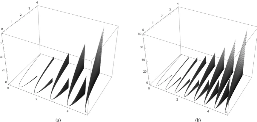
Fig. 2 provides us with the graphical illustration of the
C(f3;H) and C(f5;H) in this case. The values of these
integrals are the areas of the surfaces presented in plot (a) and (b), respectively.
In order to compute the limit value in Eq. 1 let us note, that in the considered case
Ak≤C(fk, H)≤Bk (5)
where
Ak = 2197(169[20k/13]−585[20k/13]2+ 980[20k/13]3)/184320k3
Bk = 2197(564 + 1939[20k/13] + 2355[20k/13]2+ 980[20k/13]3)/184320k3
(6) with [x] denoting the greatest integer less than or equal to x. Because the limit of bothAk, Bk asktends to infinity is the same and equales L1 = 6125/144, it is also the limit of
C(fk, H)that we have been looking for.
Now let us find the limit with the help of the Eq. 1. i.e. by computation of the value of the Young functional YF(H). For this purpose we need to know the classical Young measure generated by the ROSU(f). With the help of Corollary 4.1 one can easily receive the following formula for its density function:
g(y) = 4/(13√y)1[0,25/16)(y)
+2/(13√y)1[25/16,4)(y)
Thus the value of the Young functional in the considered case is the following (recall that the Young measure νx is
homogeneous in this case, so we can omit subscript ”x” in the denotations) :
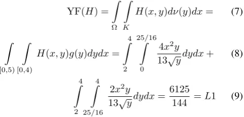
YF(H) = Z
Ω
Z
K
H(x, y)dν(y)dx= (7)
Z
[0,5)
Z
[0,4)
H(x, y)g(y)dydx=
4
Z
2 25/16
Z
0
4x2y
13√ydydx+ (8)
4
Z
2 4
Z
25/16
2x2y
13√ydydx=
6125
144 =L1 (9)
So, as it should be expected, the ”whole information” about the rapid oscillations in this case is contained in the classical Young measure and due to the Proposition 3.1 -can be revealed with the help of the Corollary 4.1. Because we are going to make use of this example as a kind of benchmark in our next considerations, let us also compute both the limit and the Young functional values for another Carath´eodory function, namely let H(x, y) = xcos(y). In this case little calculus shows thatC(f k;H)satisfy (5) with
Ak = [2016k/k13]2 (3 √
2π(F(2p2/π) +F(5/(2√2π)))+ 13√2π[20k/13](F(2p2/π) +F C(5/(2√2π))+ 8(sin(25/16)−sin(4)))
Bk = 1+[2016kk/213](13 √
2π[20k/13](F(2p2/π)+
F(5/(2√2π)) + 16√2π(F(2p2/π)+
F(5/(2√2π)) + 8(sin(25/16)−sin(4))) (10) where F denotes the special function known as the Fresnel
IAENG International Journal of Applied Mathematics, 48:4, IJAM_48_4_03
[image:4.595.309.550.432.548.2](a) (b)
Fig. 2: Graph of two exemplary surfaces - plot (a) and plot (b) - the area of which are, respectively, the values of the integrals C(f3;H)andC(f5;H). These integrals are elements of the sequence on the left-hand side of the Eq. 1
function that is given by the following integral:
F(z) = z Z
0
cos(πt2/2)dt
Again, the limits of bothAk, Bkare the same, so they are the same as the limit ofC(fk, H) in this case. It equals
L2 = (25√2π/13)(F(2p2/π) +F(5/(2√2π)) (11)
The same value can be obtain with the help of our result. Indeed, it is easy to check, that the integral (7) in the considered case takes on the form:
4
Z
2 25/16
Z
0
4xcos(y) 13√y dydx+
4
Z
2 4
Z
25/16
2xcos(y) 13√y dydx
and it is equal toL2.
Our example is relatively simple and ”smooth” - we were able to compute the limits explicitly. However even here one can notice the benefits resulting from our Proposition. It is quite clear that even in this case where the oscillations have such smooth nature, the computation of the limit ofC(fk, H) for more complex Carath´eodory functions could be much more difficult task than the calculation of the value of the Young functionalYF(H).
The possibility of derivation of explicit formulae for the density functions of classical Young measures is not the only benefit resulting from our Proposition 3.1. In many interesting cases explicit formulae for these densities cannot be found. For instance, if one wants to make use of Corollary 4.1 they have to obtain the inverses of f on particular subintervals of its domain, but it is not always possible. However in all such cases thanks to Proposition 3.1 one may use directly Monte Carlo simulations in order to evaluate values of the Young functionals.
The idea of the Monte Carlo simulation is well-known. Its main concept is to draw a sample Z1, Z2, ..., Zm of realizations of independent random variables with the same distribution as the random phenomenon under study. Based
on this sample, important information concerning stochastic characteristics of the examined distribution can be derived with the help of statistical-inference tools. Monte Carlo simulations are also frequently used to evaluate values of integrals in various situations. Because now we consider cases where the classical Young measure is not given ex-plicitly, we adopt this approach to evaluate Young functional
YF(H) = d R
c b R
a
H(x, y)dν(y)
dx. When the change of
integration order is possible, then this integral is equal to
YF(H) = b R
a d R
c
H(x, y)dx)
dν(y).
By Proposition 1, the Young measureν is the probability distribution of the random variable Y=f(U(a,b)). So, we may look at the Young-functional-value as the expected value
of the random variable d R
c
H(x, Y)dx and it is well-known
that it can be best-estimated by its empirical mean (i.e. the arithmetic mean of its randomly generated values). Thus we propose to make use of the following procedure YFE(H, f , a, b, c, d, N) to evaluate values of the Young functional:
•
Step 0: Set k= 1
Step 1: Set t=Random((a,b)) Step 2: Set y=f(t)
Step 3: Set z[k]=INT(H(x,y),x,c,d) Step 4: N times repeat Steps 1 to 3 Step 5: Set sample=(z[1],...,z[N]) Step 6: Set YF=Mean(sample) Step 7: Return YF
The above procedure is called with the following argu-ments: the formula that defines the Caratheodory function H, the formula for the function f that defines the ROSU and its domain, i.e. the interval [a,b), the domain [c,d) of the ROSU itself, and the size N of the sample that will be used to evaluate the Young functional value. The subroutine Random(I) returns a pseudorandom number generated ac-cording to the uniform probability distribution defined on an interval I. The subroutine INT(H(x,y), x,c,d) returns the value
IAENG International Journal of Applied Mathematics, 48:4, IJAM_48_4_03
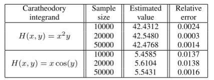
TABLE I: Results Of Monte Carlo Evaluations of the Young Functional Values for Problems Considered in Example 1
Caratheodory Sample Estimated Relative
integrand size value error
10000 42.4312 0.0024
H(x, y) =x2y 20000 42.5480 0.0003 50000 42.4768 0.0014
10000 5.4585 0.0137
H(x, y) =xcos(y) 20000 5.6104 0.0138
50000 5.5431 0.0016
of the integral d R
c
H(x, y)dx. Obviously the integration can be
done numerically, because when the subroutine is called, the value of y is already fixed, as it is set up at the Step 2. The usefulness of the Monte Carlo simulations in computation of the values of the Young functionals is supported by the data presented in Table I.
As one can see, the accuracy of the Monte Carlo evalua-tions are realy very good (let us recall that the true values are L1 andL2, given by (9) and (11), respectively). Other examples of the advantages resulting from the Monte Carlo approach to computation of Young functionals’ values can be found in [8].
The pseudocode of the procedure YFE presented in this section can be implemented in various ways. In our research we use the following version coded in Wolfram Mathematica 10.5 programming environment:
Mean[Table[
NIntegrate[H[x,f[RandomReal[{a,b}]]],
{x,c,d}],NN]]
where NN is the sample size, while the remaining symbols have an analogous meaning as in the description of the YFE.
Now, let us consider the following functionG:
G(y) = d Z
c
H(x, y)dx (12)
If the Caratheodory integrands are such that the functionG
has got known open formula valid for ally ∈(a, b), then a faster version of YFE can be obtain by changing the original Step 3 in the following way:
Step 3: Set z[k]=G(y)
In our exemplary problems, it can be actually done, so we made use of the following Wolfram Mathematica code:
Mean[Table[G[f[RandomReal[{a,b}]]]],NN]]
where, for the problems discussed in Example 1 G(y) = 125y/3 if H(x, y) = x2y and G(y) = 25 cos(y)/2 if
H(x, y) =xcos(y). Recall that in both cases the limits in integral (12) arec= 0, d= 5
We see that practical implementation of presented Monte Carlo evaluation procedure is very simple and taking into account the accuracy of the values we have obtained, it is also very competitive alternative tool for engineers.
VI. FINAL REMARK
The probability theory provides us with a number of different versions of the theorems concerning the probability distributions of functions of random variables and/or vectors.
As a consequence, various different rules for computing explicit formulae for the density functions of classical Young measures generated by ROSU(f) can also be obtained on the basis of the result stated in Proposition 3.1.
We are also sure that the same approach enables devel-opment of analogous results related to rapidly oscillating sequences with uniform representation which are defined on open and bounded subsets ofRd. In our opinion it is very promising direction of future research.
REFERENCES
[1] J.B. Bacani, and G. Peichl, ,,The Second-Order Eulerian Derivative of a Shape Functional of a Free Boundary Problem”,IAENG International Journal of Applied Mathematics, vol. 46, no. 4, pp.425–436, 2016. [2] J.M. Ball, ,,Mathematical Models of Martensitic Microstructure”,
Ma-terials Science and Engineering A378. pp. 61–69, 2004.
[3] J.M. Ball, and R.D. James, ”Fine Phase Mixtures as Minimizers of Energy”,Archive for Rational Mechanics and Analysis, 100, pp.13–52, 1987.
[4] P.Billingsley, Convergence of Probability Measures, John Willey & Sons, 1968.
[5] M. Chipot, and C. Collins, and D. Kinderlehrer, ,,Numerical Analysis of Oscillations in Multiple Well Problems”, Numerische Mathematik
70, pp 259–282, 1995.
[6] A.Z. Grzybowski, and P. Puchała, ”On general characterization of Young measures associated with Borel functions”, preprint, arXiv: 1601.00206v2, submitted.
[7] A.Z. Grzybowski, and P. Puchała, ”On Classical Young Measures Generated by Certain Rapidly Oscillating Sequences,” Lecture Notes in Engineering and Computer Science: Proceedings of The World Congress on Engineering and Computer Science 2017, 25-27 October, 2017, San Francisco, USA, pp889-892
[8] A.Z. Grzybowski, and P. Puchała, ” Monte Carlo Simulation in the Evaluation of the Young Functional Values”, Proceedings of IEEE 14th International Scientific Conference on Informatics, Poprad, (eds. Novitzka, S. Korecko, A. Szakal), New York 2017, pp221-226 [9] W. Han, and B.D. Reddy, ,,Computational Plasticity: the Variational
Basis and Numerical Analysis”,Computational Mechanics Advances2, pp. 283–400, 1995.
[10] G. Hou, and G. Wang, and Z. Pan, and B. Huang, and H. Yang, and T. Yu, ”Image Enhancement and Restoration: State of the Art of Variational Retinex Models,”IAENG International Journal of Computer Science, vol. 44, no.4, pp445–455, 2017.
[11] S. M¨uller, ”Variational Models for Microstructure and Phase Tran-sitions”, inCalculus of variations and geometric evolution problems, Hildebrandt, S., Struwe, M. (editors), Lecture Notes in Mathematics Volume 1713, Springer Verlag, Berlin Heidelberg, Germany 1999. [12] P. Puchała,“An elementary method of calculating Young measures in
some special cases,”Optimization, vol. 63 no.9, pp.1419–1430, 2014. [13] P. Pedregal, Variational Methods in Nonlinear Elasticity, SIAM,
Philadelphia 2000.
[14] T. Roub´ıˇcek, Relaxation in Optimization Theory and Variational Calculus, Walter de Gruyter, Berlin, New York, 1997.
[15] L.C. Young,“ Generalized curves and the existence of an attained absolute minimum in the calculus of variations,”Comptes Rendus de la Soci´et´e des Sciences et des Lettres de Varsovie, classe III vol. 30, pp. 212–234, 1937.
[16] L.C. Young, ”Generalized surfaces in the calculus of variations”,Ann. Math.vol. 43, part I: pp. 84–103, part II: pp. 530–544, 1942.