Weak Dependence on Initialization
in Mixture of Linear Regressions
Ryohei Nakano and Seiya Satoh
Abstract—This paper examined how initial values of a learning algorithm influence the performance of mixture of linear regressions (MoLR). MoLR employs the EM algorithm as a learning algorithm. Our experiments used two kinds of artificial data and one real dataset. Experiments using artificial data showed MoLR discovered the original lines from data containing Gaussian or t-distribution noise. Moreover, almost all our experiments showed the best solution can be easily found with any initialization method. This suggests MoLR may have rather weak dependence on initialization.
Index Terms—mixture model, mixture of regressions, EM algorithm, clustering, information criterion
I. INTRODUCTION
This paper examines how initial values of the learning, here the EM algorithm [1], influence the final performance of mixture of linear regressions (MoLR).
First, mixture of regressions (MoR) is briefly reviewed. Given multivariate data, consider a regression problem, that is, try to explain the behavior of a target variable using ex-planatory variables. It may happen that any single regression function cannot explain well. There can be several reasons for this: a lack of explanatory variables, the intrinsic randomness of the target variable, and so on. When data arise from heterogeneous contexts, it is reasonable to introduce MoR.
There can be two types of the mixture. One ishard mixture
and the other issoft mixture. In the former each data point is exclusively classified into one of the classes, while in the latter each data point probabilistically belongs to every class. Hard mixture has been called regression clustering [2], [3] or cluster-wise (linear) regression [4]. Soft mixture has been simply called mixture of regressions.
Research on hard MoR has been less popular, while soft MoR has the solid background developed as finite mixture models. Finite mixture models provide a flexible tool for modeling data that arise from heterogeneous populations. The book by McLachlan and Peel [5] contains a com-prehensive review of finite mixture models. Leisch gave a general framework for MoR in the R statistical computing environment [6]. Huang, Li, and Wang investigated MoR by employing kernel regression [7]. The book by Bishop [8] contains mixture models including MoLR.
Next, how a learning method for MoLR depends on the initialization is briefly reviewed. As a learning method, hard MoLR usually employs Sp¨ath’s exchange algorithm [4], while soft MoR usually employs the EM algorithm
This work was supported by Grants-in-Aid for Scientific Research (C) 16K00342.
R. Nakano is with the Department of Computer Science, Chubu Univer-sity, 1200 Matsumotocho, Kasugai 487-8501, Japan. [email protected] S. Satoh is with National Institute of Advanced Industrial Sci-ence and Technology, 2-4-7 Aomi, Koto-ku, Tokyo, 135-0064, Japan. [email protected]
[1]. It is known that the success of the Sp¨ath’s exchange algorithm depends heavily on the initial configuration [2]. Qian and Wu [3] proposed a method to generate an initial configuration for hard MoLR. On the other hand, the local optimality of the EM algorithm is well known, and in general its performance depends heavily on its initial values. To overcome its optimality, several EM variants have been proposed, such as DAEM [9] and SMEM [10]. Thus, the initial configuration for the EM algorithm may play a large role in soft MoLR.
This paper examines how initial values of the EM al-gorithm influence the performance of soft MoLR. Section 2 explains the framework of soft MoLR, and Section 3 describes initialization and model selection. In the initial-ization we propose a new method to generate regression-oriented initial values for MoLR, and in model selection we explain information criterion to evaluate the desirability of MoLR candidates. Then Section 4 describes our experiments performed to examine how initial values of the EM algorithm influence the performance of MoLR using two kinds of artificial data and one real dataset.
II. MIXTURE OFLINEARREGRESSIONS(MOLR)
Following Bishop [8], this section explains the framework of soft MoLR, which employs the EM algorithm [1] as a learning method.
We consider a mixture ofC linear regression models. Let
x= (x1,· · ·, xK)T be explanatory variables, and y denotes a target variable. Since we consider a constant term in each regression function, we extend a vector of explanatory variables asxe= (1, x1,· · ·, xK)T.
We assume the value of y is generated by adding a Gaussian noise to a value of linear regression function
f(x|wc) with wc as its weight vector. A linear regression function of classcis defined as follows.
f(x|wc) = wTc xe (1)
Although Bishop assumes the common error variance (equivalently, a precision parameter) for all classes, we introduce individual variance for each class to enhance the fitting capability of the model. That is, for classc, an error
εc follows the Gaussian with mean 0 and variance σc2.
εc ∼ N(0, σ2c) (2)
Classcis a latent variable and cannot be observed. The target variabley follows the following distribution.
y ∼ N(f(x|wc), σ2c) (3)
Letπcbe the mixing coefficient of classc. Then, the density of complete-data is described as follows.
Hereg(u|m, s2)denotes a density function whereufollows
one-dimensional Gaussian with meanm and variances2.
g(u|m, s2) = √1 2π s exp
(
− (u−m)2 2s2
)
(5)
The density of incomplete-data is written as follows.
p(y|θ) = C
∑
c=1
p(y, c|θc) = C
∑
c=1
πc gc(y|f(x|wc), σ2c) (6) Here θ is a vector comprised of all parameters, while θc is a vector of classc parameters.
θ= (θT1,· · ·,θTc,· · ·,θTC)T, θc = (πc, wTc, σ
2
c) T
(7)
Now the posterior probability is written as follows, which indicates the probability that y belongs to classc.
P(c|y,θ) = ∑p(y, c|θ) cp(y, c|θ)
(8)
Given data D={(xµ, yµ), µ= 1,· · ·, N}, the incomplete-data log likelihood is defined as below.
L(θ) =
N
∑
µ=1
log p(yµ|θ) (9) When we employ the EM algorithm to estimate MoLR parameters, the Q-function to maximize is shown as below. Here θ(t) denotes the estimate at the t step of the EM algorithm, and letfµ
c ≡f(xµ|wc).
Q(θ|θ(t)) = ∑ µ
∑
c
P(c|yµ,θ(t)) log p(yµ, c|θ)
= ∑
µ
∑
c
Pcµ(t) log(πc gc(yµ|fcµ, σc2))
= ∑
µ
∑
c
Pcµ(t)
(
logπc− 1
2log(2π)
−logσc−
(yµ−fµ c)22 2σ2
c
)
(10)
In the above, we use the following for brevity.
Pcµ(t) ≡ P(c|yµ,θ(t)) = π
(t)
c g
µ(t)
c
∑
cπ
(t)
c g
µ(t)
c
(11)
wheregµc(t)≡gc(yµ|fcµ(t), σ
2(t)
c ) (12)
When we maximize the Q-function, we use the Lagrange method since there is an equality constraint∑cπc= 1. The Lagrangian function can be written as follows with λ as a Lagrange multiplier.
J = Q(θ|θ(t))−λ
( ∑
c
πc−1
)
(13)
The necessary condition for a local maximizer is shown below.
∂J ∂πc
= ∑
µ
Pcµ(t)/πc−λ= 0 (14)
∂J ∂wc
= ∑
µ
Pcµ(t)(y
µ−fµ c)
σ2
c
∂fµ c
∂wc
=0 (15)
∂J ∂σc
= ∑
µ
Pcµ(t)
(
−1
σc +(y
µ−fµ c)2
σ3
c
)
= 0 (16)
Since we have λ = N from eq.(14) and the equality constraint, a new estimate ofπc is given below.
πc(t+1) = 1
N
∑
µ
Pcµ(t) (17)
From eq.(16) a new estimate ofσc2 is given below.
(σ2c)(t+1) = ∑ µ
Pcµ(t)(yµ−fcµ)2
/ ∑
µ
Pcµ(t) (18)
From eq.(15) we obtain a new estimate ofwcby solving the following.
∑
µ
Pcµ(t)(yµ−fcµ)∂f µ c
∂wc
=0 (19)
Here in this paper we consider linear regression models as mixture elements. So by substituting eq.(1) into the above, we have the following.
∑
µ
Pcµ(t)(yµ−wTcxeµ)xeµ=0 (20) This formula is transformed in succession as below.
∑
µ
Pcµ(t)(wcTxeµ)xeµ = ∑ µ
Pcµ(t)yµ xeµ ∑
µ
Pcµ(t)xeµ(exµTwc) =
∑
µ
Pcµ(t)yµ xeµ ∑
µ
Pcµ(t)(xeµexµT)wc =
∑
µ
Pcµ(t)yµ xeµ (21) Here data of explanatory variables is expressed as the fol-lowingN×(K+ 1)matrix, and data of a target variable is expressed as the followingN×1vector.
f
X = (xe1,· · ·,xeµ,· · ·,xeN)T (22)
y = (y1,· · ·, yµ,· · ·, yN)T (23) For each class c, we consider N × N diagonal matrix
S(ct) =diag(P µ(t)
c ), whoseµ-th diagonal element is Pcµ(t). Then eq.(21) can be written as follows.
(fXTSc(t)fX)wc =Xf T
S(ct)y (24) When there is the inverse matrix of the above equation, we have the following new estimate of weights.
w(ct+1)= (fXTS(ct)fX)−1fXTS(ct)y (25) III. INITIALIZATION ANDMODELSELECTION
A. Initialization of MoLR
We consider two methods for the initialization of MoLR. One is random initialization (R init), where each data point is randomly assigned to one of the classes.
The other is a new method which classifies data points into clusters taking into account the height of target values. The method is called height-sensitive initialization (HS init). The procedure goes as follows. First, perform linear regression using all data points and classify them into upper, lower, and remaining groups. Then the upper group is grouped into two setsU1andU2, and the lower group is also grouped into
L1 and L2. The remaining groupR consists of data points
this method is to separate data into upper, middle, and lower groups; such separation is expected be effective to make good initial configurations of MoLR.
HS initialization making 2 classes:
step 1. Perform linear regression using all data points. step 2. If a data point is more than toleranceδ higher than the regression plane, it is assigned to the set U, and if the point is more than δ lower than the plane, it is assigned to
L, and if it is near the plane, it is assigned toR.
step 3. U is grouped into two sets U1 and U2, and L is
grouped into L1 and L2 as well. We employ Kmeans [11]
for this clustering.
step 4. By combining four sets except seemingly less relevant
R, we make the following 7 initial configurations.
N o.1 : {U1, U2} ∪ {L1, L2}
N o.2 : {U1, L1} ∪ {U2, L2}
N o.3 : {U1, L2} ∪ {U2, L1}
N o.4 : {U1} ∪ {U2, L1, L2}
N o.5 : {U2} ∪ {U1.L1, L2}
N o.6 : {L1} ∪ {U1, U2, L2}
N o.7 : {L2} ∪ {U1, U2, L1}
HS initialization making 3 classes:
steps 1, 2 and 3 are the same as the above.
step 4. By combining all five sets with (1,2,2) pattern, we make the 15 initial configurations such as {R}∪{U1, U2}∪
{L1, L2} and{R} ∪ {U1, L1} ∪ {U2, L2}.
B. Model Selection
In the context of MoR, we consider many candidates of mixture models; thus, we need a criterion to evaluate the desirability of each candidate and to select the best mixture model. For this purpose we make use of information criterion. Although many information criteria have been pro-posed so far, we employ the Bayesian information criterion BIC [12], because BIC stably showed good performance in our experiments on MLP model selection [13]. BIC was proposed for regular models, but it also works rather well for singular models such as multilayer perceptrons (MLPs). Let p(x|w) be a learning model with parameter vector
w. Given data {xµ, µ = 1,· · ·, N}, the log-likelihood is defined as follows:
LN(w) = N
∑
µ=1
logp(xµ|w). (26) Letwb be a maximum likelihood estimator. BIC is obtained as an estimator of free energyF(D)shown below. Herep(D) is called evidence andp(w)is a prior distribution ofw.
F(D) = −logp(D), (27)
p(D) =
∫
p(w) N
∏
µ=1
p(xµ|w) dw (28)
BIC is derived using the asymptotic normality and Laplace approximation.
BIC = −2LN(wb) +MlogN = −2
N
∑
µ=1
logp(xµ|wb) +MlogN (29)
BIC can be calculated using only one point estimatorwb. HereM is the number of parameters.
As another standpoint, total sum of squares (TSS) indicates how much variation the data have, residual sum of squares (RSS) indicates the discrepancy between the data and the estimates, and explained sum of squares (ESS) indicates how well a regression model represents the data. These quantities satisfy the relation TSS = ESS + RSS. Thus, ESS/TSS indicates goodness of fit for a regression model.
IV. EXPERIMENTS
We performed experiments to examine how initial values of the EM algorithm influence the performance of MoLR using two kinds of artificial data and one real dataset. As artificial data, we utilized Qian-Wu’s one-dimensional data [3]. Datasets were generated using the following two linear functions: for each dataset 70 and 50 points were generated for y1 and y2 respectively with one of two kinds of noise
added.
y1= 2 + 8x1, y2= 1 + 5x1 (30)
Moreover, R init was repeated 50 times for each dataset.
A. Experiment using Artificial Data 1
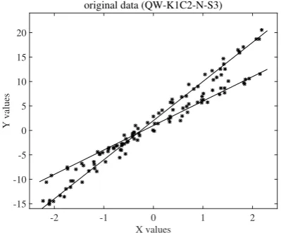
[image:3.595.320.520.424.590.2]In artificial data 1, standard Gaussian noise N(0,1) was added to the lines shown in eq.(30). We generated five datasets for artificial data 1.
Figure 1 shows one dataset, depicting two original lines and 120 data points.
-2 -1 0 1 2
X values -15
-10 -5 0 5 10 15 20
Y values
original data (QW-K1C2-N-S3)
Fig. 1. Two Original Lines and Qian-Wu Data Generated with Gaussian N(0,1) Noise and Seed 3
For all five datasets, criterion BIC for 2 classes (C=2) was smaller than those for C=3. Figure 2 shows the best results of our soft MoLR of C=2 for Fig. 1 dataset. We can see two obtained lines fit well to data points.
Table I compares the original parameters with parameters obtained by our soft MoLR and hard MoLR by Qian-Wu [3]. The table shows both soft and hard MoLRs found good estimates. Moreover both HS and R inits for soft MoLR got much the same results.
Figure 3 shows the best results of soft MoLR of C=3 for Fig. 1 dataset. Three lines somehow cover all data points.
-3 -2 -1 0 1 2 3 X values
-20 -15 -10 -5 0 5 10 15 20 25
Y values
MOR results (2 classes) init config:6
Fig. 2. Two Lines of the Best MoLR Model of 2 Classes for Qian-Wu Data Generated with Gaussian N(0,1) Noise and Seed 3
TABLE I
ORIGINAL ANDOBTAINEDPARAMETERS
w1 w2
Original (2, 8)T (1, 5)T soft MoLR(HS, C=2) (2.0408, 8.0410)T (0.8076, 5.2077)T
soft MoLR(R,C=2) (2.0409, 8.0411)T (0.8076, 5.2077)T Qian-Wu(C=2) [3] (2.12, 8.02)T (0.76, 5.11)T
6 and 7 show histograms of BIC obtained by MoLR using R init. These figures show that the best solution of C=2 was better than that of C=3. Moreover, for the best model (C=2), HS init found the best solution 4 times out of 7, and R init found the best solution 48 times out of 50. This means for the best model the best solution can be easily found with any initialization.
B. Experiment using Artificial Data 2
In artificial data 2, t-distribution noiset(3)was added to the lines shown in eq.(30). We generated five datasets for artificial data 2.
Figure 8 shows one dataset, depicting two original lines and 120 data points. Compared with Fig. 1, data points are more widely scattered around the lines.
For five datasets, the true model C=2 was selected four times out of five. In Qian-Wu [3] incorrect C=3 was more
-3 -2 -1 0 1 2 3
X values -20
-15 -10 -5 0 5 10 15 20 25
Y values
MOR results (3 classes) init config:14
Fig. 3. Three Lines and the Best MoLR Model of 3 Classes for Qian-Wu Data Generated with Gaussian N(0,1) Noise and Seed 3
220 230 240 250 260 270 280 BIC
0 1 2 3 4
frequency
Histram of BIC with QW_N_S3_HS_C2
Fig. 4. BIC Histogram for QW Data with HS Init, 2 Classes, and Gaussian N(0,1) Noise
220 230 240 250 260 270 280 BIC
0 1 2 3 4 5 6 7
frequency
Histram of BIC with QW_N_S3_HS_C3
Fig. 5. BIC Histogram for QW Data with HS Init, 3 Classes, and Gaussian N(0,1) Noise
220 230 240 250 260 270 280 BIC
0 10 20 30 40 50
frequency
Histram of BIC with QW_N_S3_R_C2
Fig. 6. BIC Histogram for QW Data with R Init, 2 Classes, and Gaussian N(0,1) Noise
220 230 240 250 260 270 280 BIC
0 5 10 15 20 25
frequency
Histram of BIC with QW_N_S3_R_C3
Fig. 7. BIC Histogram for QW Data with R Init, 3 Classes, and Gaussian N(0,1) Noise
frequently selected than C=2. Figure 9 shows the best results of our soft MoLR of C=2 for Fig. 8 dataset. We can see much the same lines as original were obtained.
Table II compares the original parameters with parameters obtained by soft MoLR. The table shows soft MoLR found rather exact estimates. Both HS and R inits reached exactly the same results.
TABLE II
ORIGINAL ANDOBTAINEDPARAMETERS
w1 w2
Original (2, 8)T (1, 5)T soft MoLR(HS, C=2) (1.5266, 8.1031)T (1.1869, 5.1504)T
soft MoLR(R, C=2) (1.5266, 8.1031)T (1.1869, 5.1504)T
Figure 10 shows the best results of soft MoLR of C=3 for Fig. 8 dataset. Two lines out of three almost overlap each other.
Figures 11 and 12 show histograms of BIC values obtained
-2 -1 0 1 2
X values -15
-10 -5 0 5 10 15 20
Y values
original data (QW-K1C2-T-S1)
-3 -2 -1 0 1 2 3 X values
-20 -15 -10 -5 0 5 10 15 20 25
Y values
MOR results (2 classes) init config:4
Fig. 9. Two Lines of the Best MoLR Model of 2 Classes for Qian-Wu Data Generated with t-dist t(3) Noise and Seed 1
-3 -2 -1 0 1 2 3
X values -20
-15 -10 -5 0 5 10 15 20 25
Y values
MOR results (3 classes) init config:6
Fig. 10. Three Lines of the Best MoLR Model of 3 Classes for Qian-Wu Data Generated with t-dist t(3) Noise and Seed 1
by our MoLR using HS init, while Figs. 13 and 14 show BIC obtained by MoLR using R init. These figures show that the best solution of C=2 was surely better than that of C=3. Moreover, for the best model (C=2), HS init found the best solution 4 times out of 7, and R init found the best solution 44 times out of 50. Again this means that for the best model we can easily find the best solution with any initialization.
250 260 270 280 290 300 BIC
0 1 2 3 4
frequency
Histram of BIC with QW_T_S1_HS_C2
Fig. 11. BIC histogram for QW Data with HS Init, 2 Classes, and t-dist t(3) Noise
250 260 270 280 290 300 BIC
0 0.5 1 1.5 2 2.5 3
frequency
Histram of BIC with QW_T_S1_HS_C3
Fig. 12. BIC histogram for QW Data with HS Init, 3 Classes, and t-dist t(3) Noise
C. Experiment using Real Data
As real data we used Abalone dataset from UCI Machine Learning Repository. We selected this because any single regression function cannot fit well. The dataset has seven
250 260 270 280 290 300 BIC
0 10 20 30 40 50
frequency
Histram of BIC with QW_T_S1_R_C2
Fig. 13. BIC histogram for QW Data with R Init, 2 Classes, and t-dist t(3) Noise
250 260 270 280 290 300 BIC
0 10 20 30 40 50
frequency
Histram of BIC with QW_T_S1_R_C3
Fig. 14. BIC histogram for QW Data with R Init, 3 Classes, and t-dist t(3) Noise
numerical explanatory variables and the number of data points is 4177 (N =4177).
As a powerful single regression model, we employ mul-tilayer perceptron (MLP) and a learning method called SSF (singularity stairs following) [14], [15]. SSF successively learns MLP models to find very excellent solutions making good use of singular regions. SSF guarantees monotonic decrease of training errors, thus is very suited to model selection.
Figure 15 shows BIC values for Abalone dataset by SSF. The figure indicatesJ =7 is the best model. BIC atJ =7 was 15,600. Multiple correlation coefficient at J =7 is 0.7940; thus, the coefficient of determination is 0.6304, which is not so high.
2 4 6 8 10
J
1.5551.56 1.565 1.57 1.575 1.58 1.585 1.59
BIC
104
Fig. 15. BIC for Abalone by SSF
2 4 6 8 10
J
0.360.37 0.38 0.39 0.4 0.41 0.42 0.43 0.44 0.45 0.46
MSE
tr
Fig. 16. Training MSE for Abalone by SSF
monotonically. MSE at J =7 was 0.3695, while minimum MSEs of best MoLR (C=2) and best MoLR (C=3) were 0.2692 and 0.2018 respectively. This indicates MoLR (C=3) could fit better than MoLR (C=2), and a mixture of two or three linear regressions could fit better than a single MLP with SSF.
Table III compares BIC values and goodness of fit ESS/TSS for different regression models and different ini-tialization methods. We can see the init methods of MoLR made little difference. Moreover, MoLR (C=3) had smaller BIC than MoLR (C=2), and MoLR had smaller BIC than MLP with SSF. MoLR (C=3) showed the highest goodness of fit, higher than very powerful single nonlinear regression model MLP with SSF.
TABLE III BICFORABALONEDATASET
Model & Method BIC ESS/TSS MoLR (C=2) with HS Init 3644 0.7291
MoLR (C=2) with R Init 3644 0.7308 MoLR (C=3) with HS Init 3523 0.7982 MoLR (C=3) with R Init 3523 0.7960 MLP (J=7) with SSF 15600 0.6304
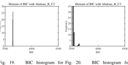
Figures 17 and 18 show histograms of BIC obtained by MoLR using HS init, while Figs. 19 and 20 show BIC obtained by MoLR using R init. These figures show that the best solution of C=3 was better than that of C=2. Moreover, for the best model (C=3), HS init found the best solution 7 times out of 15, and R init found it 35 times out of 50. Again this means that for the best model (C=3) we can easily find the best solution with any initialization.
3500 4000 4500 BIC
0 0.5 1 1.5 2
frequency
[image:6.595.47.277.438.736.2]Histram of BIC with Abalone_HS_C2
Fig. 17. BIC histogram for Abalone Data with HS Init and 2 Classes
3500 4000 4500
BIC 0
1 2 3 4 5 6 7
frequency
Histram of BIC with Abalone_HS_C3
Fig. 18. BIC histogram for Abalone Data with HS Init and 3 Classes
3500 4000 4500
BIC 0
5 10 15 20 25 30
frequency
[image:6.595.49.274.590.704.2]Histram of BIC with Abalone_R_C2
Fig. 19. BIC histogram for Abalone Data with R Init and 2 Classes
3500 4000 4500
BIC 0
5 10 15 20 25 30 35
frequency
Histram of BIC with Abalone_R_C3
Fig. 20. BIC histogram for Abalone Data with R Init and 3 Classes
V. CONCLUSION
This paper examined how initial values of the EM algo-rithm influence the performance of soft mixture of linear
regressions (MoLR). Our experiments used two kinds of artificial data and one real dataset. Experiments using ar-tificial data showed soft MoLR successfully discovered the original lines from data containing Gaussian or t-distribution noise. Experiments using real dataset showed soft MoLR had smaller BIC and higher goodness of fit than single MLP. This shows the potential of MoLR. Moreover, almost all our experiments showed the best solution can be found with more than 50 % using any of two initializations. This may suggest soft MoLR may have rather weak dependence on initialization.
In the future we plan to investigate more to verify the plausibility of this tendency and further extend MoLR to nonlinearity.
REFERENCES
[1] A. P. Dempster, N. M. Laird, and D. B. Rubin, “Maximum-likelihood from incomplete data via the EM algorithm,”J. Royal Statist. Soc. Ser. B, vol. 39, pp. 1–38, 1977.
[2] NCSS, “Regression clustering,” NCSS Statistical Software Documen-tation, Tech. Rep. Chapter 449, pp.1–7, 2013.
[3] G. Qian and Y. Wu, “Estimation and selection in regression clustering,”
European Journal of Pure and Applied Mathematics, vol. 4, no. 4, pp. 455–466, 2011.
[4] H. Sp¨ath, “Algorithm 48: A fast algorithm for clusterwise linear regression,”Computing, vol. 29, pp. 175–181, 1982.
[5] G. J. McLachlan and D. Peel,Finite mixture models. John Wiley & Sons, 2000.
[6] F. Leisch, “FlexMix: A general framework for finite mixture models and latent class regression in R,” Journal of Statistical Software, vol. 11, no. 8, pp. 1–18, 2004.
[7] M. Huang, L. Runze, and W. Shaoli, “Nonparametric mixture of regression models,” Journal of the American Association, vol. 108, no. 503, pp. 929–941, 2013.
[8] C. M. Bishop,Pattern recognition and machine learning. Springer, 2006.
[9] N. Ueda and R. Nakano, “Deterministic annealing EM algorithm,”
Neural Networks, vol. 11, no. 2, pp. 271–282, 1998.
[10] N. Ueda, R. Nakano, Z. Ghahramani, and G. E. Hinton, “SMEM algorithm for mixture models,” Neural Comput., vol. 12, no. 9, pp. 2109–2128, 2000.
[11] Y. Linde, A. Buzo, and R. M. Gray, “An algorithm for vector quantizer design,”IEEE Trans. on Communications, vol. 28, no. 1, pp. 84–95, 1980.
[12] G. Schwarz, “Estimating the dimension of a model,” Annals of Statistics, vol. 6, pp. 461–464, 1978.
[13] S. Satoh and R. Nakano, “How new information criteria WAIC and WBIC worked for MLP model selection,” inProc. of 6th International Conf. on Pattern Recognition Applications and Methods (ICPRAM), 2017, pp. 105–111.
[14] ——, “Fast and stable learning utilizing singular regions of multilayer perceptron,”Neural Processing Letters, vol. 38, no. 2, pp. 99–115, 2013.