Maximum Likelihood Under Response Biased Sampling

Maximum Likelihood Under Response Biased Sampling

Raymond Chambers, Alan Dorfman, Suojin Wang

Abstract

Informative sampling occurs when the probability of inclusion in sample depends on the value of the survey response variable. Response or size biased sampling is a particular case of informative sampling where the inclusion probability is proportional to the value of this variable. In this paper we describe a general model for response biased sampling, which we call array sampling, and develop maximum likelihood and estimating equation theory appropriate to this situation. The Missing Information Principle (MIP) (Orchard and Woodbury, 1972) yields one (indirect) approach to likelihood based survey inference (Breckling et al 1994). Some have questioned its applicability in the case of informative sampling, because of the way it conditions on the given sample. In this paper we describe a direct approach and show that it and the MIP-based approach lead to identical results under array sampling. Comparison is made to the weighted likelihood based approach described in Krieger and Pfeffermann (1992). Extensions to the theory are also explored.

Maximum Likelihood Under Response Biased Sampling

By RAYMOND L. CHAMBERS(1)

University of Southampton, Southampton, UK

ALAN H. DORFMAN

Bureau of Labor Statistics, Washington, USA

and SUOJIN WANG

Texas A&M University, College Station, USA

April 2000

(1) Address for correspondence: Department of Social Statistics

University of Southampton

Highfield

Southampton SO17 1BJ

SUMMARY

Informative sampling occurs when the probability of inclusion in sample depends on the value

of the survey response variable. Response or size biased sampling is a particular case of

informative sampling where the inclusion probability is proportional to the value of this variable.

In this paper we describe a general model for response biased sampling, which we call array

sampling, and develop maximum likelihood and estimating equation theory appropriate to this

situation. The Missing Information Principle (MIP) (Orchard and Woodbury, 1972) yields one

(indirect) approach to likelihood based survey inference (Breckling et al 1994). Some have

questioned its applicability in the case of informative sampling, because of the way it conditions

on the given sample. In this paper we describe a direct approach and show that it and the

MIP-based approach lead to identical results under array sampling. Comparison is made to the

weighted likelihood based approach described in Krieger and Pfeffermann (1992). Extensions

to the theory are also explored.

Key Words: FINITE POPULATION, SUPERPOPULATION, INCLUSION

PROBABILITIES, MISSING INFORMATION PRINCIPLE, SCORE

FUNCTION, ESTIMATING EQUATION, WEIGHTED DISTRIBUTION

1.

Introduction

Consider the following situation. A population of N independent and identically distributed

realisations of a random variable X, with density f(x) indexed by an unknown parameter θ, is

sampled informatively. That is, the sampling method uses knowledge about the population

realisations of X to randomly determine which population units to include in the sample.

Unfortunately, the analyst (who wishes to make an inference about θ) only has access to the

sample values of X, plus a limited amount of information about the sampling method, in the form

of the value ξ of another parameter which, together with the (unknown) population values of X,

completely determines the distribution of the outcomes of the sampling process. It is assumed

that the analyst “knows” the functional form of the population density f, as well as enough

about the sample design to specify the conditional distribution (given X) of the (random) sample

inclusion indicator I.

The analyst wishes to estimate the value of θ on the basis of the available “data” (i.e. the sample

values of X and the value of ξ). He/she can then proceed in one of two ways.

(a) On the basis of knowledge of the population density f of X and the distribution of I

given X, the analyst can determine the “sampling density” f_s(x) of X. That is, the distribution of sample values of X obtained by repeated draws from the JOINT

population distribution of X and I. Operationally, this can be visualised as the

distribution of sample values of X obtained by a two step process: (i) generate N iid

population values of X from the density f(x) and index them as x₁, x₂, .., x_N; (ii) on the basis of these values, draw a sample s of n “labels” from the population index set {1, 2,

..., N} using the informative sampling method (which depends only on the known ξ and

whose outcome is s above. Note that knowledge of S is equivalent to knowledge of I_N. Clearly the distribution of X_S will NOT, in general, be the same as the distribution of n randomly chosen values of X. The task facing the analyst therefore is to determine the

distribution of X_S. Suppose this distribution can also be modelled, and in such a way that the only unknown in this distribution is the value of another parameter, say ω, which

is related, in a known way, to both θ and ξ. Provided the usual regularity conditions are

satisfied, it is clear that the sample values in X_S can be used to determine the MLE for ω, and consequently the MLE for θ obtained via invariance and the known relationship

between ω, θ and ξ. We refer to this approach as “sample-based” maximum likelihood.

(b) The analyst can use methods described in Breckling et al (1994) which, in the sampling

context, apply the Missing Information Principle (MIP) (Orchard and Woodbury 1972);

see also Chambers, Dorfman, and Wang (1998). That is, he/she can write down the score

function for θ generated by X_N and S, and then obtain the sample-based score function for θ by taking the conditional expectation of this population-based score given Sand

the sample values of X. The MLE for θ is obtained by setting this score to zero and

solving for θ. The essence of this approach is that, in taking the above conditional

expectation, there is no need to “model” the distribution of X_S, since this is replaced by a function dependent on the joint distribution of X_s and S, where sis the index set corresponding to the non-missing values in the population [i.e. sis the realization of S].

We refer to this approach as “MIP-based” maximum likelihood.

Both (a) “sample-based” likelihood and (b) “MIP-based” maximum likelihood are firmly

grounded in probability theory, and therefore must in principle lead to the same maximum

likelihood estimator, irrespective of whether the sampling method is informative or not. However,

this equivalence is not especially clear in the case of informative sampling. Consequently it is of

interest to explicitly demonstrate it for a method of informative sampling that has wide

In the following section we therefore introduce a simple method of informative sampling, which

we refer to as array sampling, and develop both the sample-based and MIP-based ML

estimating equations that arise. We show that under array sampling both sample-based and MIP

approaches lead to the same MLE for the parameter θ of interest. By way of comparison, in

Section 3 we develop the weighted distribution maximum likelihood estimator (WDMLE) for

this case. This estimator was introduced by Krieger and Pfeffermann (1992) specifically for

informative sampling. We show that under array sampling the WDMLE in fact corresponds to

an approximation to the MLE. Furthermore it is an approximation that can be inefficient in some

situations. In Section 4 we go on to generalise the definition of the MIP approach to arbitrary

estimating equations. In particular, we show that under array sampling a MIP-based estimating

equation for a population mean based on an unbiased population level estimating equation for

this parameter remains unbiased. Section 5 then concludes the paper with some discussion of

extensions and potential further research in this area.

2.

MLE under Array Sampling

The following sampling method, which we refer to as array sampling from now on, provides a

context for the theory developed in this paper. It can be taken as a first order model for draw by

draw with replacement informative sampling from a finite population of size N. It also

approximates the behaviour of systematic sampling applied to a randomly ordered population.

With an extension to “ragged array sampling” (see Section 5), it approximates the without

replacement sampling scheme proposed in Rao, Hartley and Cochran (1962) where the size

measure is in fact the survey variable of interest.

Consider a population which can be represented as an n × M array [X_{i j}] of iid realisations of a nonnegative random variable X, with density f(x) indexed by an unknown parameter θ. The

overall population size is thus N = nM. For simplicity we assume θ is scalar, although the

generalisation to the vector case is straightforward as illustrated in Example 2 below. Array

random variables {A_i, i = 1, 2, .., n}, each taking values over the integers between 1 and M, and such that, for j = 1, .., M

pr A

(

i = j Xi k;k =1,2,L, M

)

=

ξ +X_{i j}

Mξ +T_i (1)

where ξ > 0 is a known constant and T_i is the sum of X-values in row i of the array.

Our sample data then consist of the observed values of A_i, together with the values {

XiA_i; i=1,2,L, n }. That is, the values of Ai determine the outcome of an informative sampling

mechanism. Our objective is to compute the MLE for θ on the basis of these sample data.

To start, we adopt the sample-based likelihood approach. Clearly, the sample values

{

XiA_i; i=1,2,L, n } are independently distributed. Let ∆ be a small positive increment, with ∆x

= (x, x +∆). Then

pr X_iA i ∈∆x

(

)

= pr A

(

_i = j, X_ij∈∆_x

)

j=1 M

∑

=pr X

(

_ij∈∆_x

)

pr A

(

_i = j X_ij∈∆_x

)

j=1 M

∑

=pr X

(

_ij∈∆_x

)

pr A_i = j X_ij∈∆_x, X_ik

k≠j M

∑

=u

⎛ ⎝

⎜ ⎞

⎠ ⎟ f(u)du

∫

j=1 M

∑

=pr X

(

_ij∈∆_x

)

M ξ +x

Mξ +x+uf(u)du

∫

+o(∆)

=Mpr X

(

_ij∈∆_x

)

(

ξ +x

)

E 1 Mξ + x+U

⎛ ⎝

⎜ ⎞

⎠ +o(∆)

where U is the sum of M - 1 independent realisations of X, and we use f(.) as generic notation

for a density (here f(u) denotes the density of the random variable U). Dividing both sides by ∆

and letting ∆ tend to zero leads to an expression for the “sample density” of X under array

sampling:

f_s(x)=Mf( x)

(

ξ +x

)

E 1 Mξ +x+U

⎛ ⎝

⎜ ⎞

Clearly the different sample values of X are independently and identically distributed under array

sampling. Consequently the sample-based score function for θ is

sc_s(θ)= ∂θf(Xis)

f(X_is) +

∂θE

1 Mξ +X_is+U ⎛ ⎝ ⎜ ⎞ ⎠ ⎟ E 1

Mξ +X_is+U ⎛ ⎝ ⎜ ⎞ ⎠ ⎟ ⎧ ⎨ ⎪ ⎪ ⎩ ⎪ ⎪ ⎫ ⎬ ⎪ ⎪ ⎭ ⎪ ⎪

i=1 n

∑

. (3)

Here ∂_θ denotes partial differentiation with respect to θ, X_{i s} denotes a sample value of X and the expectation is with respect to U for fixed X_{i s}.

On the other hand, under the MIP approach, the score function for θ is

sc_s(θ)=

{

∂_θlog f(X_is)+(M−1)E

(

∂_θlog f(X_ir) X_is, A_i

)

}

i=1 n

∑

(4)

where X_ir denotes a “generic” non-sample value of X from the it h “row” of the population. Now

E

(

∂_θlogf(X_ir) X_is,A_i

)

= ∂

∫

_θlogf(x)f x X

(

_is,A_i

)

dx

= ∂_θlogf(x)pr A

(

i Xis,Xir =x

)

pr A

(

_i X_is

)

f x

( )

dx

∫

=

∂_θf(x)E 1

Mξ +X_is+x+V ⎛

⎝

⎜ ⎞

⎠ ⎟ dx

∫

E 1

Mξ +X_is+U ⎛ ⎝ ⎜ ⎞ ⎠ ⎟ . (5) But

∂_θE 1 Mξ +X_{i s}+U ⎛

⎝

⎜ ⎞

⎠

⎟ = ∂_θ L f(x1)Lf(xM−1)

Mξ +X_{i s}+x₁+Lx_M−1dx1LdxM−1

∫

∫

=(M−1) L

(

∂θf(x1)

)

f(x2)Lf(xM−1)

Mξ +X_{i s}+x₁+Lx_M−1 dx1LdxM−1

∫

∫

=(M−1) ∂_θf(x)E 1

Mξ +X_is+x+V ⎛

⎝

⎜ ⎞

⎠ ⎟ dx

∫

. (6)

Substituting (5) into the MIP score function (4) and (6) into the sample-based score function

Thus application of the missing information principle, originally defined and developed outside

the sampling context, and an approach based directly on getting the sample based density, yield

the same maximum likelihood estimator in the informative sampling scheme we have described.

This is not truly surprising of course, since MIP is just one way of doing maximum likelihood

in certain circumstances, but it is perhaps illuminating to see how the two rather different

approaches converge.

Example 1. Let X follow a gamma(θ₁, θ₂) distribution with density

f(x)=θ1

θ2_xθ2−1_exp(−θ

1x)

Γ(θ₂) I(x>0)

where I denotes the indicator function and θ = (θ₁, θ₂) are the parameters of interest. It can be seen that U is distributed as gamma(θ₁, (M-1)θ₂). Moreover

∂_θ1E 1 Mξ +X_is +U

⎧ ⎨ ⎩

⎫ ⎬ ⎭ =E

(M−1)θ₂/θ₁−U Mξ +X_is +U

⎧ ⎨ ⎩ ⎫ ⎬ ⎭ ∂_θ 2E 1 Mξ +X_is +U

⎧ ⎨ ⎩

⎫ ⎬

⎭ =(M−1)E

log(θ₁)+log(X)−G(θ₂) Mξ +X_is+X+V

⎧ ⎨ ⎩ ⎫ ⎬ ⎭

where G(x) = Γ′(x)/Γ(x), V is the sum of M-2 iid realisations of X, X is independent of V and U

= X + V. The sample-based score function for θ is therefore the vector

nM θ2

θ1

+ ξ − 1

nM E

1 Mξ +X_is+U

⎧ ⎨ ⎩ ⎫ ⎬ ⎭ ⎛ ⎝ ⎜ ⎞ ⎠ ⎟ −1

i=1 n

∑

⎡ ⎣ ⎢ ⎢ ⎤ ⎦ ⎥ ⎥

n M log(θ₁)+Y _s−MG(θ₂)+M−1

n E

1 Mξ +X_is+U

⎧ ⎨ ⎩ ⎫ ⎬ ⎭ ⎛ ⎝ ⎜ ⎞ ⎠ ⎟ −1 E log(X)

Mξ +X_is+U

⎧ ⎨ ⎩ ⎫ ⎬ ⎭

i=1 n

∑

⎡ ⎣ ⎢ ⎢ ⎤ ⎦ ⎥ ⎥ ⎛ ⎝ ⎜ ⎜ ⎜ ⎜ ⎜ ⎜ ⎞ ⎠ ⎟ ⎟ ⎟ ⎟ ⎟ ⎟

Although we do not show it here, the argument that shows the equivalence under array sampling

of the sample-based and MIP-based approaches when X is a discrete-valued non-negative

random variable proceeds on essentially the same lines as above.

Example 2: Suppose X is distributed as Poisson with parameter θ. Then the distribution of U is

also Poisson, with parameter (M - 1)θ. Hence

∂_θE 1 Mξ +X_is +U

⎧ ⎨ ⎩ ⎫ ⎬ ⎭ = 1 θE

U−(M−1)θ Mξ +X_is+U

⎧ ⎨ ⎩ ⎫ ⎬ ⎭

and so the sample-based score function for θ is

sc_s(θ)=n

θ X s− θ + 1 n

E U

Mξ +X_is+U

⎧ ⎨ ⎩ ⎫ ⎬ ⎭ E 1

Mξ +X_is+U

⎧ ⎨ ⎩ ⎫ ⎬ ⎭

−(M−1)θ i=1

n

∑

⎡ ⎣ ⎢ ⎢ ⎢ ⎢ ⎤ ⎦ ⎥ ⎥ ⎥ ⎥ =n

θ X s− θ + 1 n

E 1− Mξ +Xis Mξ +X_is+U

⎧ ⎨ ⎩ ⎫ ⎬ ⎭ E 1

Mξ +X_is+U

⎧ ⎨ ⎩ ⎫ ⎬ ⎭

−(M−1)θ i=1

n

∑

⎡ ⎣ ⎢ ⎢ ⎢ ⎢ ⎤ ⎦ ⎥ ⎥ ⎥ ⎥ =n

θ X s− θ + 1

n E

1 Mξ +X_is+U

⎧ ⎨ ⎩ ⎫ ⎬ ⎭ ⎛ ⎝ ⎜ ⎞ ⎠ ⎟ −1

−Mξ −X _s−(M−1)θ i=1

n

∑

⎡ ⎣ ⎢ ⎢ ⎤ ⎦ ⎥ ⎥ =nM θ 1 nM E 1 Mξ +X_is+U

⎧ ⎨ ⎩ ⎫ ⎬ ⎭ ⎛ ⎝ ⎜ ⎞ ⎠ ⎟ −1

− ξ − θ

i=1 n

∑

⎡ ⎣ ⎢ ⎢ ⎤ ⎦ ⎥ ⎥ .

Setting this score to zero and solving for θ leads to the estimating equation for the MLE for this

parameter

θ =1

n E

1

ξ +Xis+U M ⎧ ⎨ ⎪ ⎩ ⎪ ⎫ ⎬ ⎪ ⎭ ⎪ ⎛ ⎝ ⎜ ⎜ ⎜ ⎞ ⎠ ⎟ ⎟ ⎟ −1 − ξ

i=1 n

∑

.

This is a nonlinear estimating equation, since the expectation term also depends on θ. Again, the

solution may be found by numerical methods such as Monte Carlo simulation or numerical

3. Approximate MLE and Weighted Distribution Likelihood

Observe that for large M an approximation to (1) is

pr A

(

_i = j X_ij

)

≈ ξ +Xij

M(ξ + µ) (7)

where µ = E(X). Following the same line of development as the one that led to equation (2), but

now introducing the approximation (7), we see that

pr X_iA i ∈∆x

(

)

= pr A

(

_i = j, X_ij∈∆_x

)

j=1 M

∑

=pr X

(

_ij∈∆_x

)

pr A

(

_i = j X_ij∈∆_x

)

j=1 M

∑

≈pr X

(

_ij∈∆_x

)

(

ξ +x

)

ξ + µ

(

)

so the sample density of X under array sampling can be approximated by

˜

f _s(x)=f(x)ξ +x

ξ + µ . (8)

This is the weighted distribution (WD) approximation to the actual sample distribution of X

suggested by Krieger and Pfeffermann (1992). The approximate score function defined by it is

sc_WD(θ)= ∂θf X

( )

is f X

( )

_is

i=1 n

∑

−n ∂θµ

ξ + µ. (9)

In what follows, we refer to the solution to (9) as the weighted distribution estimator.

To illustrate the use of (9) we again suppose that X is distributed as Poisson(θ). Then µ = θ and

(9) becomes

sc_WD(θ)= n

θ X s − θ −

θ ξ + θ ⎛

⎝

⎜ ⎞

⎠ .

˜

θ = X s− ξ −1+ (X s − ξ −1)2+4X sξ

2

which can be seen to be always less than the sample mean _{X s}.

The approximation (8) which underlies the weighted distribution approach is based on the

assumption that the average T_i/M for the it h row of the array can be replaced by the unknown population mean µ without significant loss of efficiency. On the surface, this assumption seems

innocuous; the values making up this row average are independent and identically distributed

with common mean µ, and so standard asymptotic theory applies provided M is large. However,

this substitution is not as straightforward as it seems. Comparing (2) and (8) we see that the

actual approximation being made is

1

ξ + µ ≈E

1

ξ +x+U

M

⎛

⎝ ⎜ ⎜ ⎜

⎞

⎠ ⎟ ⎟ ⎟

.

If ξ is “small” relative to µ (the situation that will typically be of interest), this approximation

should be reasonable provided M is large and x is “close” to µ. In other cases the

approximation may not be very good and the weighted distribution estimator will be biased

and/or inefficient. In particular, this will be the case where X is strongly skewed to large positive

values and the overall sampling fraction is high.

To illustrate these points, we carried out a small simulation study, consisting of nine related

experiments, in each of which we generated 500 arrays of size n×M from a Poisson(θ)

distribution, and then sampled one unit per row. The sample size was fixed at n = 20; M was

allowed to vary from experiment to experiment. In all experiments we took ξ = 0.5. In each

experiment, the value of θ was fixed, and we calculated the empirical bias and root mean square

error of three estimators of θ: the sample mean X _s, the weighted distribution estimator ˜ θ _wd, and the maximum likelihood estimator. The last was calculated iteratively using the last equation of

by plugging in ˜ θ _wd on the right side of the equation, using a series expansion of 1001 terms to calculate the expectation. Succeeding iterations plug in the result of the preceding iteration. We

give the result of ten iterations ˆ θ _{1 0}, and of twenty, ˆ θ _{2 0}.

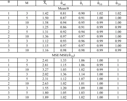
Table 1 shows the ratio of average value of the 500 estimates to the target θ and the ratio of their

empirical mean square error to that of ˆ θ _{2 0}. Not surprisingly, the sample mean is biased high. The weighted distribution esimator is biased low, the more so the greater the skewness (small θ,

large M). The downward bias can be confirmed theoretically; see the Appendix. It leads to

higher mean square error for the weighted distribution estimator than for the maximum

[image:14.595.67.505.133.483.2]

Table 1. Simulation results for array sampling of Poisson(θ) random variables (500

simulations with n = 20, ξ = 0.5)

θ _M X _{s θ} ˜

wd θ ˆ 1 θ ˆ 1 0 θ ˆ 2 0

Mean/θ

1 3 1.42 0.81 0.90 1.02 1.02

1 5 1.50 0.87 0.91 1.00 1.00

1 10 1.58 0.94 0.95 0.99 1.00

2 3 1.25 0.86 0.91 0.99 0.99

2 5 1.31 0.92 0.94 0.99 1.00

2 10 1.36 0.97 0.97 0.99 1.00

3 3 1.12 0.93 0.96 0.99 0.99

3 5 1.15 0.97 0.97 0.99 1.00

3 10 1.16 0.98 0.98 0.99 0.99

MSE/MSE(θ ˆ _{2 0})

1 3 2.41 1.33 1.06 1.00 1

1 5 2.81 1.15 1.06 0.99 1

1 10 3.27 1.03 1.02 0.99 1

2 3 2.02 1.36 1.14 1.00 1

2 5 2.31 1.12 1.07 1.00 1

2 10 2.63 1.02 1.01 1.00 1

3 3 1.55 1.20 1.09 1.00 1

3 5 1.80 1.05 1.03 1.00 1

3 10 1.89 1.02 1.02 1.00 1

In some circumstances therefore, the weighted distribution estimator may be a convenient

alternative to the maximum likelihood estimator. However, a general delineation of these

circumstances is an open question. The following artificial example illustrates that it is not just a

question of large M.

Example 3. Consider the estimating equation for a population of M normal random variables

with variance known (or one could consider a simple random sample)

X_j− µ

(

)

j=1 M

∑

=0 ,

X_i+ X_j

j≠i

∑

=Mµ.

Approximating the second term on left by (M-1)µ (as in (8)) gives the “approximate”

estimating equation

X_i+

(

M−1

)

µ =Mµ

yielding the estimator µ =ˆ X_i, which, although unbiased, is considerably less efficient than

ˆ

µ =X .

4.

A Generalisation to Unbiased Estimating Equations for the

Population Mean under Array Sampling

Consider estimation of the population mean µ of X under array sampling. Given the expression

(2) for the sample density of X, it is straightforward to show

E X

( )

_is =ME X ξ +X Mξ +X+U

⎧ ⎨ ⎩

⎫ ⎬ ⎭ ⎛

⎝

⎜ ⎞

⎠ ⎟

where X and U are independent and U is the sum of M-1 independent and identically distributed

realisations of X. Hence an unbiased sample-based estimating equation for µ is

X_is−ME X ξ +X

Nξ +X+U

⎧ ⎨ ⎩

⎫ ⎬ ⎭ ⎛

⎝

⎜ ⎞

⎠ ⎟ ⎧

⎨ ⎩

⎫ ⎬ ⎭ =0

i=1 n

∑

. (10)

Given a model for the population distribution of X (which will depend on the unknown

parameter θ), this equation can be solved for θ, and hence for µ = µ(θ), by Monte Carlo

simulation of the independent random variables X and U.

A generalisation of the MIP-based approach to estimation of µ is based on the following

unbiased population-based estimating equation for this parameter:

L(µ)=

(

X_ij− µ

)

j=1 M

∑

i=1 n

Let U_ir denote the sum of the nonsampled X-values in the it h row of the population. The MIP-based approach replaces the preceding estimating equation by

L_s(µ)=E L(

(

µ) sample data

)

=

{

(

X_is−µ

)

+E U

(

_ir −(M−1)µ X_is,A_i

)

}

i=1

n

∑

= X_is+(M−1)

E X

Mξ +X_is+U

⎛ ⎝

⎜ ⎞

⎠ ⎟

E 1

Mξ +X_is+U

⎛ ⎝

⎜ ⎞

⎠ ⎟ ⎧

⎨ ⎪ ⎪

⎩ ⎪ ⎪

⎫

⎬ ⎪ ⎪

⎭ ⎪ ⎪

i=1 n

∑

−Mnµ

= 0 (11)

where the third step follows from (5) with ∂_θlogf(X_ir) replaced with U_ir. This equation can be solved using Monte Carlo simulation of the independent random variables X and V, with U = X

+ V. Note that since L(µ) coincides with the ML estimating equation under a Poisson model, the

solution to (11) is the MIP estimate of µ = θ and will be the same as the expression for the

sample-based MLE of θ derived in Example 2.

The estimator of µ defined by the solution of (11) is consistent provided E(L_s(µ)) = 0. This follows directly from the fact that since L(µ) is an unbiased estimating equation,

E L

(

_s(µ)

)

=E E L(

(

(

µ) sample data

)

)

=E L(

(

µ)

)

=0 .

That is, a generalised MIP approach based on an unbiased population level estimating equation

for µ also leads to an unbiased estimating equation for this parameter.

5.

Extensions

An immediate (and straightforward) extension of the theory developed in the preceding sections

is to “ragged array sampling” where the it h “row” of the population array is of size M_i, i = 1, .., n. Of more interest, perhaps, is an extension to alternative methods of sampling within each

“row”, and in particular to cases where we are unsure whether the sampling method is

informative or not. One way of modelling this situation (within the array sampling framework) is

guess” about the probability that unit j in row i is selected, given the “characteristics” of the

units in row i. However, there is the chance that these ξ_{i j} do not “capture” the true probability of selection, which may in fact be related to the actual X-values in the row. We can model this

scenario by a straightforward extension of the array sampling probability model (1):

pr A

(

i = j ξik,Xik;k =1,2,L,Mi

)

=

ξij+ γXij

T_i(ξ)+ γT_i(X). (12)

Here γ is an unknown nonnegative parameter measuring the extent of “informativeness” of the

sampling method, T_i(ξ) is the total of the ξ_{i j} in row i and T_i(X) is the corresponding X-total. Exactly the same argument as that leading to (2) can then be used to show that the sample

density for X for a “draw” from row i of the population is

f_is(x)=f(x) T

(

_i(ξ)+ γM_ix

)

E 1

T_i(ξ)+ γ(x+U_i)

⎛ ⎝

⎜ ⎞

⎠

⎟ (13)

where U_i denotes the random variable corresponding to the sum of M_i-1 independent realisations of X. Independence of draws from different rows implies the score function for

θ and γ is then defined by the component score functions

sc_s(θ)= ∂θf(Xis) f(X_is) +

∂θE

1

T_i(ξ)+ γ(X_is+U_i)

⎛ ⎝ ⎜ ⎞ ⎠ ⎟ E 1

T_i(ξ)+ γ(X_is+U_i)

⎛ ⎝ ⎜ ⎞ ⎠ ⎟ ⎧ ⎨ ⎪ ⎪ ⎩ ⎪ ⎪ ⎫ ⎬ ⎪ ⎪ ⎭ ⎪ ⎪

i=1 n

∑

. (14)

and

sc_s(γ)= γ + ξ i X_is ⎛ ⎝ ⎜ ⎞ ⎠ ⎟ −1 + ∂γE

1

T_i(ξ)+ γ(X_is+U_i)

⎛ ⎝ ⎜ ⎞ ⎠ ⎟ E 1

T_i(ξ)+ γ(X_is+U_i)

⎛ ⎝ ⎜ ⎞ ⎠ ⎟ ⎧ ⎨ ⎪ ⎪ ⎩ ⎪ ⎪ ⎫ ⎬ ⎪ ⎪ ⎭ ⎪ ⎪

i=1 n

∑

. (15)

where ξ _i is the average of the ξ_{i j} in row i.

In theory, equations (14) and (15) can be solved numerically to get the MLE’s for θ and γ,

using, for example, Monte Carlo simulation and numerical differentiation to evaluate the second

provide insight into the sensitivity of the MLE for θ to the extent of “informativeness” in the

sample design.

Another relatively straightforward extension of array sampling is where the distribution of X

varies from one row of the array to the next. Of course, if one is interested in a parameter θ

which characterises the “overall” distribution of X, then a link between the “row specific”

distributions of X and its overall distribution has to be established before likelihood inference

about θ is possible. An example is where the rows are defined in terms of another variable Z

which is correlated with X. This seems a reasonable way of modelling ordered systematic

sampling, for instance, where the ordering is in terms of the values of Z.

The other major extension of the preceding theory is to situations where sample selection is not

draw by draw, as in array sampling, but where the entire sample is selected without replacement

at one draw. This situation can be modelled by a generalisation of (12). As usual we assume a

population of N independent and identically distributed realisations of a non-negative random

variable X, with a fixed sample size n drawn without replacement from this population. Let S

denote the set of all C_N,n = N![(N-n)!n!]-1 possible realisations of the sample label set s. We suppose that for each s in S we know a non-negative value ξ(s) such that the probability p(s) of

selection of the sample label set s given the population values of X can be modelled as

p(s)= ξ(s)+ γT(s)

ξ(t)+ γT(t)

{

}

t∈S

∑

(16)

where T(s) denotes the total of the X values for the population units in s. When γ > 0 (16)

corresponds to single draw informative sampling. Let K denote the total over S of ξ(s) and let T

denote the population total of X. Then (16) can equivalently be written

Let x denote a point in n-dimensional Euclidean space. Using the same argument as that leading

to (2) we can show that the joint density of the sample X-values at x under the sampling scheme

defined by (16) is

f_s(x)= f(x_i)

i=1 n

∏

E ξ(s)+ γΣ(x) K+ γ[Σ(x)+U]C_N−1,n−1 ⎡

⎣ ⎢

⎤ ⎦ ⎥

s∈S

∑

= f(x_i)

i=1 n

∏

[

K+ γΣ(x)C_N−1,n−1

]

E 1

K+ γ[Σ(x)+U]C_N−1,n−1 ⎡

⎣ ⎢

⎤ ⎦ ⎥

=

f(x_i)

i=1 n

∏

N K

[

+ γΣ(x)

]

E 1

K N+ γ[Σ(x)+U]n ⎡

⎣ ⎢

⎤

⎦ ⎥ . (17)

Here K is the average value of ξ(s) over all C_N,n samples in S, Σ(x) denotes the summation of the values in x and U is the sum of N – n independent and identically distributed realisations of

X.

Maximum likelihood inference for a parameter θ of the marginal distribution of X follows

directly from (17). Note that it is straightforward to combine this one draw sampling procedure

with the array sampling concept to provide a very general model for informative sampling. For

example, stratified informative sampling occurs where each row in the array is a stratum, and

Acknowledgements

This research was supported in part by the Texas Adanced Research Program

(010366-0286-1999), the National Cancer Institute (CA 57030) and the Texas A&M Center of Environmental

and Rural Health through a grant from the National Institute of Environmental Health Sciences

(P30-E509106).

References

Breckling, J. U., Chambers, R. L., Dorfman, A. H., Tam, S. M. and Welsh, A. H. (1994).

Maximum likelihood inference from sample survey data. International Statistical Review, 62,

349-363.

Chambers, R. L., Dorfman, A. H. and Wang, S. (1998). Limited information likelihood analysis

of survey data. Journal of the Royal Statistical SocietyB, 397 - 411.

Krieger, A. B. and Pfeffermann, D. (1992). Maximum likelihood estimation from complex

sample surveys. Survey Methodology, 18, 225-239.

Orchard, T. and Woodbury, M. A. (1972). A missing information principle: theory and

application. Proc. 6th Berkeley Symp. Math. Statist., 1, 697 - 715.

Rao, J. N. K., Hartley, H. O. and Cochran, W. G. (1962). On a simple procedure of unequal

probability sampling without replacement. Journal of the Royal Statistical Society B, 24,

Appendix: Weighted Distribution Estimator Bias in the Poisson Case

Under array sampling, the score function for the Poisson case can be written

sc_s

( )

θ =nM

θ

1

n E

1 a_i+B

⎧ ⎨ ⎩ ⎫ ⎬ ⎭ ⎛ ⎝ ⎜ ⎞ ⎠ ⎟

i=1 n

∑

−1− α

⎡ ⎣ ⎢ ⎢ ⎤ ⎦ ⎥ ⎥ ,

where α = ξ + θ, a_i = α + (X_{i s}−θ)/M, B = M-1[U-(M-1)θ], and the expectation operator conditions on the given value of X_{i s}. We shall assume α > θ > 1. Noting that

E 1

a_i+B

⎛ ⎝

⎜ ⎞ ⎠ ⎟ =E 1

a_i 1− B a_i +

B2 a_i2 −

B3 a_i3 +

B4 a_i4

⎛ ⎝ ⎜ ⎞ ⎠ ⎟ ⎡ ⎣ ⎢ ⎤ ⎦

⎥ +O_p 1 M3

⎛ ⎝ ⎜ ⎞ _⎠ ⎟

= 1

a_i 1+ M−1

(

)

θ

a_i2M2 − θa_i3M2 + 3θ2 a_i4M2

⎡ ⎣

⎢ ⎤

⎦

⎥ +O_p 1 M3

⎛ ⎝ ⎜ ⎞ _⎠ ⎟

we then have

sc_s

( )

θ =nM

θ

1 n _i=1ai

n

∑

1−

(

M−1

)

θ

a_i2M2 + θa_i3M2 − 3θ2 a_i4M2 + θ

2

a_i4M2

⎛ ⎝

⎜ ⎞

⎠

⎟ +O_p 1 M3

⎛ ⎝

⎜ ⎞ _⎠ ⎟ − α ⎡ ⎣ ⎢ ⎤ ⎦ ⎥ =nM θ

X _s− θ

M −

(M−1)θ M2

1 n

1 a_i i=1

n

∑

⎛ ⎝ ⎜ ⎞ ⎠ ⎟ + θ

M2 1 n

1 a_i2 i=1

n

∑

⎛ ⎝ ⎜ ⎞ ⎠ ⎟ −2θ

2

M2 1 n

1 a_i3 i=1

n

∑

⎛ ⎝ ⎜ ⎞ ⎠ ⎟ ⎛ ⎝

⎜ ⎜ ⎞ _⎠ ⎟ ⎟ +O_p 1 M3 ⎛ ⎝ ⎜ ⎞ _⎠ ⎟ ⎡ ⎣ ⎢ ⎢ ⎤ ⎦ ⎥ ⎥ =n

θ X s− θ − θ_{θ + ξ}+ θ 1 α − 1 n 1 a_i i=1

n

∑

⎛ ⎝ ⎜ ⎞ ⎠ ⎟ + θ

n 1 a_i i=1

n

∑

+ θ

n 1 a_i2 i=1

n

∑

−2θ2

n 1 a_i3 i=1

n

∑

⎛ ⎝ ⎜ ⎞ ⎠ ⎟ 1

M+Op 1 M2 ⎛ ⎝ ⎜ ⎞ _⎠ ⎟ ⎡ ⎣ ⎢ ⎤ ⎦ ⎥

≈sc_wd

( )

θ + n Mθ

θ

(

X _s− θ

)

α2 + θ_α+ θ_α2 − 2θ2

α3 ⎛ ⎝ ⎜ ⎞ ⎠ ⎟ ⎡ ⎣ ⎢ ⎢ ⎤ ⎦ ⎥ ⎥

>sc_wd

( )

θ + n M

X _s− θ

(

)

α2

for α > 1, since then θ/α > θ2/α3 and θ/α2 > θ2/α3. Moreover, under array sampling

E X

(

s − θ

)

>0. Thus, asymptotically,

E sc

(

_wd(θ)

)

<E sc

(

_s(θ)

)

−nE(X s)− θ

Mα2 = −n

E(X _s)− θ Mα2 <0 .