Large eddy simulation of transonic turbulent flow over a bump

Large-eddy simulation of transonic turbulent flow over a bump

N.D. Sandham

, Y.F. Yao

, A.A. Lawal

a_{Aerodynamics & Flight Mechanics Research Group, School of Engineering Sciences, University of Southampton, Southampton SO171BJ, UK}

b_{Alstom Power UK Ltd., P.O. Box 1, Waterside South, Lincoln LN5 7FD, UK}

Received 23 November 2002; accepted 5 March 2003

Abstract

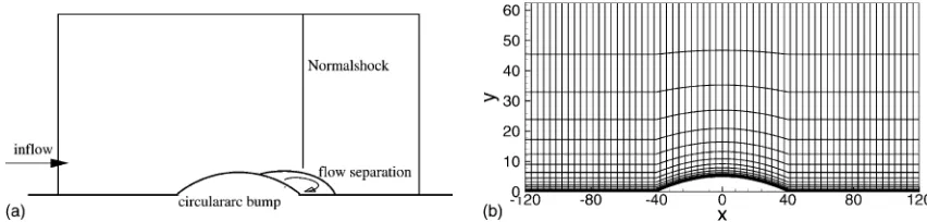
Transonic turbulent boundary-layer flow over a circular-arc bump has been computed by high-resolution large-eddy simulation of the compressible Navier–Stokes equations. The inflow turbulence was prescribed using a new technique, in which known dy-namical features of the inner and outer part of the boundary-layer were exploited to produce a standard turbulent boundary-layer within a short distance of the inflow. This method was separately tested for a flat plate turbulent boundary-layer, for which results compared well with direct numerical simulation databases. Simulation of the bump flow was carried out using high-order methods, with the dynamic Smagorinsky model used for sub-grid terms in the momentum and energy equations. Simulations were carried out at a Reynolds number of 233,000 based on bump length and free-stream properties upstream of the bump. At a back pressure equal to 0.65 times the stagnation pressure, a normal shock was formed near the bump trailing-edge and a peak mean Mach number of 1.16 was observed. Turbulence fluctuations decayed in the favourable pressure gradient region of the flow, before being amplified due to the shock interaction and boundary-layer separation. The effect of Reynolds number on turbulence intensity upstream of the shock is discussed in connection with a laminarisation parameter. With reference to turbulence modelling, anisotropy levels are not unreasonably high in the shock interaction region and shock unsteadiness was not found to be an issue. Of more relevance to the perceived poor performance of models for this type of flow may be the extremely rapid rise and decay of turbulence levels in the separated shear layer immediately under the shock-wave.

Ó2003 Elsevier Science Inc. All rights reserved.

Keywords:Direct numerical simulation; Large-eddy simulation; Compressible turbulence; Shock/boundary-layer interaction

1. Introduction

Shock/boundary-layer interaction (SBLI) phenomena have important applications in a wide range of practical problems, such as transonic airfoils and wings, super-sonic engine intakes, diffusers of centrifugal compres-sors, and turbo-machinery cascades. Pioneering research into SBLI was carried out by Liepmann (1946), who did the earliest experiments on laminar and turbulent boundary-layers interacting with a normal shock-wave. Since then considerable progress has been made towards understanding the complex interaction mechanisms. A review by Green (1970) summarized three major inter-action scenarios: (i) a sharp compression corner gener-ating an outgoing oblique shock-wave, (ii) the reflection

of an incident oblique shock at a plane wall, and (iii) a weak normal shock-wave interacting with a spatially-developing boundary-layer, in which there is no curva-ture effect. For many practical flows, the interaction takes place at transonic speed on a curved surface, where the turbulent boundary-layer experiences large

pressure gradients. Experimental investigations of

shock/turbulent-boundary-layer interaction with non-zero pressure gradients have been carried out by Delery (1983) using a variable-curvature bump geometry, and by Liu and Squire (1988) using a circular-arc bump geometry. Both studies showed significant flow changes in the transonic regime, including ak-shock pattern and extensive flow separation. Various techniques were used in the experiments in order to establish the details of both the mean flow and the turbulence. An additional study was made by Liu and Squire (1988) into the effect of curvature, using models of different radius and dis-tinguishing between shock-induced separation and

*

Corresponding author. Tel.: 4872; fax: +44-23-8059-3058.

E-mail address:[email protected](N.D. Sandham).

0142-727X/03/$ - see front matterÓ2003 Elsevier Science Inc. All rights reserved. doi:10.1016/S0142-727X(03)00052-3

bump trailing-edge separation (due to the adverse pressure gradient, independent of the shock).

With advances in computer technology and the development of suitable numerical algorithms, compu-tation of SBLI has become feasible. The Reynolds-averaged Navier–Stokes (RANS) approach has been widely used and direct numerical simulation (DNS), with the advantages of resolving all scales of fluid mo-tions, has also been adopted for the study of several model problems. Although DNS is limited to low Rey-nolds numbers and simple geometries, it offers a com-plete reference for the given flow, which is invaluable for understanding flow physics and assessing turbulence models. Adams (2000) carried out a direct simulation of turbulent boundary-layer flow over a compression

cor-ner at Mach number 3 and Reynolds number Re_h¼

1685 (based on the inflow momentum thickness). A

deflection angle of b¼18° was chosen to generate a

small (but more than incipient) flow separation, and a database was produced for model assessment. Numeri-cal studies of an incident oblique shock-wave interacting with a two-dimensional laminar boundary-layer have been carried out by Katzer (1989) and Wasistho (1998). Further 3D studies are needed for strong interactions where the flow exhibits significant three-dimensionality and unsteady behaviour. Channel flow with the Delery (1983) bump geometry has been studied in some detail by RANS, for example Loyau et al. (1998) using a non-linear eddy-viscosity model and Batten et al. (1999) using a full Reynolds stress model. Unsatisfactory pre-dictions of flows with significant SBLI is attributed to various deficiencies in the models, such as a failure to resolve anisotropy of the normal stresses. It is also a concern that steady state solvers will be in error if the flow is naturally unsteady and the shock location oscil-lates. Large-eddy simulation (LES) has not been widely applied to shock/boundary-layer interaction problems. Stolz et al. (2001) have demonstrated the potential for this approach using an approximate deconvolution

sub-grid model to obtain good comparisons with AdamsÕ

ramp flow DNS. Also Garnier et al. (2002) used LES to simulate shock impingement onto a turbulent boundary-layer at Mach 2.3. No simulations of the fully turbulent transonic bump flow problem have been published to date.

Recently Lawal and Sandham (2001) demonstrated the feasibility of a DNS approach for boundary-layer flow over the Delery bump with shock/laminar-boundary-layer interactions and flow transition to turbulence. In that study the upstream boundary-layer was laminar with transition triggered by a disturbance strip at the crest of the bump. The object of the present study is to extend the DNS/LES capability to turbulent boundary-layer flow over a bump geometry at tran-sonic speed with turbulent shock/boundary-layer in-teractions.

2. Simulations

Both direct and large-eddy simulations have been run for this investigation. Key features of the code are de-scribed in this section together with details of the flow configuration chosen for study.

2.1. Governing equations and numerical method

We consider the motion of a Newtonian fluid, which is governed by the fundamental conservation laws for mass, momentum, and energy. In the following, we use an asterisk to denote dimensional quantities and a subscriptÔ0Õto denote stagnation quantities. Stagnation properties are a convenient reference for this flow since experiments are typically run by exhausting from an upstream reservoir of effectively stationary fluid. A thermally perfect gas with constant specific heat capa-cities (cpat constant pressure andcvat constant volume)

is assumed and the ratioc¼cp=cvis set to be 1.4. The

non-dimensional viscosity l (referenced to its value at the stagnation temperature) is assumed to satisfy the

power law l¼TX, where T is the non-dimensional

temperature referenced to stagnation temperature with X¼0:76. For convenience, tensor notation is used with subscripts 1, 2 and 3 representing the streamwise (x), wall-normal (y) and spanwise (z) coordinates respec-tively. Non-dimensionalization is carried out by

q¼q_=q

0; ui¼ui=a0; p¼p=ðq0a 2 0 Þ;

T ¼T=T₀; E¼E=ðq 0a

2 0Þ:

Here, the termsq,ui,p andE denote the density, three Cartesian velocity components, the pressure and the total energy (E¼p=ðc1Þ þquiui=2), while a0 is the dimensional stagnation sound speed. Time is non-dimensionalized by d₁=a

0, where d

1 is the dimensional inflow boundary-layer displacement thickness. The Reynolds number specified in the bump flow simulations is defined by Re0¼q0a0d

1=l0¼5197. For reasons of comparison with experiment we will also quote the

Reynolds number based on d1 and upstream flow

properties, which isRe¼2910.

The compressible Navier–Stokes equations can be written in a compact notation as

oU

ot þ

oFI

ox þ

oGI

oy þ

oHI

oz ¼

oFV

ox þ

oGV

oy þ

oHV

oz ; ð1Þ

where the conservative variables are U ¼ ½q;qui;E T

. The convective and diffusive fluxes are FI_{, G}I_{, H}I _and

The principal issue in shock-wave/turbulence simu-lations is that good numerical methods for turbulence are generally inefficient for shock flows, while the best shock-capturing schemes are much too dissipative for accurate resolution of turbulence. Three main tech-niques are commonly used in shock–turbulence simu-lations: full shock resolution, essentially non-oscillatory (ENO) schemes, and hybrid methods, in which the method varies depending upon whether a shock-wave is detected. The former two methods have proved too ex-pensive for routine calculations and consequently hybrid methods have most commonly been used. Recently a stable numerical method applying the concept of en-tropy splitting has been developed, in which 4th- or 6th-order (compact or non-compact) central differences were implemented together with a total variation diminishing (TVD) scheme with the artificial compression method (ACM) for detecting the shock-wave. In addition, a stable high-order numerical boundary treatment was used based on the summation by parts (SBP) approach of Carpenter et al. (1999). The idea of entropy splitting is to split the inviscid flux derivatives into a conservative part and a symmetric part based on an entropy variable. Experience shows that such a splitting procedure im-proves the non-linear stability and minimizes the nu-merical dissipation for both smooth flows and for problems with complex shock–turbulence interactions. The entropy splitting procedure was applied to the Euler terms given on the left hand side of Eq. (1) and details of the formulation can be found in Sandham et al. (2002). The shock-capturing algorithm is described in Yee et al. (1999).

Two numerical parameters are associated with the method and must be set for each simulation. A splitting

parameter b fixes the proportions of conservative and

symmetric formulations of the Euler terms. Enhanced non-linear stability is typically found for 1:25<b<12

(Sandham et al., 2002), and we take b¼4 for

simula-tions presented here. A shock-capturing parameter j

also needs to be specified. Despite the success of the ACM method in localising the effect of the extra dissi-pation to the immediate vicinity of the shock-wave, it is still advisable to keep j as small as possible, without incurring oscillations near shock-waves. For mixing layer and shock tube problems we have typically em-ployedj¼0:7 (Yee et al., 1999; Lawal, 2002). For the current work we setj¼0 for the shock-free turbulent

boundary-layer andj¼0:2 for the bump flow LES.

The simulation uses a parallel compressible LES/ DNS code developed by Yao et al. (2000), which em-ploys 4th-order central finite differences for spatial

de-rivatives and a 3rd-order explicit Runge–Kutta

algorithm for time advancement. Generalized coordi-nates are used so that complex geometries can be trea-ted. Validations of the code have included vortex merging by Yee et al. (1999), shock tube flows by Lawal

(2002), turbulent channel flow by Sandham et al. (2002) and supersonic turbulent boundary-layer flow by Li (2003).

For large-eddy simulation we consider the filtered Navier–Stokes equations, which contain extra terms that must be modelled, in particular the stress term

q

qsij ¼quiujquiquj=qq ð2Þ

appears in both the momentum and energy equations. With the dynamic Smagorinsky model of Germano et al. (1991) the stress term is modelled by

sij¼CdD2jSjSij ð3Þ

where Cd is a constant, to be defined dynamically,Dis a filter width, and Sij is the strain rate deduced from the density-weighted velocity field uu~i¼qui=qq. In com-mon with many other LES of wall-bounded turbulence we do not do any filtering in the wall-normal direction. The Lilly (1992) least-squares method of determining the constant is used. A top-hat filter with trapezoid integration is applied in physical space as the test filter of the dynamical procedure. This filter has width D¼2h, where h is the grid spacing. In this case we have one homogeneous direction, so averaging is taken over that direction. Any negative values of the Sma-gorinsky constantCddetermined by this method are set to zero.

There are additional sub-grid terms in the energy equation (Vreman (1995) gives a complete list). At the low Mach numbers of transonic flow (peak Mach numbers 1.2, peak convective Mach number 0.6) it is unlikely that these will be significant. Nevertheless we include a modelling of these terms via an additional heat flux, which under our normalisation can be written as

qt_i¼CdqqD

2_jSj

Prtðc1Þ

oT

oxi

ð4Þ

where the turbulent Prandtl number Prt is set to unity.

2.2. Problem definition

The inflow mean turbulent boundary-layer

displace-ment thickness d₁ is taken equal to 1/5 of the bump

height. The factor of 1/5 is chosen so that dimensionless distances in the simulation correspond numerically to dimensions in millimetres in the Liu and Squire (1988)

experiments. The computational domain is then

24062.516 in the streamwise, wall-normal and

spanwise directions respectively. The solution is as-sumed to be periodic in the spanwise direction. The circular-arc bump, which has a length of 80, a height of 5 and a radius of 163 (all based ond₁), is located in the middle of the lower surface. The length of the up- and downstream flat plate is taken as 80. Grid points are uniformly distributed in the streamwise and spanwise directions and stretched in the wall-normal direction with more points clustered in the near-wall region. Fig. 1(b) shows a side-view of the computational domain.

The optimum choice of Reynolds number for the simulations turned out to be quite involved. Early work, as presented in Yao and Sandham (2002) used DNS at

Re¼1000 based on incoming boundary-layer

displace-ment thicknessd₁ and free-stream flow conditions. For shock locations near the end of the bump, comparable to the Liu and Squire (1988) experiments, it was found that only slightly supersonic peak Mach numbers

Mp¼1:05 were obtained. Additionally, at this Reynolds

number, there was a partial laminarisation of the flow near the top of the bump, leading to early separation of the boundary-layer. There was still sufficient turbulence in the flow to give a closed separation bubble compa-rable in length to that observed in experiments, however this was found to be sensitive to the upstream forcing. Despite flow phenomena involving laminarisation and re-transition being of considerable interest, it was de-cided additionally to attempt an LES at a higher Rey-nolds number (nominally 3000, in practice 2910 as the inflow velocity adjusts according to the back pressure). Results from this simulation, presented in this paper, are expected to be more representative of fully turbulent bump flow, despite the additional modelling errors in-troduced by moving from a DNS to an LES approach. The issue of laminarisation is discussed further in Sec-tion 4.3. The Reynolds number of 2910 based on inflow displacement thickness and free-stream conditions

cor-responds toRe0¼5197 with reference velocity taken as

the stagnation sound speed. A Reynolds number based on bump length and free-stream properties is 233,000. This is still well below the original Liu and Squire (1988) experiments, where a comparable Reynolds number was

1.6106, but does allow high-resolution LES to be

made.

2.3. Boundary conditions

A proper description of turbulent inflow conditions is always a challenge for DNS. Previous studies, for example the compressible ramp flow (Adams, 2000) and the incompressible trailing-edge flow (Yao et al., 2001), used an additional precursor simulation to de-fine the turbulent inflow. The method works well but at extra cost in CPU time, data storage and simulation complexity. In this simulation a new approach is used to prescribe the turbulent inflow, in which known dy-namical features of the inner and outer part of the boundary-layer are reproduced, including liftedÔstreaksÕ and coherent outer-layer motions, superimposed with random noise to break remaining symmetries. The method has first been tested for a zero-pressure-gradient turbulent boundary-layer and then used in the bump simulation.

At the subsonic inflow, the velocity is initially ex-trapolated from the interior. The computed total mass flow rate is then used in combination with the analytic turbulent mean velocity profile of Spalding (1961) (at

the nominal Reynolds number Re¼3000) to give a

complete inflow profile. Pressure and density in the free stream are computed by assuming isentropic flow from a reservoir to the inflow (Lawal, 2002). Fluctuations were introduced using the method described in the next sec-tion. At the subsonic outflow, the derivatives of density and three velocity components were assumed to be zero and a fixed back pressure was prescribed. At the lower wall, a no-slip condition was used for the velocity components and an isothermal wall condition was pre-scribed with a temperature equal to the stagnation temperature. At the upper surface, a free-slip boundary condition was applied. Periodic boundary conditions were used in the spanwise direction.

3. Turbulent boundary-layer flow

Simulation of a compressible turbulent boundary-layer at Mach number 0.6 and Reynolds number

Re¼1000 (based ond₁ and the free-stream quantities) was carried out to validate a new method for prescribing turbulent inflow conditions. It is well understood that the inner layer of the turbulent boundary-layer has low speed streaks, which at high amplitude become unstable, while the outer layer has large scale coherent structures. In order to reproduce turbulent flow numerically, a fixed spectrum is commonly used. This method omits phase information and consequently it takes a long distance from the inflow to fully develop the turbulence. Here we follow a more deterministic approach and introduce specific inner- and outer-layer disturbances, with asso-ciated phase information. Disturbances in the inner re-gion (denoted as uu^inner_{) are used to represent lifted}

streaks, with a peak at a location ofy_p;jþ, while the outer-region disturbances (denoted as uu^outer_{) represent}

three-dimensional vortices. The disturbances take the form:

^

u

uinner ¼c1;0yþe yþ_=yþ

p;0_sinð_x

0tÞcosðb0zþ/0Þ ð5Þ

^

vvinner ¼c2;0ðyþÞ2eðy þ_=yþ

p;0Þ 2

sinðx0tÞcosðb0zþ/0Þ ð6Þ

^

u

uouter¼X

3

j¼1

c1;jy=yp;jey=yp;jsinðxjtÞcosðbjzþ/jÞ ð7Þ

^

vvouter¼X

3

j¼1

c2;jðy=yp;jÞ 2

eðy=yp;jÞ2_sinðx

jtÞcosðbjzþ/jÞ

ð8Þ

where subscriptsj¼0, 1, 2, 3 are mode indices,yþ_{is the}

y-coordinate in wall units defined asyþ_¼q

wyus=lw and theci;jare constants. Forcing frequencies are denoted by xj, spanwise wave numbers by bj, and phase shifts by /j. The spanwise velocity w is derived from a diver-gence-free condition, since we do not expect dilatational compressibility effects to appear until much higher Mach numbers than are studied here. Density and temperature fluctuations are expected to develop natu-rally once the turbulent velocity field is established.

For inner-layer disturbances, the characteristic fre-quencyxjis estimated by assuming that the disturbance

travels downstream for a distance of kþ_x ’500p at a

convective velocity Uc’10us within a complete time

period (low speed plus high-speed streak), while the wave number bj is derived by assuming a typical

char-acteristic spanwise streak spacing of kþz ¼100. For

outer-layer disturbances, the characteristic frequencyxj

is estimated by assuming that the disturbance travels downstream for a distance of kx’16 at a velocity of

about 0:75U1 within a complete time period. The wave

numbers bj are chosen to give a range of outer-layer

structures with a scale up to the computational box size. Table 1 gives a summary of the parameters used in the demonstration flat plate boundary-layer simulation. The streamwise and wall-normal fluctuations were generated with one mode in the inner region and three modes in the outer region. Additional random noise with a max-imum amplitude 4% of the free-stream velocity was used to break any remaining symmetries in the inflow con-dition.

To test the method, a computational domain of

50108 was used with a grid of 1929664 points,

uniformly distributed in the streamwise and spanwise directions and stretched in the wall-normal direction. The grid resolutions, estimated based on the inflow quantities, are Dxþ¼13:0, Dzþ¼6:25 and the first point is at about yþ¼0:92 with a total of 10 points in

the viscous sub-layer up to yþ¼10. The simulation

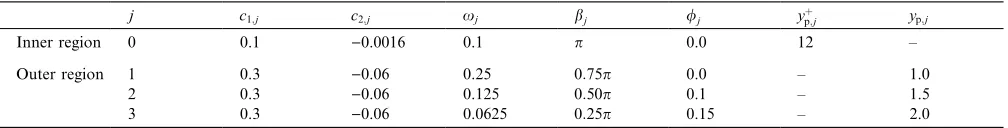
starts with a uniform flow field equal to the mean pro-files of the inflow turbulence. The inflow turbulence fluctuations were introduced as described above. The simulation was initially run for 100 time units and sta-tistical samples were accumulated for a further 100 time units, with a total of 4600 samples, using 32 processing elements (PEÕs) on an SGI Origin 3000 system. Fig. 2(a) shows a comparison of the simulated mean velocity profile with the law of wall and the incompressible DNS of Spalart (1988). Fig. 2(b) shows the turbulence inten-sities and Reynolds stress distributions using the defect

coordinate (g), which compare well with the Spalart

DNS data. Compressibility effects are not expected to be significant for this attached-flow simulation at Mach number 0.6. Improved comparisons are of course ob-tained if one moves further downstream, however the results shown here, obtained only 40d₁ from the inflow, are already adequate for our purposes. A suitable tur-bulent boundary-layer has been obtained far sooner with this method than if one had started with laminar

Table 1

Parameters for inflow turbulent fluctuations for the turbulent boundary-layer test case

j c1;j c2;j xj bj /j ypþ;j yp;j

Inner region 0 0.1 ₎0.0016 0.1 p 0.0 12 –

Outer region 1 0.3 ₎0.06 0.25 0:75p 0.0 – 1.0

2 0.3 ₎0.06 0.125 0:50p 0.1 – 1.5

flow and forced transition via a time-varying wall-transpiration condition. The method has been extended to boundary-layer flow at Mach 2 by Li (2003).

4. Turbulent flow over a circular-arc bump

The large-eddy simulation of bump flow uses a

computational domain of 24062.516 with a grid of

54116161 points, uniformly distributed in the

streamwise and spanwise directions and stretched (with a grid expansion factor of 1.035) in the wall-normal di-rection. At inflow the grid resolution is approximately Dxþ¼32, Dzþ¼17 with 15 points in the viscous sub-layer (yþ<10). Such a grid resolution is quite good for LES, since we are within a factor of two of DNS-type resolutions in horizontal directions, and better than many DNS in the wall-normal direction. At the worst

location downstream where we have Dxþ¼49,

Dzþ¼28:5 with 9 points in the viscous sub-layer. For the channel flow test case used by Sandham et al. (2002) with the present code, good turbulence results were ob-tained at such resolutions without any sub-grid model.

The simulation uses a length ofLz¼16 in the periodic

spanwise direction. Based on the inflow mean 99.5% boundary-layer thicknessd0¼7:7, the ratio of Lz=d0 is

about 2.1, larger than the ratio of 1.22 used in DNS of ramp flow by Adams (2000), for which a two-point correlation study was carried out. For the reference

in-flow condition of Reynolds number Re¼3000, the

spanwise length in wall units is aboutLþ_z ¼1721. Table 2 shows the forcing constants for this case. Compared to the flat plate boundary-layer some of the

constants were altered to account for the different boundary-layer Reynolds number and an extra outer-layer mode was added due to the spanwise box being chosen twice as wide as in the boundary-layer test case. A fixed back pressure, equal to 0.65 times the stag-nation pressure was prescribed. The simulation was then run for a time of 2800 (about 8 flow-through times) to set up the initial flow field and then statistical samples were accumulated for a further 1200 time units (3.3 flow-through times) with a total of 16,000 samples, using 128 PEÕs on an SGI Origin 3000 system.

4.1. Structure of the flow

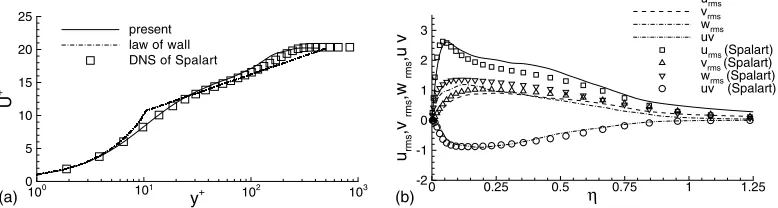
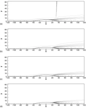
The instantaneous Mach number and pressure con-tours, shown in side-view on Fig. 3, illustrate that a

normal shock is formed at x¼32, close to the bump

trailing-edge atx¼40. The developing turbulence fluc-tuations have been weakened in the first-half of the bump due to the favourable pressure gradient, but then re-develop in the second-half of the bump where an adverse pressure gradient exists. The fluctuations are greatly amplified after the separation.

Fig. 4 shows contour plots of the time- and span-averagedM,p,qandT. Despite the averaging the shock is still crisply captured in these views, indicating that outside the boundary-layer the flow is steady and spanwise-independent. The pressure and density plots

show the beginnings of a k-shock structure, with the

front leg appearing as a weak Mach wave from just upstream of the separation point near x¼9. It should be noted how much the boundary-layer has thinned as it moves over the bump. At the top of the bump the 99%

Table 2

Parameters for inflow turbulent fluctuations in the bump simulation

j c1;j c2;j xj bj /j ypþ;j yp;j

Inner region 0 0.08 ₎0.0014 0.38 2p 0.0 12 –

Outer region 1 0.3 ₎0.06 0.125 0:25p 0.1 – 1.0

2 0.3 )0.06 0.0625 0:50p 0.2 – 1.5

3 0.3 )0.06 0.031 0:75p 0.3 – 2.0

4 0.3 )0.06 0.05 0:125p 0.4 – 1.5

y+

U

+

100 ₁₀1 ₁₀2 ₁₀3

0 5 10 15 20 25

present law of wall DNS of Spalart

η

urms

,v

rms

,w

rms

,u

v

0 0.25 0.5 0.75 1 1.25

-2 -1 0 1 2 3

urms

vrms

w_rms uv urms(Spalart)

v_rms(Spalart) wrms(Spalart)

uv (Spalart)

(a) (b)

thickness is only around 0.5 and can barely be discerned on these plots. The peak Mach number is 1.16, obtained atx¼32,y¼62:5.

The skin friction (Cf) distribution along the

streamwise direction, shown on Fig. 5(a), reveals many features of the flow. After a short transient where the skin friction recovers from the inflow condition it settles to a level around 0.0005. The influence of the

bump starts to be felt at x¼ 70 and after x¼ 60

the skin friction drops sharply, going negative in the short separation bubble at the leading edge of the bump. Note that this circular-arc bump does not have any smoothing at the transition to the flat plate (in contrast to the Delery (1983) bump geometry). The skin friction increases rapidly over the bump as the boundary-layer thins. From Fig. 4(c) the pressure

minimum is reached on the wall at x¼4 and

there-after a strong adverse pressure gradient serves to

sep-arate the boundary-layer at x¼9. The reattachment

occurs downstream at x¼50 with the skin friction

distribution in between quite typical of thin separation zones: an initial zone with small recirculation and barely negative skin friction, followed by a strong mean recirculation vortex above the largest negative values of skin friction. The skin friction relaxes downstream of the reattachment, reaching values of

0.006 by x¼100. The final rise at x¼120 is not

physical, but due to the fixed back pressure applied at the outflow boundary. Fig. 5(b) shows the wall pres-sure (normalised by stagnation prespres-sure) and Fig. 5(c) the free-stream Mach number distributions. The front part of the bubble is characterised by a plateau in the wall pressure. The pressure gradient downstream of the reattachment is mildly adverse initially, but then re-duces to zero. The mean Mach number increases from

0.72 at the inflow to 1.16 at the maximum at x¼32.

The largest streamwise gradient of the mean Mach number is seen near the crest of the bump. The pres-sure increase across the shock p2=p1¼1:40 is

consis-tent with the normal shock relation at M ¼1:16 (with an identical p2=p1¼1:40).

Although at a factor of nearly seven lower Reynolds number than the experiments of Liu and Squire (1988) it is worth making some quantitative comparisons. Com-pared to experiment the key difference is the location of separation. In the experiment, albeit with the shock in a slightly more rearward location, the separation is at

x’21. This is an eighth of a bump length behind the

LES with the consequence that in the experiment there is a greater turning angle of the flow at separation and consequently a stronger front leg of thekshock. Bubble lengths are about the same since the experimental reat-tachment is further back by about 10 x-units compared to the simulation. The simulated wall pressures closely match the experimental values upstream and along the first-half of the bump. In the second-half of the bump the experimental wall pressure decreases for a longer distance than in the simulations due to the delayed separation. The peak Mach number (Mp) of the

experi-ments is Mp’1:27, which is significantly higher than

seen in the simulations and a consequence of the later separation.

4.2. Turbulence statistics

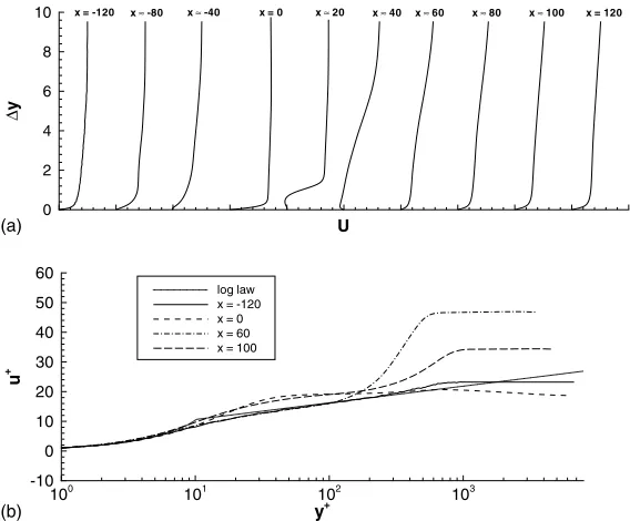
Fig. 6(a) shows the simulated mean velocity profiles at ten different downstream locations. Noteworthy fea-tures include the extreme thinning of the boundary-layer at the top of the bumpx¼0, the reverse flow (maximum magnitude around 16% of the local free stream) for x

y

-120 -100 -80 -60 -40 -20 0 20 40 60 80 100 120

0 10 20 30 40 50 60

x

y

-120 -100 -80 -60 -40 -20 0 20 40 60 80 100 120

0 10 20 30 40 50 60

(a)

(b)

20<x<40, and the recovery forx>60. Selected pro-files are plotted in wall unitsuþ_againstyþ _{on Fig. 6(b),}

compared with a standard law of the wall uþ_¼

2:44 logyþþ5:0. Due to the low Mach numbers it was not considered necessary to apply any van Driest-type normalisation. It can be seen that at the top of the bump the boundary-layer profile is reduced to a total thicknessdþ’60 with an edge velocityU_eþ’20. In the recovery region downstream of reattachment we see profiles that are changing quite rapidly, with a trend for

the large wake component to reduce. For exampleU_eþ

reduces from 47 atx¼60 to 34 atx¼100. The domain is not long enough to see complete relaxation to an equilibrium turbulent boundary-layer. For comparison the shape factor of the boundary-layer (with

integra-tions carried up to the point where the velocity profiles first reach 99% of the value on the upper boundary) is 1.49 at inflow, 1.36 at the top of the bump, 2.44 at

x¼60, reducing to 1.68 atx¼100.

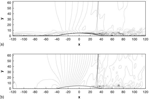
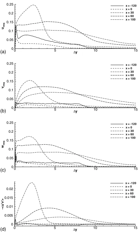
Contour plots of the root-mean-square (RMS) tur-bulence fluctuationsuRMSvRMSandwRMS are shown on

Fig. 7(a)–(c) with the Reynolds stresshu0v0ishown on Fig. 7(d). These plot are dominated by the behaviour of the turbulence downstream of separation and especially in the recirculation region. Peak values are seen at

x¼30 in the middle of the separated shear layer

im-mediately under the foot of the main shock-wave.

Pro-files of these turbulence quantities are shown at x

locations of)120, 0, 30, 60 and 100 on Fig. 8. The RMS turbulence quantities are reduced by a factor of about x

y

-120 -100 -80 -60 -40 -20 0 20 40 60 80 100 120

0 10 20 30 40 50 60

x

y

-120 -100 -80 -60 -40 -20 0 20 40 60 80 100 120

0 10 20 30 40 50 60

x

y

-120 -100 -80 -60 -40 -20 0 20 40 60 80 100 120

0 10 20 30 40 50 60

x

y

-120 -100 -80 -60 -40 -20 0 20 40 60 80 100 120

0 10 20 30 40 50 60

(a)

(b)

(c)

(d)

U

∆

y

0 2 4 6 8

10 x = -120 x≈-80 x≈-40 x = 0 x≈20 x≈40 x≈60 x≈80 x≈100 x = 120

y+

u

+

100

101

102

103

-10 0 10 20 30 40 50 60

log law x = -120 x = 0 x = 60 x = 100 (a)

(b)

Fig. 6. Mean velocity profiles (a) at differentx-locations and (b) in wall units.

x cf

-120 -100 -80 -60 -40 -20 0 20 40 60 80 100 120

-0.002 -0.001 0 0.001 0.002 0.003

cf= 0

x

M

-120 -100 -80 -60 -40 -20 0 20 40 60 80 100 120

0.6 0.7 0.8 0.9 1 1.1 1.2

x pw

/p0

-120 -100 -80 -60 -40 -20 0 20 40 60 80 100 120

0.3 0.4 0.5 0.6 0.7 0.8

(a)

(b)

(c)

Fig. 5. Streamwise (x) variation of (a) skin friction (wall shear stress normalised by 0:5q

0a20), (b) wall pressurepw=p0and (c) free-stream Mach

three relative to the inflow by the top of the bump, but then increase rapidly. At x¼60 after reattachment the RMS turbulence quantities are still four times inflow levels, reducing by a factor of two byx¼100.

A failure to model anisotropy of turbulence is a possible factor in the poor performance of turbulence models for SBLI problems. However here we do not see very extreme values. The ratio of peak values of

uRMS:vRMS:wRMS is 1.42:0.90:1 atx¼30, 1.21:0.95:1 at

x¼60 and 1.26:1.05:1 at x¼100. Obviously the

an-isotropy in the very near-wall region is much higher, but this is well known and does not prevent good predic-tions from models of equilibrium flat plate boundary-layer flows. Of more relevance to the perceived poor performance of models for this type of flow may be the extremely rapid rise and decay of turbulence levels in the separated shear layer immediately under the shock-wave.

4.3. Potential for laminarisation

A widely-used acceleration parameter that can be linked to laminarisation (see for example Jones and Launder, 1972) is

K ¼ le

qeUe2 dUe

dx ; ð9Þ

where a subscript edenotes free-stream properties, the criterion for laminarisation is roughly K>3106_, although this depends on the streamwise extent for which the favourable pressure gradient is sustained, and presumably also on the Reynolds number. The value of

K in our simulations depends on the wall-normal

loca-tion. If this is taken at the upper boundary of the simulation we haveKmax¼1:65106and if it is taken at a distanceDy¼20 above the surface we haveKmax¼ 2:35106_{. (The contribution from the wall-normal} x

y

-120 -100 -80 -60 -40 -20 0 20 40 60 80 100 120

0 10 20 30 40 50 60

x

y

-120 -100 -80 -60 -40 -20 0 20 40 60 80 100 120

0 10 20 30 40 50 60

x

y

-120 -100 -80 -60 -40 -20 0 20 40 60 80 100 120

0 10 20 30 40 50 60

x

y

-120 -100 -80 -60 -40 -20 0 20 40 60 80 100 120

0 10 20 30 40 50 60

(a)

(b)

(c)

(d)

Fig. 7. Contour plots of turbulence quantities (a)uRMS(max¼0.25, min¼0), (b)vRMS(max¼0.16, min¼0), (c)wRMS(max¼0.18, min¼0) and

component of velocity has been neglected for this cal-culation.) We conclude that laminarisation should not be an issue here. However, we can see that at the Rey-nolds numbers used for previous DNS calculations of Yao and Sandham (2002) the criteria would be exceeded locally, even if there is not a sufficient streamwise length of exposure to this level ofK to cause a complete lam-inarisation of the boundary-layer. It is concluded that the present simulations are just in excess of the mini-mum Reynolds number for fully turbulent bump flow. Full DNS of this case would require a factor of about four more grid points inx and z. Obviously this is ex-pensive, and our current thoughts are that DNS studies of fully turbulent SBLI are probably better focused on ramp and shock impingement test cases. The current case remains a good case for comparative testing of sub-grid models and numerical parameters in LES at lower resolutions, since it contains a variety of different physical phenomena (multiple separations, shock

inter-actions, boundary-layer response to pressure gradient), all of which have to be accurately computed simulta-neously.

5. Conclusions

The feasibility of LES for applications to turbulent boundary-layer flow over a circular-arc bump geometry, including shock/turbulent-boundary-layer interactions has been demonstrated. A new technique for time-dependent inflow conditions was described. This works well for both flat plate turbulent boundary-layer and turbulent circular-arc bump flows, generating fully-developed turbulence more quickly than full simulation of transition from laminar flow. The bump simulation was carried out with LES in a Reynolds-number regime above that where laminarisation may be an issue. Data from the simulation exhibit some differences compared to the much higher Reynolds number Liu and Squire experiment, the most significant being the earlier flow separation and lower peak Mach number. The simula-tion shows that the shock is steady and the level of anisotropy in the reattached flow are not excessively high. It is concluded that turbulence model performance is limited here by the need to capture the rapid rise and fall of turbulence levels in the separated shear layer under the root of the main shock-wave.

Acknowledgements

Financial support by the UK Engineering and Physical Science Research Council (EPSRC) through the research grants GR/M 84336 and GR/R 64957 (computer time) is gratefully acknowledged.

References

Adams, N.A., 2000. Direct simulation of the turbulent boundary layer along a compressible ramp atM¼3 andReh¼1685. Journal of Fluid Mechanics 420, 47–83.

Batten, P., Craft, T.J., Leschziner, M.A., Loyau, H., 1999. Reynolds-stress-transport modeling for compressible aerodynamics applica-tions. AIAA Journal 37 (7), 785–797.

Carpenter, M.H., Nordstrom, J., Gottlieb, D., 1999. A stable and conservative interface treatment of arbitrary spatial accuracy. Journal of Computational Physics 148 (2), 341–365.

Delery, J.M., 1983. Experimental investigation of turbulence proper-ties in transonic shock/boundary-layer interactions. AIAA Journal 21 (2), 180–185.

Garnier, E., Sagaut, P., Deville, M., 2002. Large eddy simulation of shock/boundary-layer interaction. AIAA Journal 40 (10), 1935– 1944.

Germano, M., Piomelli, U., Moin, P., Cabot, W.H., 1991. A dynamic subgrid-scale eddy viscosity model. Physics of Fluids A 3, 1760– 1765.

∆y

urms

0 5 10 15

0 0.05 0.1 0.15 0.2

0.25 _{x = -120}

x = 0 x = 30 x = 60 x = 100

∆y

vrms

0 5 10 15

0 0.05 0.1 0.15 0.2

0.25 _{x = -120}

x = 0 x = 30 x = 60 x = 100

∆y

wrms

0 5 10 15

0 0.05 0.1 0.15 0.2

0.25 _{x = -120}

x = 0 x = 30 x = 60 x = 100

∆y

-<

u

’v

’>

0 5 10 15

0 0.005 0.01 0.015 0.02

x = -120 x = 0 x = 30 x = 60 x = 100

(a)

(b)

(c)

(d)

Green, J.E., 1970. Interactions between shock waves and turbulent boundary layers. Progress in Aerospace Sciences 11, 235–340. Jones, W.P., Launder, B.E., 1972. The prediction of laminarization

with a two-equation model of turbulence. International Journal of Heat and Mass Transfer 15, 301–314.

Katzer, E., 1989. On the lengthscales of laminar shock/boundary-layer interaction. Journal of Fluid Mechanics 206, 477–496.

Lawal, A.A., 2002. Direct numerical simulation of transonic shock/ boundary-layer interactions. PhD Thesis, University of Southamp-ton.

Lawal, A.A., Sandham, N.D., 2001. Direct simulation of transonic flow over a bump. In: Geurts, B.J. et al. (Eds.), Direct and Large-Eddy Simulation IV. pp. 301–310.

Li, Q., 2003. PhD Thesis, University of Southampton.

Liepmann, H.W., 1946. The interaction between boundary layer and shock waves in transonic flows. Journal of Aerospace Sciences 13 (12), 623–638.

Lilly, D.K., 1992. A proposed modification of the Germano subgrid-scale closure method. Physics of Fluids A 4, 633–635.

Liu, X., Squire, L.C., 1988. An investigation of shock boundary-layer interactions on curved surfaces at transonic speeds. Journal of Fluid Mechanics 187, 467–486.

Loyau, H., Batten, P., Leschziner, M.A., 1998. Modelling shock/ boundary-layer interaction with nonlinear eddy-viscosity closures. Journal of Flow, Turbulence and Combustion 60 (3), 257–282. Sandham, N.D., Li, Q., Yee, H.C., 2002. Entropy splitting for

high-order numerical simulation of compressible turbulence. Journal of Computational Physics 178 (2), 307–322.

Spalart, P.R., 1988. Direct simulation of a turbulent boundary layer up toReh¼1410. Journal of Fluid Mechanics 187, 61–98.

Spalding, D.B., 1961. A single formula for the law of the wall. Journal of Applied Mechanics 83, 455–458.

Stolz, S., Adams, N.A., Kleiser, L., 2001. The approximate deconvo-lution model for large eddy simulations of compressible flow and its application to shock-turbulent-boundary-layer interaction. Physics of Fluids 13 (10), 2985–3001.

Vreman, B., 1995. Direct and large-eddy simulation of the compress-ible turbulent mixing layer. PhD Thesis, University of Twente, The Netherlands.

Wasistho, B., 1998. Spatial direct numerical simulation of compress-ible boundary layer flow. PhD Thesis, University of Twente, The Netherlands.

Yao, Y.F., Sandham, N.D., 2002. Direct numerical simulation of turbulent flow over a bump with shock/boundary-layer interac-tions. ETMM5 Conference, Majorca, Spain, Sept. 2002.

Yao, Y.F., Lawal, A.A., Sandham, N.D., Wolton, I.C., Ashworth, M., Emerson, D.R., 2000. Massively parallel simulation of shock/ boundary-layer Interactions. In: Proc. Inter. Conf. Applied Com-putational Fluid Dynamics, Beijing. pp. 728–735.

Yao, Y.F., Thomas, T.G., Sandham, N.D., Williams, J.J.R., 2001. Direct numerical simulation of turbulent flow over a rectangular trailing edge. Theoretical and Computational Fluid Dynamics 14, 337–358.