Three dimensional tomographic inversion of combined reflection and refraction seismic travel time data

Three-dimensional tomographic inversion of combined reflection

and refraction seismic traveltime data

James W. D. Hobro,

∗

Satish C. Singh

†

and Timothy A. Minshull

1_{Bullard Laboratories, Department of Earth Sciences, University of Cambridge, Madingley Road, Cambridge,CB3 0EZ,UK} 2_{LITHOS, Bullard Laboratories, Department of Earth Sciences, University of Cambridge, Madingley Road, Cambridge,CB3 0EZ,UK}

3_{School of Ocean and Earth Science, University of Southampton, Southampton Oceanography Center, Europian way, Southampton,5014 3ZH,UK}

Accepted 2002 July 11. Received 2002 July 8; in original form 2000 July 24

S U M M A R Y

A tomographic inversion method is presented for the determination of 3-D velocity and inter-face structure from a wide range of body-wave seismic traveltime data types. It is applicable to refraction, wide-angle reflection, normal-incidence and multichannel seismic data, and is best suited to a combination of these that provides good independent constraints on seismic veloc-ities and interface depths. The inversion process seeks a layer–interface minimum-structure model that is able to explain the given data satisfactorily by inverting to minimize data misfit and model roughness norms simultaneously. This regularized inversion, and the use of smooth functions to describe velocities and depths, allows the highly non-linear tomographic problem to be approximated as a series of linear steps. The inversion process begins by optimizing the fit to the data of a highly-smoothed initial model. In each subsequent step, structure is allowed to develop in the model with successively greater detail evolving until a satisfactory fit to the data is obtained. Parameter uncertainties for the final model are then estimated using ana posterioricovariance matrix analysis. Smooth layer–interface models are parametrized using regular grids of velocity and depth nodes from which spline-interpolated interface surfaces and velocity fields are defined. Forward modelling is achieved using ray perturbation theory and a two-point ray tracing method that is optimized for a large number of closely-spaced shot or receiver points. The method may be used to generate 1- and 2-D models (from, for example vertical seismic profile data or 2-D surveys) in which the 3-D geometry of a survey is correctly accounted for. The ability of the method to resolve typical target structures is tested in a synthetic salt dome inversion. From a set of noisy traveltime data, the model converges quickly to a well-resolved final model from different starting models. The application of this method to real data is demonstrated with a combined 3-D inversion of refraction and reflection data which provideP-wave velocity constraints on the methane hydrate stability zone in the Cascadia Margin offshore Vancouver Island.

Key words:inversion, ray tracing, seismic modelling, seismic structure, tomography, travel-time.

1 I N T R O D U C T I O N

The science of estimating the seismic velocity structure of the Earth’s crust and upper mantle from seismic traveltime data has developed rapidly over the last 20 yr. During this time, trial-and-error for-ward modelling techniques (e.g. Catchings & Mooney 1988; Henry

et al.1990), based on repeated modelling by ray-tracing methods

( ˇCerven´yet al.1977) have gradually been superseded by tomo-graphic inversion methods which allow much more objective, and

∗_{Now at: WesternGeco, Schlumberger House, Gatwick Airport, UK}

†_{Now at: Laboraroire de Geosciences, IPG Paris, France}

often simultaneous analysis of large quantities and different types of seismic data. Advances in acquisition technology have enabled large 2-D and 3-D data sets to be produced, and many structures have been imaged using a combination of reflection and refraction seismic techniques. The ray-tracing method is slowly being replaced by more sophisticated full-waveform modelling techniques (e.g. Robertsson

et al.1994), but the full potential of ray theory as a tool for

to-mographic inversion has still not yet been exhausted. Since many seismic data sets are still acquired as 2-D profiles, most tomographic techniques have been developed to produce detailed 2-D images of velocity structure from refraction and/or reflection data (e.g. Spence

et al.1985; Huanget al.1986; Firbas 1987; Lutteret al.1990; Zelt

& Smith 1992; McCaughey & Singh 1997; Zhanget al.1998). 3-D seismic surveys are now becoming increasingly common, but due to the size and complexity of the problem, the development of 3-D tomographic algorithms (pioneered by Aki & Lee 1976) has so far focused on the inversion of first arrival traveltimes (e.g. Hole 1992; Toomeyet al.1994; Zelt & Barton 1998) or direct (refracted) ar-rivals in the case of earthquake data (e.g. Eberhart-Phillips 1986;

Niet al.1991; Ghoseet al.1998). The forward-modelling methods

used in these algorithms are designed only to model first arrivals, and are not easily modified to model reflections. As a result, these techniques produce single-layer velocity models, making use of only a small fraction of the data potentially available in this type of sur-vey. It is increasingly common for reflection and refraction data to be available for a single target structure, and these data types have been integrated in several analyses (e.g. Holbrooket al.1994). Simultaneous inversion of reflection and refraction data, however, is still relatively unusual. This approach allows normal-incidence, wide-angle refraction and wide-angle reflection data to be inverted simultaneously, enabling some of the sampling limitations of 2-D wide-angle refraction surveys to be overcome (Wang & Braile 1996; Korenagaet al.2000). The ability of this combined approach to op-timize model resolution and reduce velocity–depth trade-offs has been demonstrated by McCaughey & Singh (1997).

In this paper, we present a new method for tomographic inversion of seismic traveltime data in three dimensions. It allows a combi-nation of refraction, wide-angle reflection, and normal-incidence data to be inverted simultaneously to produce a model in which po-tentially complex structures are represented in the layer—interface formalism. In the conventional approach to tomographic inversion, a single 2-D or 3-D grid of velocity nodes spans the model, from which a velocity field is defined by interpolation (e.g. Ghoseet al.

1998). We unite this approach with the layer–interface formalism used in traveltime inversion and velocity analysis by inverting si-multaneously for interface depth and layer velocity functions. In addition, smoothing is applied during the inversion by minimizing a

Figure 1. A representation of ‘creeping’ and ‘jumping’ strategies (after Shaw & Orcutt 1985) to move from a starting modelm0to a final model, which lies

within the area of acceptable misfit (shaded region). (a) In the creeping approach, an acceptable misfit model is sought that minimizes the model perturbation δm0. (b) Because of non-linearity, several iterations are normally required. (c) A disadvantage is that the inversion path and final model depend explicitly on the

starting model used. (d) A more desirable strategy would produce a final model that is insensitive to small changes inm0. (e) The jumping strategy seeks a final

model that minimizes a norm relative to an absolute originO, removing the explicit dependence on the starting model. (f) An iterative form of this approach may be used to solve non-linear problems by moving from smooth to rough best-fit models until an acceptable misfit is obtained.

combined function of misfit and model roughness (e.g. Williamson 1990), rather than applying model smoothing separately. This en-sures that the solution obtained is correctly optimized to fit the specified misfit and roughness norms, something which cannot be guaranteed if smoothing is applied in between inversion steps. The inversion strategy used is an iterative ‘jumping’ method (Shaw & Orcutt 1985) which selects the smoothest model that provides a satisfactory fit to the data (Fig. 1).

Inversion is achieved as a series of linear steps, in which succes-sively improved models are generated. At each step, the inversion algorithm requires a set of synthetic traveltimes—computed by trac-ing rays between each source–receiver pair in the current model— and their Fr´echet derivatives, the partial derivatives of the traveltimes with respect to each model parameter. These are obtained by using a ray shooting method (e.g. ˇCerven´y 1987) to map the arrival positions of rays propagating from the source through the model in different directions. Ray shooting is used since it is robust with regard to multipathing, is inherently capable of modelling different ray types (reflected, refracted, converted rays, or any combination of these), and provides an efficient solution for inversion problems of mod-erate complexity (i.e. up to tens of thousands of model parameters and a similar number of rays). The shooting method may become inefficient when used in highly-complex or densely-parametrized models (e.g. over 100 000 model parameters). In these situations, it may be more appropriate to use an Eikonal-based solver.

Each source–receiver ray path is found by successive linear in-terpolation, along with its traveltime and Fr´echet derivatives. Ray tracing through the complex smooth media described above is achieved using ray perturbation theory (e.g. Chapman 1985), a semi-analytical method that allows traveltimes and their Fr´echet deriva-tives to be calculated more rapidly than by numerical methods.

vertical seismic profile data. It is best suited to a combination of these that provides good independent constraints on seismic velocities and interface depths.

In the following sections, the method is described in detail. Its properties are then examined in a synthetic example, and finally, it is applied to a real 3-D traveltime data set.

2 I N V E R S I O N A P P R O A C H

Traveltime inversion is a flexible technique that has a wide range of applications, from the simple determination of seismic velocity gra-dients to the more sophisticated tomographic modelling of complex geological structures. Analysis of crustal-scale wide-angle seismic data by picking traveltimes has generally led to the visualization of the Earth as a series of layers with smoothly-varying (or con-stant) velocity gradients, separated by interfaces, or discontinuities in seismic velocity. These structures are then often extended to form two- or 3-D models which are able to explain the data available, of-ten through a combination of trial-and-error forward modelling and inversion of a few selected parameters. A data set may potentially be explained by many different possible models. Most such models are recognizably non-physical, and a means of selecting preferred models must be found. When models are generated by extensive user input, a level of subjectivity is introduced into this process, since the complex relationship between features in the model and features in the data may be subtle and difficult to visualize.

Although target structures typically contain seismic velocity vari-ations at many different spatial frequencies, the band-limited nature of seismic data and the additional resolution loss that results from the picking of traveltimes justify the selection of smooth models in order to overcome this problem of uniqueness. We propose that, in accor-dance with Occam’s razor (Constableet al.1987), and in recognition of the limitations in acquisition and forward-modelling methods, it is useful to seek the smoothest tomographic models that are able to explain the data within the layer–interface formalism outlined above. In order to achieve this, the variable smoothing method (e.g. Williamson 1990) is adopted: a very smooth model is first optimized to produce the best possible fit to the data, then structure is allowed to emerge in the model with successively greater detail in order to produce an improved fit until the data have been explained satisfac-torily. This approach, and the use of smoothly-varying interface and velocity structures allows the highly non-linear tomographic prob-lem of inverting for seismic reflection and refraction traveltimes to be approximated effectively as a series of linear steps. It also pro-duces a model that contains the minimum degree of structure that is required to fit the data.

2.1 Model parametrization

An important feature of any traveltime inversion method is its ap-proach to model parametrization. Simple models based on a few parameters may be well-constrained by the data available, but are generally unable to describe the complexity of most target struc-tures. Some inversion schemes (e.g. Zelt & Smith 1992) extend this approach to deal with complex structures by allowing the user to change the model parametrization density in order to match struc-ture observed in the data. In seeking to automate this process, we use a density of parametrization that is sufficient to explain the most detailed structural features expected. This approach of over-parametrization requires smoothing regularization to stabilize the inversion process, and to allow the degree of model structure to be controlled.

Models are defined as a series of layers separated by interfaces. Within each layer a potentially complicated seismic velocity field is modelled as a function of position. The interfaces represent dis-continuities in seismic velocity, at which reflections and refractions may occur, and whose depth is modelled as a function of lateral po-sition. In both cases, the functions are continuous and smooth (i.e. their first spatial derivatives are continuous) and are derived from a regular grid of velocity or depth parameters using quadratic or cubic B-splines (Buchanan & Turner 1992, Chapter 5). Structure with variation up to a level equal to the grid spacing in each layer or interface may be modelled without introducing aliasing artefacts, ensuring that the total number of parameters is kept to a minimum. A fixed ratio ofP- toS-wave velocity is defined for each layer.

The extent of each layer within the model is defined by the po-sitions of the two interfaces that bound it. The grid that maps the layer is fixed however, and covers a cuboid which must encompass the maximum expected extent of the layer as the model evolves dur-ing the inversion process. Layers and interfaces may if required be defined to span only part of the model so that unconstrained areas of the model are left undefined, reducing the number of redundant inversion parameters.

Interfaces may be joined together by mapping equivalent parame-ters on adjacent interfaces to a single inversion parameter, allowing layers to ‘pinch out’ in some regions of the model. Similarly, adja-cent layers may be bound together by specifying regions in which smoothing constraints operate across an interface.

2.2 The forward problem

The ray approximation provides an efficient means of obtaining synthetic traveltimes from a velocity model, and is able to resolve considerable detail in tomographic imaging. Direct analytical com-putation of ray paths and traveltimes is not possible through the complex smooth velocity fields described above, but the use of ray perturbation theory allows a semi-analytical solution to be obtained more rapidly than by numerical methods. We adopt a method based on the approach of Virieux & Farra (1991) which is well-adapted to our parametrization and simplifies the calculation of traveltimes and their Fr´echet derivatives (McCaughey & Singh 1997). The use of smooth models ensures that ray paths through the model, and there-fore the calculated synthetic traveltimes, change in a predictable manner in response to perturbations to the model parameter values. This greatly enhances the stability of the inversion process.

The geometry of a data set is described by defining a set of ‘sources’ and ‘receivers’, all of which are points within the model. Rays are traced from each source, through the model to a list of re-ceivers, a process which is optimized for a small number of sources and a large number of receivers. Sources may be located anywhere in the model. Receivers must either be located on a horizontal plane (marine geometry) or on the first interface in the model, which represents the Earth’s surface in land geometry. The principle of traveltime reciprocity allows this formalism to be adapted to a wide range of different experimental geometries. In a wide-angle marine experiment, sources may be used to represent ocean-bottom instru-ments, and receivers to represent shot points. For a controlled-source experiment on land, where the number of seismic sources and in-struments may be comparable, either reciprocal arrangement may be used. Travel-time data are divided into ‘phases’, which describe the sequence of layers through which each ray passes between source and receiver points.

The forward problem—the determination of traveltimes and Fr´echet derivatives for each source–receiver pair—is solved in two

stages. A 3-D ‘fan’ of rays is first propagated from each source, for each ray phase, through the model to the receiver surface (the shooting method). These rays are used to map the model by explor-ing all possible routes from the source to the surface containexplor-ing the receivers. At this stage, ray tracing is extremely efficient as the only information required for each ray is its point of arrival at the receiver surface, so the computation of traveltimes and Fr´echet derivatives is unnecessary. The response of the model to these rays may be represented by the function

x=f(Θ) (1)

wherex=(x,y) is the point of arrival at the receiver surface, and Θ=(θ, φ) specifies the direction in which the ray is travelling as it leaves the source. This is a 2-D function of a 2-D variable which maps all model structure covered by the ‘fan’ of rays, including interface and velocity features, and the topography of the receiver surface. The function is divided into segments in whichxis a monotonic function ofΘ(Fig. 2), and the maximum and minimum values ofx

&yin each segment are recorded. For a complex 3-D model there may be dozens or even hundreds of segments. The extent and density of the ‘fan’ must be sufficient to map all structure in the model that may be sampled by the data.

In the second stage of the forward problem—the two-point problem—each source–receiver pair is considered in turn. By com-paring the receiver position (xrec,yrec) with the maximum and

min-imum values ofx& yfor each segment, the segments in which a solution may exist are quickly selected, and within these a solution is sought to within a specified tolerance by successive linear in-terpolation of previously-traced ray data. At this stage, traveltimes and Fr´echet derivatives are calculated for each ray. In many cases,

Figure 2. A map of the domain of the emergence functionx=f(Θ) for reflections from an interface in a relatively simple 3-D model. This example is sampled at 1000×1000 equally-spaced points in the domain by shooting rays at the take-off angleΘ₌(θ, φ) from a single point. Most rays reach the model surface, yielding an emergence positionx=(x,y). The turning points in the functionx=f(Θ) (marked in black) divide the domain into segments in which the function is monotonic. The grey areas are regions in which rays do not reach the model surface and the function is therefore undefined.

consecutive receiver positions are closely-spaced, so a ray solution may be found on the first attempt by using data from previously-traced rays. In marine experiments, where shot positions are densely-spaced in lines, tests have shown that the ray-tracing overhead for this method is around 10 per cent (i.e. the number of rays that are traced is 10 per cent greater than the number of receivers). Where multi-ple arrivals exist within the same phase for an individual source– receiver pair, the solution with the smallest traveltime is selected. This method has the advantage over many other two-point tech-niques (e.g. Moser 1991) that where multiple solutions exist, they are identified and a consistent selection is made.

2.3 The inverse problem

In order to describe the mathematics of the inverse problem, we define a general model vectorm, an ordered set of all model param-eters included in the inversion, and a general traveltime vectort, an ordered set of real or synthetic traveltimes. At each step the inver-sion process operates on the current model vectormi (for theith

step) producing a model update vectorδmifrom the real traveltime

data (treal), the set of synthetic traveltimes derived from the current

model (ti), and the matrix of Fr´echet derivatives associated with the

synthetic traveltimes (Ai). The traveltime residual vector,

ri =treal−ti (2)

is the subject of the optimization, which is based upon an approx-imation in which a perturbation in the traveltime data vectorδti is

related to a perturbation in the current model (δmi) by the linear

equation

δti =Aiδmi, (3)

where

[Ai]j k=

∂tj

∂mk (4)

are the elements in the matrix of Fr´echet derivatives. This is simply the first term of a Taylor expansion and it is valid only for small changes in the model, within what may be defined as a ‘region of linearity’ surrounding the current model in the space of all possible models. This relation is justified by McCaughey & Singh (1997), who derived expressions for the terms of Ai using ray

perturba-tion theory. At each inversion step, an improved fit to the data is sought by perturbing the vectormi by an amountδmi. The new

model,

mi+1=mi+δmi (5)

will in general only provide a better fit if it lies within the region of linearity surroundingmi.

Eq. (3) cannot be solved directly, as this solution would gener-ally lie outside the region of linearity. In addition, we wish to apply smoothing constraints to the solution. One of the most useful and flexible ways of formulating the problem is as a least-squares op-timization, which is well-suited to this inversion problem for the following reasons:

(i) the largest data residuals, which are generally resolved by large-scale changes in the model, are accounted for preferentially during inversion, and

A general least-squares objective function may take the form

F(δmi)= ri−Aiδmi2D

+λα(mi +δmi)−mα2Mα

+λβ(mi+δmi)−mβ2M_β

+ · · ·. (6)

Here,F(δmi) is a misfit function and the subject of the optimization.

It contains a single term which measures data misfit and a series of terms which measure properties of the model. · D and · Mα,

· M_β, . . .are weightedl2norms, andλα, λβ, . . .are scalars which

control the emphasis given to each of these terms during the sion process. This formulation may be used to constrain the inver-sion in a variety of ways, for example by preventing the model from changing too much (m_α=mi; the damped least-squares method),

by introducinga prioriinformation in a particular region of the model, or by constraining the model to be flat or smooth. We adopt the form

F(δmi)= ri−Aiδmi2D+λmi+δmi2M (7)

after Tikhonov & Arsenin (1977) where · Dweights each residual

according to the uncertainty in the equivalent traveltime datum, and

· Mmeasures the roughness of each layer and interface in the

evolving model. Note that the model is not constrained to be close to any particular model (e.g. the starting model, or the result of the previous step), ensuring that the model evolution is not strongly de-termined by the starting model. The norms · Dand · Mcontain

a variety of weightings and normalization factors. As some of the model parameters are depths and others velocities, their units and therefore their magnitudes may be quite different. This would result in a bias towards changing one type of parameter during the inver-sion if no normalization were applied. To remedy this, the model parameters of each type are normalized by the factor

n=

allj,k

[Ai]2j k (8)

where the sum is over all Fr´echet derivatives of that parameter type, and the equivalent Fr´echet derivatives are normalized by the recip-rocal ofn. This balances the gradient of the functionF(δmi) evenly

between the two parameter types whilst ensuring that the product Aiδmi is unchanged. The two norms each contain a single

normal-ization constant which is designed to bring both terms close to unity. This prevents the number of data and the model geometry from hav-ing a strong effect on the values ofλrequired to achieve a stable inversion. Extra weightings may also be applied within · M to

adjust the relative smoothing constraints between interfaces and the lateral and vertical velocity fields. A weighting of 1/ntotalis applied

to · Dwherentotalis the total number of traveltime data available.

The vectorrcontainsnres elements wherenres ≤ ntotal, as it may not have been possible to obtain residuals for all the given data. The weighting applied to · Dis calculated fromntotaland notnres in

order to stabilize the inversion process—if an inversion step causes

nresto decrease, the size of·Dalso decreases and the inversion will

tend to smooth the model, preventing it from changing to provide a good fit to only a small subset of the data.

The roughness termm2

Mfor a modelmcontains an

approxi-mation to a series of integrals which measure the roughness of each interface and velocity layer in the model. In the 3-D case, the two components are

m2 MI =S

S

_∂2_z

∂x2

2

+ _∂2_z

∂y2

2

+2 _∂2_z

∂x∂y

2

dS (9)

for interfaces whereSis the area of the interface andz(x,y) is the function describing the interface, and

m2MV =V

1/3

V

∂2_v

∂x2

2

+

∂2_v

∂y2

2

+

∂2_v

∂z2

2

+2 _∂2_v

∂x∂y

2

+2 _∂2_v

∂y∂z

2

+2 _∂2_v

∂y∂x

2

dV (10)

for velocity layers whereV is the volume of the velocity layer and v(x,y,z) is the velocity function. The integrands are approximated using the finite-difference operators

_∂2_m

∂x2

i j

= 1

(x)2(mi−1,j−2mi,j+mi+1,j) and (11)

_∂2_m

∂x∂y

i j

= 1

xy(mi−1,j−1−mi+1,j−1.

−mi−1,j+1+mi+1,j+1) (12)

wheremijis the model parameter at grid index (i,j), andx&y

represent the parameter separation along thex- andy-axes. A set of equivalent first derivative terms which span the lateral model edges are also included to penalize lateral gradients in interface depth and velocity, whilst allowing vertical velocity gradients to develop unrestrained.

A complete minimization of this misfit function is not desirable, as it would in general take the model update vector outside the re-gion of linearity surrounding the current model. Instead, we require a local method that will move towards the minimum value ofF(δmi)

whilst remaining within the region of linearity. We use the conju-gate gradient method (Hestenes & Stiefel 1952), which has been used successfully to solve large tomographic problems in seismol-ogy (Nolet 1987), and is easily adapted to take advantage of the sparseness of the matrixAi. The number of iterations required by

this method to reach the minimum ofF(δmi) is equal to the

num-ber of dimensions in the parameter space—in this case, the numnum-ber of model parameters for which we are inverting. The minimization process may be halted after a smaller number of iterations (Fig. 3), yielding a solution that is closer to the minimum, but which still lies within the region of linearity.

A series of these inversion steps are taken at a constant value of λ, halting the minimization process at successively later stages, and finishing with a complete minimization. During this process, the model converges to a solution that is optimized for the given value ofλ. Although each individual step must be small, the sum of all these steps can change the model dramatically if such a change is required in order to fit the data.

10 10 100 Objecti v e function

0 5 10 15 20 25 30 % of full conjugate gradient solution

Data misfit term

Model roughness term

Figure 3. Convergence of the two objective function terms (data misfit and model roughness) during a single inversion iteration: in this example, the model changes significantly in order to produce an improved fit to the data. Most of this convergence occurs during the first 10 per cent of the full optimization process.

In order to produce a minimum-structure model, inversion is first performed as described above at a value ofλ chosen to be high enough not to allow any detailed structure to appear in the model. During this first step, bulk velocities, velocity gradients and the average depths of interfaces are obtained, and the model is optimized to fit the data at this level of ‘zero’ structure. The value ofλis then decreased in steps, and an optimized model solution is produced at each step. This process is repeated until a satisfactory fit is obtained. A crude estimate of the quality of fit may be obtained by evaluating the normalizedχ2_parameter,

χ2₌ 1

nres nres

j=1

rj

σj

2

(13)

whererj is the element ofrcorresponding to thejth traveltime

datum, andσj is the uncertainty in that datum. If the uncertainties

are well-estimated, uncorrelated and follow a Gaussian distribution then a satisfactory fit is obtained on average across the model when χ2_{=1. In reality, variations in the quality of fit across the model and}

deviation of uncertainties from a well-estimated normal distribution often mean thatχ2_{is suitable only as an approximate gauge of the}

quality of fit, which should be estimated by examining an overview of the traveltime residuals for the entire data set.

In principle, a satisfactory fit is achieved when all structural fea-tures in the real data have been modelled to within the estimated picking error by synthetics, but before the fit to the real data is de-tailed enough to model the visible noise. In practice, a more precise fit to the real data will be obtained with each inversion step, and a judgement of whether this condition has been met must be made at each step, based on a visual inspection of residuals for the whole data set. If the spatial frequencies of the data signal and noise com-ponents are well separated, the decision may be straightforward. If this separation is less well defined, then sharp features in the data signal (e.g. faults in interfaces) may be partially smoothed out in the final model. In more complex cases, the point at which to stop the inversion is not so easily defined, and several possible final models containing different levels of detail should be considered.

2.4 Uncertainty analysis

The estimation of uncertainties in model parameters is crucial to the interpretation of any velocity model. Under the linearizing ap-proximations of Section 2.3, uncertainties in the values of the model parameters in the final model may be estimated by examining thea

posterioricovariance matrix for the inversion (Tarantola 1987),

C_M=H−1

(14)

whereHis the Hessian matrix, which measures the curvature of the misfit function. If the norms · Dand · Min eq. (7) are expanded

in terms of their corresponding covariance matricesCDandCM, the

Hessian matrix may be written

H=2AT_C−1

D A+λC− 1 M

. (15)

Computing thea posterioricovariance matrix therefore involves the calculation and inversion of the Hessian matrix, neither of which were necessary to minimize the misfit function by the conjugate gradient method. In the examples presented in this paper, the Hessian was calculated and inverted in its full, uncompressed form since its irregular sparse nature did not allow an advantage to be gained by treating it as sparse during inversion. The inversion routine DSYTRI from the public domain library LAPACK was used. This routine is optimized for symmetric matrices, and inverted a 12 000×12 000

Hessian in around 2 hours on a single node of a Silicon Graphics Origin 2000 (MIPS R12000 300 MHz CPU).

The diagonal elements ofC_Mmeasure the variance in each model parameter, and the other elements contain information on correla-tions between parameters. Measures of the standard errorσifor the ith parameter, and the correlationρi jbetween parameters are given

by (Tarantola 1987)

σi= Cii and ρi j =

Ci j

CiiCj j

. (16)

These uncertainties and correlations are valid for small perturbations around the final model in the model space of a set of discrete velocity and depth parameters. They do not take into account the quality of fit of any models which differ significantly from the final model. A large positive (ρi j ≈1) or negative (ρi j ≈ −1) correlation indicates

that the two parameters are not independently constrained.

2.5 Data preparation

The manner in which data are prepared for traveltime inversion has important implications for the construction of models from these data. Any errors of measurement or misinterpretation in acquisi-tion, processing or traveltime picking will propagate into models as spurious model structure or as systematic errors in model parameter values. In order to eliminate, or at least minimize the impact of these errors, a number of precautions should be taken when processing and picking the data. Systematic errors in picked traveltimes are not accounted for by the least-squares inversion formulation used in this method, so any static shifts in seismic sections should be corrected before traveltimes are picked. The seismic data that will be modelled must then be divided into ‘phases’—horizons for which an energy path (i.e. the sequence of reflections and refractions through inter-faces and layers from source to receiver positions) has been identi-fied with confidence. In some cases, a trial-and-error approach may be necessary to distinguish between different phase assignments by examining models produced by different interpretations of the data in order to select a preferred interpretation.

Once all the phases that are to be used have been identified, trav-eltimes in each phase may be picked. Each traveltime is assigned an individual uncertainty value, allowing the uncertainties due to changing signal-to-noise ratio or the variation of waveforms with offset to be accounted for. The least-squares optimization method uses a Gaussian distribution function to model noise in the trav-eltimes, and non-Gaussian components of this noise will be inter-preted as structure within the data set. It is therefore important to ensure that the traveltime picks do not contain ‘outliers’ or spuri-ous values lying a long way outside the specified uncertainty range that may be erroneously modelled during inversion. The uncertainty values given should define a region within which approximately 66 per cent of the traveltime picks fall.

3 T E S T S O N S Y N T H E T I C D A T A

It is important to test the inversion algorithm on a synthetic data set for several reasons:

(i) to assess its ability to recover a known realistic structure from a set of noisy traveltime data,

(iii) to assess the effect of different starting models upon the inversion,

(iv) to study the convergence of the inversion path and (v) to evaluate the performance of the uncertainty analysis.

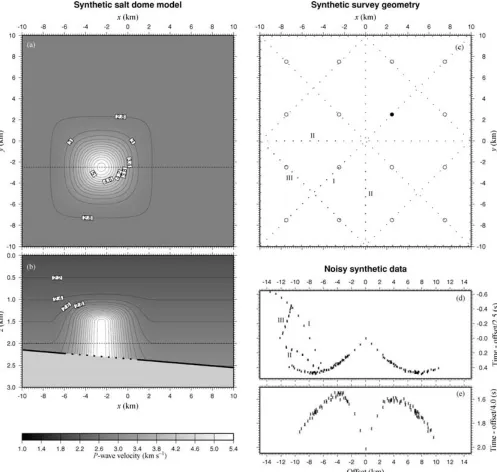
A practical inversion algorithm must be able to resolve structures which typically form targets in seismic surveys. In order to test the effectiveness of this algorithm in resolving a realistic structure, a synthetic test was devised using a model in which a salt dome intru-sion penetrated a sedimentary sequence containing a bright reflector. The salt dome model used here contained a velocity gradient repre-senting a sedimentary sequence approximately 2 km thick, bounded

Figure 4.Model, survey geometry and data for the synthetic salt dome experiment: (a) horizontal and (b) vertical cross-sections through the model used to generate synthetic data—the dotted section of the interface indicates the region in which no reflections were permitted to simulate disruption of the reflector by the dome; (c) geometry of the synthetic experiment, with 16 surface instruments (circles) and 290 shot points (dots). The data for a single instrument (solid circle) from all shots are plotted for (d) refracted and (e) reflected arrivals. The three refracted phases which pass through the salt dome are marked and correlated with their corresponding shot lines in (c).

at its base by a gently sloping reflector, interrupted by a salt dome intrusion of high seismic velocity. Two sections through the model are plotted in Figs 4(a) and (b). A synthetic data set was generated from this model using the forward-modelling method described in Section 2.2. A grid of instruments (‘sources’) was located at the model surface, and a set of intersecting lines was constructed along which shot points (‘receivers’) were placed at regular intervals. This geometry is illustrated in Fig. 4(c). No reflections were allowed from the interface within the area covered by the salt dome (in the region

−6<x<1,−6<y<1), simulating the disruption of the reflec-tor by the intrusion of the dome, and preventing the reflection data in this experiment from providing unrealistically good constraints

within the dome. Sets of normal-incidence, wide-angle reflection and wide-angle refraction traveltime data were generated from this model and experimental geometry between all source–receiver pairs for which solutions existed. Pseudo-random Gaussian noise with a constant standard deviation of 10 ms was added to all the traveltime data. The wide-angle data for a single instrument (containing all shots) are plotted in Figs 4(d) and (e), with the traveltimes reduced at constant velocity. In this plot, the sign for the offset was obtained from thex-coordinate of the shot point relative to the source, so the data characteristics at positive offset are influenced only by the constant gradient background velocity, while those at negative off-set also contain features caused by the presence of the salt dome. The refracted arrival curve contains three distinct phases produced by sampling the salt dome velocity structure along the three shot lines marked in Fig. 4(c). The effect of the dome on the reflected arrivals is less marked, and is manifest as a spread towards earlier traveltimes at negative offsets.

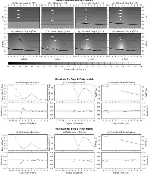
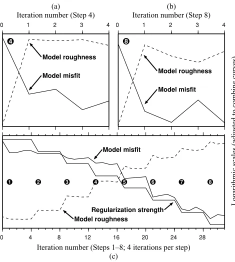
These data were inverted, employing the same velocity grid used to define the model (10×10×10 nodes) and a 10×10 node interface grid. A constant gradient, horizontal interface starting model was chosen in which the gradient and interface depth were both different from those in the real model. Noa prioriinformation was included in the form of, for example, weighting factors between the smoothing applied to velocity and interface functions, or between the lateral and vertical velocity smoothing. The inversion proceeded in 8 steps. Within each step, 4 iterations of forward-modelling and inversion were performed with the regularization strength held at a constant value. The regularization strength was then reduced for the following inversion step. A statistical analysis of the model evolution during inversion is shown in Fig. 6, and a series of vertical sections through the model as it evolved during inversion is shown in Fig. 5. The sections shown all follow the same slice as the vertical section in Fig. 4(b).

This model sequence bears close examination. During the first stage of the inversion (models a and b; the 1-D optimization), the average velocity, velocity gradient and interface depth all converge to values which minimize the data misfit. At this stage no lateral variation is allowed and the velocity function with depth is con-strained by regularization. An optimal 1-D model is obtained and the misfit considerably reduced. During the early stages of the 3-D optimization (models c and d), the features of the model emerge but are highly smoothed due to the strength of the regularization. At this stage the interface is well-positioned and its slope is correct, and the salt dome is beginning to emerge in the correct position. As the in-version proceeds (models e–h), the salt dome becomes increasingly well-defined. In the final model, for whichχ2 _{= 2, a satisfactory}

fit to the data, based on an examination of the traveltime residuals throughout data set, was judged to be close to being achieved. In fact, a stable solution withχ2_{=1 could not be found in this case—}

this was attributed to very high velocity gradients present within the salt dome, which could not be modelled satisfactorily using a single-layer model.

Residuals for a single section of wide-angle refraction and reflec-tion data and for normal-incidence data are plotted in Fig. 5, for an early model and the final model (steps 4 and 8). The early residuals are small at positive offsets, where the velocity and interface func-tions have correctly been determined, and larger at negative offsets, in the region of the salt dome, especially in the refracted arrivals. In the final model the residuals in this region are much improved, and the importance of the refraction data in determining the velocity structure of the dome may be seen by comparing plots (i) and (l) in Fig. 5.

Sections through the real and final models for this inversion are plotted together in Fig. 7 alongside a plot of uncertainties in the final velocity function, estimated using the method described in Section 2.4. A comparison between the discrepancy in the final model (the velocity in the real model minus the velocity in the final model) and the estimated uncertainty along a line through the salt dome is plotted in Fig. 8. The plot of uncertainties indicates, as expected, that the edges and deeper corners of the model are poorly constrained. There is also a region within the salt dome, in which the high velocity gradients cause seismic energy to be deflected away and in which no reflections were produced, with the result that the interior of the dome is poorly sampled. Fig. 8 indicates that the uncertainty in this area correctly indicates the extent to which velocities have been underestimated relative to the discrepancy in the surrounding area. At the model edges, where uncertainties are large, the actual discrepancy is small because the real model was smooth in these areas and an identical model has been constructed as a result of the smoothing regularization. Interestingly, the uncertainty analysis consistently overestimates the actual discrepancy in the final model, although it is a good indication of the relative uncertainties across the model. It is not clear whether such overestimation will always occur.

The salt dome inversion illustrates the most significant artefact introduced into models produced by the regularized least-squares inversion method. The later models in the sequence plotted in Fig. 5 all contain small fluctuations about an otherwise smooth model in the velocity contours away from the salt dome, and in the inter-face. Since the data constrain these areas to be completely smooth and the regularization applies additional smoothness constraints, the presence of these fluctuations requires some explanation. Their presence is due to an effect that resemblesGibbs’ phenomenon, or the behaviour of a damped simple harmonic system in response to a sudden change. Gibbs’ phenomenon is the ‘ringing’ effect that may be produced when high-frequency components are removed from some waveforms (e.g. a time-series square wave, which is constructed from an infinite series of sinusoidal components). The similarity with the phenomenon described here occurs because the smoothing process suppresses the highest frequency components of the velocity function. This ‘ringing’ is produced by the reg-ularized least-squares algorithm as it attempts to model a struc-ture in which the velocity gradients or gradients in interface depth are very high. The model produced is still the smoothest model that is able to fit the data to the selected level in a least-squares sense.

In the salt dome model (Fig. 5), the ringing emerges as the struc-ture of the salt dome begins to form (step 5) and increases as the dome boundaries are defined (step 6), then diminishes as the velocity structure within the dome is modelled. The ringing in the interface is introduced as a result of the velocity–depth trade-off which links the evolution of velocity and depth features. This ringing effect is illustrated for a simple 1-D velocity inversion in Fig. 9.

Figure 5.Evolution of the salt dome inversion showing (a) the starting model, (b) the results from the 1-D optimization and (c)–(h) results from the 3-D optimization at successively weaker regularization; also residuals from the salt dome inversion for (i,l) wide-angle refracted, ( j,m) wide-angle reflected and (k,n) normal-incidence arrivals, showing the traveltime data with error bars (points) overlain by synthetic data from step 4 and step 8 (lines), and the residuals plotted against the uncertainties in the data.

0 1 2 3 4 Iteration number (Step 4)

Model roughness

Model misfit 4

(a)

0 1 2 3 4

Iteration number (Step 8)

Model roughness

Model misfit 8

(b)

0 4 8 12 16 20 24 28

Iteration number (Steps 1–8; 4 iterations per step) Model roughness

Regularization strength Model misfit

1 2 3 4 5 6 7 8

(c)

Lo

garithmic scales (adjusted to combine cur

v

es)

Figure 6. Convergence statistics for synthetic inversion: Plots (a) and (b) illustrate the change in model misfit and model roughness over the four iter-ations of steps 4 and 8 of the inversion, showing a dramatic change in misfit and roughness during the first iteration followed by smaller adjustments char-acterized by a slight re-smoothing of the model and small oscillating changes in both measures caused by the trade-off between roughness and misfit dur-ing inversion. Plot (c) shows how the same quantities change throughout the eight inversion steps as the regularization strength steadily decreases.

4 A P P L I C A T I O N T O R E A L D A T A

The inversion method was applied to a real 3-D seismic data set acquired over the accretionary prism on the Cascadia Margin at approximately 49◦N. This is a region in which a strong and con-tinuous bottom-simulating reflector (BSR), the reflector normally associated with the presence of gas hydrate, has been observed in seismic reflection profiles (e.g. Hyndmanet al.1994).

The 3-D seismic data set was acquired in June 1993 on the CSS John P. Tully as a collaborative experiment between the University of Victoria, British Columbia and the University of Cambridge. Its primary objective was to image and to obtain constraints on the seismic velocity structure above and immediately below the BSR. The survey was centred around Ocean Drilling Program (ODP) Site 889B (Westbrooket al.1994). The data set used in this analysis was the result of two consecutive deployments of five ocean-bottom hydrophones (OBHs) on which wide-angle data were recorded on a number of profiles for offsets up to 13 km with simultaneous acquisition of single-channel reflection data from a hydrophone at the surface. The second deployment provided constraints at a higher resolution than the first (from a closer line and OBH spacing) with a shorter maximum offset. A single 120 cu. in. airgun source was used, for which the dominant source frequencies were 60–90 Hz. The most serious side-effect of this was the introduction of a strong bubble pulse throughout the entire data set. The hydrophone used to collect the single-channel data recorded at a sampling interval of 2 ms and the OBHs recorded at a sampling interval of 4 ms.

A subset of these data, recorded along a single acquisition line, was modelled by Hobroet al.(1998) in two dimensions using the

Figure 7. Vertical sections (aty = −2.5) through (a) the real salt dome model, (b) the final model from the inversion and (c) and (d) uncertainties for the final model.

-0.5 0.0 0.5 1.0 1.5 2.0 2.5 3.0 3.5 4.0 4.5 5.0

Uncer

tainty (km s

−

1)

-10 -8 -6 -4 -2 0 2 4 6 8 10

x (km)

Figure 8. Estimated uncertainty (solid line) and actual discrepancy (dotted line) for the final model plotted in Fig. 7, evaluated aty= −2.5 andz=

−1.5.

method of McCaughey & Singh (1997). In this study, a 2-D ve-locity model of a highly-deformed region of the survey area was successfully obtained from a combination of reflection and refrac-tion seismic data.

0.0 0.1 0.2 0.3 0.4 0.5 0.6 0.7 0.8 0.9 1.0

Depth (km)

1.0 1.1

Velocity (km s−1₎

(a)

1.0 1.1

Velocity (km s−1₎

(b)

1.0 1.1

Velocity (km s−1₎

(c)

1.0 1.1

Velocity (km s−1₎

(d)

1.0 1.1

Velocity (km s−1₎

(e)

1.0 1.1

Velocity (km s−1₎

(f)

1.0 1.1

Velocity (km s−1₎

(g)

0.0 0.1 0.2 0.3 0.4 0.5 0.6 0.7 0.8 0.9 1.0

Depth (km)

1.0 1.1

Velocity (km s−1₎

(h)

Figure 9.An illustration of the ringing effect produced by regularized least-squares when modelling well-constrained steep velocity gradients. A seismic source is located at the surface and direct arrival traveltimes are obtained for a series of receivers spaced regularly at 10 m depth intervals vertically beneath the source for the model plotted in (a). These times are then inverted using the regularized least-squares method at decreasing regularization strength (b–h). The velocity above the discontinuity at 0.5 km is well constrained, but below the discontinuity, interdependence in the model results in ringing. The asymmetry in this models obtained is due to the asymmetry in the geometry of the experiment.

Figure 10. Salt dome inversion results from two different starting models (a) and (d). During the 1-D optimization, the models converge to two indistinguishable solutions (b) and (e). The final results (c) and (f) are almost identical.

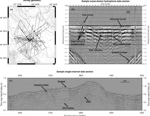
was centred on Site 889B. The shot spacing, which nominally re-mained constant throughout the survey, was approximately 35 m. A total of 112 of the 120 potential wide-angle OBH sections were recorded successfully and 99 of these yielded data that provided use-ful reflected and/or refracted traveltime picks. Samples of the wide-angle and single-channel seismic sections are plotted in Figs 11(b) and (c).

Traveltimes were picked from the OBH data (from horizons in-terpreted as BSR reflections and energy refracted in the sediments above the BSR) and the single-channel reflection data (seabed and BSR reflections). The inversion method described here was used ini-tially to construct an accurate model of the seabed using seabed picks from all the single-channel data (along all the lines in Fig. 11a) and a water velocity model based on conductivity–temperature–depth profiles. A seabed model more accurate than models provided by bathymetry data was required because the region contained large and complex variations in seabed topography (up to 1 km in depth).

In contrast, the target of the modelling process—the region between the seabed and the BSR—was only 200 m thick.

The seabed was parametrized as an interface spanning 25 km

×29 km, mapped using 100×100 depth nodes. These 10 000 model parameters were constrained in an inversion for the seabed structure by 9952 seabed reflection picks, obtained from the single-channel data in both deployments. A minimum-structure model that pro-vided a satisfactory fit to all the data was obtained. This seabed model illustrates well the properties of the regularized inversion ap-proach; areas of the model that are sparsely sampled by the data are interpolated smoothly, whereas complex structures exist where they are required to explain the data.

A sub-surface sedimentary velocity layer was defined over a 10 km×11 km×600 m volume that covered the well-sampled re-gion of the model. This volume was parametrized using 30×30×12 velocity nodes. The layer was bounded at its base by an interface that represented the BSR, which spanned the same lateral region as

Figure 11. (a) A plot of acquisition lines followed during the two wide-angle surveys with the positions of the OBHs indicated by dots; (b) sample OBH section reduced by ‘flattening’ the direct arrival, which shows the main features visible throughout the wide-angle data; (c) sample single-channel seismic section showing the seabed and BSR reflections.

the layer, and was parametrized by 30×30 depth nodes. The node density was chosen to reflect the maximum expected degree of struc-tural variation in the BSR and the seismic velocity field above. The expected complexity was estimated by examining the reflection data and considering the sampling limitations (e.g. Fresnel zone widths). Had a good fit to the data not been achieved using this parameter density, the data would have been re-modelled using a higher depth and velocity node density.

This model was used in a simultaneous inversion for sub-surface velocity and the depth of the BSR, with the water layer and seabed model fixed. A total of 12 446 traveltime picks were used (3042 single-channel BSR reflection picks, 3866 picks from turning rays above the BSR in the OBH data and 5538 BSR reflection picks from the OBH data). Since the general data quality and the clar-ity and coherence of individual horizons varied significantly across the data set, appropriate uncertainties were assigned individually to each data phase in each seismic section. Most of the single-channel reflection picks were assigned an uncertainty of±2.5 ms, an esti-mate of the picking uncertainty due to the bandwidth of the data recorded. In regions where the BSR was not strong, and in which the horizon, although identifiable, could not be picked without

intro-ducing a small amount of noise into the picked data, this uncertainty was increased to±4 ms. The normal-incidence constraints on the BSR constitute a dense coverage throughout the focal region of the survey (fromx≈11 km to 17 km and fromy≈17 km to 20 km), and a more sparse coverage elsewhere. Uncertainties for the BSR reflection phase in the OBH data ranged from±4 ms (the minimum uncertainty constrained by the bandwidth of the data) to±12 ms (a large uncertainty assigned where the precise location of the re-flection was not unambiguously identifiable). For the later refracted arrival in the OBH data, uncertainties ranged from±5 ms to±8 ms, and for the first arrival (which was in general less well-defined than the two later phases), from±12 ms to±20 ms. This data set provided a demanding test for a tomographic inversion method since the high velocity gradients and the presence of a strong shallow reflector generated a complex set of refracted and reflected horizons.

Figure 12. (a) a section through the final model showing variations in the velocity structure above the BSR (the dashed line marks the region in which velocities are well-constrained) with (b) velocity and (c) depth uncertainties; (d), (e), (f) and (g) traveltime residuals from sections of wide-angle and single-channel data, illustrating the quality of fit. Real and synthetic data are superimposed, and above each plot the residuals (black and grey dots) are compared with the uncertainties in each phase (refractions in grey and reflections in black).

traveltimes by adding a direct-arrival traveltime obtained by ray-tracing through the water column between the appropriate shot– instrument pair.

The inversion method was applied to these data, beginning with a 1-D inversion to determine the average BSR depth, sedimentary

P-velocity and velocity gradient, then allowing the regularization strength to decrease step by step as illustrated for the synthetic in-version in Fig. 6. The large variations in topography across the model caused significant lateral velocity gradients to emerge as the 1-D re-sult converged to a smooth 3-D intermediate model. A stable model convergence was achieved and a final model was chosen (after six steps) at the point where systematic components had been eliminated from the vast majority of data residuals (Figs 12d, e, f and g), leaving

only random noise. This indicated that the point had been reached where almost all structure in the data had been modelled without modelling any noise. The data residuals for the final model produced an overall fit ofχ2_{=0.76. A vertical cross-section through the most}

complex region of the final model is plotted in Fig. 12(a), with the corresponding plot of uncertainties in Figs 12(b) and (c) derived us-ing the method of Section 2.4. This model cross-section illustrates how the inversion method has resolved detailed structure in the well-constrained central region of the model, whereas the smoothing reg-ularization has stabilized the poorly-constrained model edges. The region of well-constrained seismic velocities marked in Fig. 12(a) is obtained from an isoline in the uncertainty function of Fig. 11(e) (at an uncertainty of±0.6 km s−1_).

A detailed analysis of this data set is presented by Hobro (1999). Detailed descriptions of the data set, its analysis, and interpretation of the final model are not presented here—the analysis of this data set is included in this paper in order to illustrate the ability of the inversion method described to model a detailed 3-D structure from real seismic data. The inversion method and data set are well-suited since, in this highly-deformed region with steep velocity gradients, the combination of reflection and refraction data provide consider-ably better constraints on the seismic velocity structure than either individual data type. In this example, a single iteration typically took around 4 minutes to complete the forward modelling phase, and a similar time to complete the inversion phase on a single Intel Pentium II 300 MHz CPU.

Further applications to real data sets have been presented by Funcket al.(2000) and Tonget al.(2002).

5 C O N C L U S I O N

A tomographic inversion method has been presented that obtains 3-D velocity–depth models from a range of reflection and refrac-tion seismic traveltime data types. The method makes simulta-neous use of reflection and refraction data in a constrained in-version that requires minimal user interaction and selects smooth minimum-structure models. The use of smooth basis functions in the model parametrization reduces the non-linearity in the forward-modelling and inversion schemes and consequently increases the robustness and efficiency of the method. Ray perturbation theory provides a semi-analytical method for forward-modelling through these smooth media. An inversion approach is adopted that allows the bulk properties of the model (average velocities, velocity gradi-ents and average interface depths) to be modelled initially with more detailed structure emerging as the inversion process continues. This provides an effective and objective approach to solving the highly non-linear tomographic problem whilst maintaining a high degree of independence from the starting model.

A series of tests on synthetic data were presented, from which it was concluded that:

(i) the method recovered a realistic target structure well from a set of noisy traveltime data,

(ii) the uncertainty analysis provided a useful assessment of the quality of constraint across the model, and

(iii) the final model recovered did not depend on the starting model used.

The method was applied to a real 3-D seismic data set containing co-incident seismic reflection and wide-angle data, the target of which was a region of the methane hydrate stability zone in the Cascadia Margin. A minimum-structure velocity–depth model of the region was obtained that provided a good fit to the traveltime data from all the phases picked. The results confirmed the ability of this method to model a complex seismic structure successfully at an efficient level of parametrization.

A C K N O W L E D G M E N T S

We would like to thank George Spence and all involved in the Tully 1993 cruise for acquiring the data set presented here, which was funded by NSERC in Canada and NERC in the UK. J. Hobro was supported by a NERC research studentship and T. Minshull by a Royal Society University Research Fellowship. We thank Jay Pulliam and Colin Zelt for thorough reviews.

R E F E R E N C E S

Aki, K. & Lee, W.H.K., 1976. Determination of three-dimensional velocity anomalies under a seismic array using firstParrival times from local earthquakes,J. geophys. Res.,81,4381–4399.

Buchanan, J.L. & Turner, P.R., 1992.Numerical Methods and Analysis, McGraw-Hill, Inc.

Catchings, R.D. & Mooney, W.D., 1988. Crustal structure of the Columbia Plateau: evidence for continental rifting, J. geophys. Res., 93, 459– 474.

ˇ

Cerven´y, V., 1987. Ray tracing algorithms in three-dimensional laterally varying layered structures, inSeismic Tomography, with Applications in Global Seismology and Exploration Geophysics,ed. Nolet, G., Reidel, Dordrecht.

ˇ

Cerven´y, V., Molotkov, I.A. & Psencik, I., 1977.Ray Method in Seismology, University of Karlova Press, Prague.

Chapman, C.H., 1985. Ray theory and its extensions: WKBJ and Maslov seismograms,J. Geophys.,58,27–43.

Constable, S.C., Parker, R.L. & Constable, C.G., 1987. Occam’s inversion: A practical algorithm for generating smooth models from electromagnetic sounding data,Geophysics,52,289–300.

Eberhart-Phillips, D., 1986. Three-dimensional velocity structure in northern California Coast Ranges from inversion of local earthquake arrival times, Bull. seism. Soc. Am.,76,1025–1052.

Firbas, P., 1987. Tomography from seismic profiles, inSeismic Tomography, with Applications in Global Seismology and Exploration Geophysics,ed. Nolet, G., Reidel, Dordrecht.

Funck, T., Louden, K.E., Wardle, R.J., Hall, J., Hobro, J.W.D., Salisbury, M.H. & Muzzatti, A., 2000. Three-dimensional structure of the Torngat Orogen (NE Canada) from active seismic tomography,J. geophys. Res., 105,23 403–23 420.

Ghose, S., Hamburger, M.W. & Virieux, J., 1998. Three-dimensional velocity structure and earthquake locations beneath the northern Tien Shan of Kyrgyzstan, central Asia,J. geophys. Res.,103,2725–2748.

Henry, W.J., Mechie, J., Maguire, P.K.H., Khan, M.A., Prodehl, C., Keller, G.R. & Patel, J., 1990. A seismic investigation of the Kenya Rift Valley, Geophys. J. Int.,100,107–130.

Hestenes, M. & Stiefel, E., 1952. Methods of conjugate gradients for solving linear systems,Nat. B. Stand. J. Res.,49,409–436.

Hobro, J.W., Minshull, T.A. & Singh, S.C., 1998. Tomographic seismic studies of the methane hydrate stability zone in the Cascadia Margin, in Gas Hydrates: Relevance to World Margin Stability and Climate Change, Vol. 137, pp. 133–140, Geological Society, London.

Hobro, J.W.D., 1999. Three-dimensional tomographic inversion of combined reflection and refraction seismic traveltime data,PhD thesis,Department of Earth Sciences, University of Cambridge, Cambridge.

Holbrook, W.S., Reiter, E.C., Purdy, G.M., Sawyer, D., Stoffa, P.L., Austin, J.A, Oh, J. & Makris, J., 1994. Deep structure of the U.S. Atlantic con-tinental margin, offshore South Carolina, from coincident ocean bottom and multichannel seismic data,J. geophys. Res.,99,9155–9178. Hole, J.A., 1992. Nonlinear high-resolution three-dimensional seismic travel

time tomography,J. geophys. Res.,97,6553–6562.

Huang, H., Spencer, C. & Green, A., 1986. A method for the inversion of re-fraction and reflection traveltimes for laterally varying velocity structures, Bull. seism. Soc. Am.,76,837–846.

Hyndman, R.D., Spence, G.D., Yuan, T. & Davis, E.E., 1994. Regional geo-physics and structural framework of the Vancouver Island margin ac-cretionary prism, inProc. ODP, Init. Rept.,146, Part 1. 399–419, eds Westbrook, G.K., Carson, B. & Musgrave, R.J.,et al.

Korenaga, J., Holbrook, W.S., Kent, G.M., Keleman, P.B., Detrick, R.S., Larsen, H.C., Hopper, J.R. & Dahl-Jensen, T., 2000. Deep structure of the U.S. Atlantic continental margin, offshore South Carolina, from coinci-dent ocean bottom and multichannel seismic data,J. geophys. Res.,105, 21 591–21 614.

McCaughey, M. & Singh, S.C., 1997. Simultaneous velocity and interface tomography of normal-incidence and wide-aperture seismic traveltime data,Geophys. J. Int.,131,87–99.

Moser, T.J., 1991. Shortest path calculations of seismic rays,Geophysics, 56,59–67.

Ni, J.F., Ibenbrahim, A. & Roecker, S.W., 1991. Three-dimensional velocity structure and hypocenters of earthquakes beneath the Hazara arc, Pakistan: Geometry of underthrusting Indiana plate,J. geophys. Res.,96,19 865– 19 877.

Nolet, G., 1987. Seismic wave propagation and seismic tomography, in Seis-mic Tomography, with Applications in Global Seismology and Exploration Geophysics,ed. Nolet, G., Reidel, Dordrecht.

Robertsson, J.O.A., Blanch, J.O. & Symes, W.W., 1994. Viscoelastic finite-difference modeling,Geophysics,59,1444–1456.

Shaw, P.R. & Orcutt, J.A., 1985. Waveform inversion of seismic refraction data and applications to young pacific crust,Geophys. J. R. astr. Soc.,82, 375–414.

Spence, G.D., Clowes, R.M. & Ellis, R.M., 1985. Seismic structure across the active subduction zone of western Canada,J. geophys. Res.,90,6754– 6772.

Tarantola, A., 1987.Inverse Problem Theory: methods for data fitting and model parameter estimation,Elsevier, Amsterdam.

Tikhonov, A.N. & Arsenin, V.Y., 1977.Solutions of Ill-posed Problems,

Wiley, New York.

Tong, C.H.et al., 2002. Asymmetric melt sills and upper crustal construction beneath overlapping ridge segments,Geology,30,83–86.

Toomey, D.R., Solomon, S.C. & Purdy, G.M., 1994. Tomographic imag-ing of the shallow crustal structure of the east pacific rise at 9◦30n,J. geophys. Res.,99,24 135–24 157.

Virieux, J. & Farra, V., 1991. Ray tracing in 3-D complex isotropic media: An analysis of the problem,Geophysics,56,2057–2069.

Wang, B. & Braile, L.W., 1996. Simultaneous inversion of reflection and refraction seismic data and application to field data from the northern Rio Grande rift,Geophys. J. Int.,125,443–458.

Westbrook, G.K., Carson, B., Musgrave, R.J.et al., eds., 1994.Proc. ODP, Init. Rept,146,(Part 1).

Williamson, P.R., 1990. Tomographic inversion in reflection seismology, Geophys. J. Int.,100,255–274.

Zelt, C.A. & Barton, P.J., 1998. Three-dimensional seismic refraction to-mography: A comparison of two methods applied to data from the Faroe Basin,J. geophys. Res.,103,7187–7210.

Zelt, C.A. & Smith, R.B., 1992. Seismic traveltime inversion for 2-D crustal velocity structure,Geophys. J. Int.,108,16–34.

Zhang, J., ten Brink, U.S. & Toks¨oz, M.N., 1998. Nonlinear refraction and reflection traveltime tomography, J. geophys. Res.,103, 29 743– 29 757.