Towards robust evolutionary inference with integral projection models

models

Maria Jo˜ao Janeiro

_{, David W. Coltman}

_{, Marco Festa-Bianchet}

_{, Fanie Pelletier}

_{, and}

Michael B. Morrissey

1

_{School of Biology, University of St Andrews, St Andrews, Fife, United Kingdom}

_{CESAM, Department of Biology, University of Aveiro, Aveiro, Portugal}

3

_{D´epartement de biologie, Facult´e des Sciences, Universit´e de Sherbrooke, Sherbrooke,}

Qu´ebec, Canada

4

_{Department of Biological Sciences, University of Alberta, Edmonton, Alberta, Canada}

_{corresponding author, email: [email protected]}

Abstract 1

Integral projection models (IPMs) are extremely flexible tools for ecological and evolutionary infer-2

ence. IPMs track the distribution of phenotype in populations through time, using functions describing 3

phenotype-dependent development, inheritance, survival and fecundity. For evolutionary inference, two 4

important features of any model are the ability to (i) characterize relationships among traits (including 5

values of the same traits across ages) within individuals, and (ii) characterize similarity between indi-6

viduals and their descendants. In IPM analyses, the former depends on regressions of observed trait 7

values at each age on values at the previous age (development functions), and the latter on regressions 8

of o↵spring values at birth on parent values as adults (inheritance functions). We show analytically that 9

development functions, characterized this way, will typically underestimate covariances of trait values 10

across ages, due to compounding of regression to the mean across projection steps. Similarly, we show 11

that inheritance, characterized this way, is inconsistent with a modern understanding of inheritance, and 12

underestimates the degree to which relatives are phenotypically similar. Additionally, we show that the 13

use of a constant biometric inheritance function, particularly with a constant intercept, is incompati-14

ble with evolution. Consequently, current implementations of IPMs will predict little or no phenotypic 15

evolution, purely as artifacts of their construction. We present alternative approaches to constructing 16

development and inheritance functions, based on a quantitative genetic approach, and show analytically 17

and through an empirical example on a population of bighorn sheep how they can potentially recover 18

patterns that are critical to evolutionary inference. 19

20

Keywords: integral projection models, regression to the mean, inheritance, development, body size, 21

Introduction

23

Evolutionary and ecological dynamics converge at the scale of generation-to-generation change in popula-24

tions (Pelletier et al., 2009; Coulson et al., 2010). When traits cause fitness variation, the distributions of 25

those traits, weighted by fitness, necessarily changes within generations (Godfrey-Smith, 2007). If di↵erences 26

among individuals have a genetic basis, then genetic changes will be concomitant with phenotypic changes. 27

Such genetic changes are the basis for the transmission of within-generation change due to selection, to ge-28

netic change between populations, i.e. evolution (Lewontin, 1970; Endler, 1986). The fundamental nature of 29

this relationship between phenotypic change due to selection, and associated genetic and thus evolutionary 30

change, has motivated the development of various expressions relating selection to genetic variation and 31

evolution in quantitative terms (Lush, 1937; Robertson, 1966, 1968; Lande, 1979; Lande & Arnold, 1983; 32

Morrissey, 2014, 2015). Important recent advances in population demography, particularly the introduction 33

(Easterling et al., 2000) and popularization (e.g. Childs et al., 2003; Ellner & Rees, 2006; Coulson et al., 2010; 34

Ozgul et al., 2010; Coulson, 2012; Merow et al., 2014) of integral projection models (IPMs), can potentially 35

allow the construction of very flexible models of changes in phenotype, and of its associated demographic 36

implications (Coulson et al., 2010). 37

38

IPMs are structured population models used to study the dynamic of populations when individuals’ vital 39

rates (e.g. survival, growth, reproduction) depend on one or more continuous state variables (e.g. mass). 40

In principle, these model structures track the distribution of individual values of the state variables through 41

time. To achieve this, IPMs make population projections from regression models that define the underlying 42

vital rates as a function of the state variables. Four core sets of functions for vital rates have been defined, 43

termed fundamental functions or fundamental processes (Coulson et al., 2010): (i) survival, (ii) fertility, (iii) 44

ontogenetic development of focal trait conditional on surviving (development functions), and (iv) distribu-45

tion of o↵spring trait as a function of parental trait (inheritance functions). In principle, the inheritance 46

functions allow IPMs to be used to make evolutionary inference, i.e. inference of evolutionary trajectories 47

and parameters relevant to evolutionary processes, such as selection and genetic variation, particularly in-48

cluding the estimation of biometric heritabilities (Coulson et al., 2010; Schindler et al., 2013; Traill et al., 49

2014; Bassar et al., 2016). As discussed by Coulson et al. (2010), these four processes underlie the high flex-50

ibility of IPMs and their ability to link di↵erent aspects of population ecology, evolutionary biology and life 51

history. The fundamental processes are combined to compute a function called the kernel, which represents 52

all possible transitions between state values through time (e.g. the probability density of transitions from 53

t 1 is integrated over all possible sizes to obtain the number of individuals of sizex2 at timet. In general, 55

the numerical implementation of IPMs involves the construction of an iteration matrix to solve the integral. 56

Empirical examples include the study of monocarpic plant species (Childs et al., 2003; Rees et al., 2006; 57

Ellner & Rees, 2006), Soay (Ovis aries, Ozgul et al. 2009; Childs et al. 2011) and bighorn (Ovis canadensis, 58

Traill et al. 2014) sheep, yellow-bellied marmots (Marmota flaviventris, Ozgul et al. 2010), and Trinidadian 59

guppies (Poecilia reticulata, Bassar et al. 2016). 60

61

A key aspect of the distribution of phenotypes is how traits covary at the level of individuals. Genetic and 62

phenotypic covariances among traits are key determinants of evolution (Lande, 1979). In the context of 63

IPMs, which often consider single traits (e.g. mass), age-specific values of a given trait can be thought of as 64

separate, age-specific traits, the covariances among which are key determinants of evolutionary processes. In 65

fact, in these models, when selection acts only on juveniles, evolution can only occur if there is covariance 66

between trait values at juvenile ages and some aspect (genetic or phenotypic) of the state of individuals 67

at the stage when they reproduce. Such mechanics di↵er from the classic quantitative genetic approach, 68

where a change in phenotype is transmitted to future generations if there is a change in breeding values. 69

In most IPMs as parameterized to date (e.g. Childs et al., 2003; Ellner & Rees, 2006; Coulson et al., 2010; 70

Ozgul et al., 2010), recovering covariance across ages depends on correctly estimating regressions of observed 71

trait values at each age on trait values at the previous age. In practice, as it is well known, such regres-72

sions will typically be underestimated due to regression to the mean (Campbell & Kenny, 1999; Barnett 73

et al., 2005; Kelly & Price, 2005). This statistical phenomenon - unusually extreme measurements being 74

followed by measurements that are closer to the mean - is a manifestation of measurement error. Regression 75

to the mean therefore occurs if phenotypic measurements of predictor variables imperfectly reflect relevant 76

biological quantities. This problem has begun to be investigated in the context of IPMs (Chevin, 2015), 77

and it is likely to be very general. The development functions used so far in IPMs estimate size at any 78

age as an accumulation of growth from birth until that age, which implies that size at age a is estimated 79

through a series of regressions in which an increasing measurement error in the predictor is not accounted 80

for. We note that IPMs do not imply the occurrence of regression to the mean. The issues that we dis-81

cuss in this article are related to the statistical models that are typically - but not necessarily - used in IPMs. 82

83

In age-size-structured IPMs, size-dependent transition functions of the fundamental demographic processes 84

are used to project size distribution from one age to the next, and across generations. The inheritance 85

function has been defined as an association between the phenotype of the o↵spring as newborns or juveniles 86

Traill et al., 2014; Bassar et al., 2016). Essentially, it is a cross-age parent-o↵spring regression, which is a 88

peculiar measure of resemblance due to inheritance. Outside of the IPM framework, the concept of biometric 89

heritability - the slope of the o↵spring trait regressed on the midparent’s value (Jacquard, 1983) - is defined 90

by comparing parent and o↵spring at the same age (e.g. Galton, 1886). In fact, no theory exists for the 91

concept of cross-age heritability as used in IPMs. Body size, commonly the focal trait in IPMs, is typically 92

a dynamic trait (a trait that varies over the development) and therefore its value at a certain age is the 93

result of the accumulation of growth until that age, causing di↵erences among individuals to accumulate 94

over the ontogeny due to environmental and genetic variation in size trajectories (Chevin, 2015). As genes, 95

not phenotypes resulting from development, are inherited, parental phenotype as an adult is an imperfect 96

predictor of the parental genetic contribution to the o↵spring phenotype. As a consequence of phenotype 97

being used as a predictor, regression to the mean occurs and results in the underestimation of resemblance 98

between parents and their o↵spring, and therefore of the genetic contribution to phenotypic change (Chevin, 99

2015). 100

101

Here we construct simple but realistic theoretical models of development and inheritance of a quantitative 102

phenotypic trait. For both development and inheritance, we also construct corresponding models to the 103

functions normally implemented in IPMs. By comparing these two sets of models, we investigate how the 104

development and inheritance functions adopted to date in IPMs use data on size-at-age of relatives, and 105

how well they recover across-age and across-generation population structure in continuous traits. Aspects 106

of the distribution of traits through time, other than over single iteration steps, in size-dependent devel-107

opment and inheritance functions, are normally not used to parameterize IPMs. Also, IPMs are typically 108

iterated so that once the population structure at timet+ 1 is generated, the state of the population at time 109

t is discarded. Consequently, while IPMs’ most important feature is tracking the distribution of phenotype 110

through time, they do not output aspects of population structure (e.g. correlations in size within individuals 111

across ages) that allow their performance to be checked. This is a critical point because whenever aspects 112

of the distribution of traits across time are of interest for any inference, particularly evolutionary inference, 113

correlations of individual trait values across ages, and of trait values of relatives across generations, must 114

be adequately reflected. Path analysis (McArdle & McDonald, 1984) can be very useful in studying such 115

correlations. In fact, the structure of both the development functions with their autoregressive structure -116

and of the biometric inheritance - with associations both among di↵erent generations and among di↵erent 117

ages - can be conveniently illustrated by a path diagram representing the causal relationships amongst a set 118

of variables. Also, the path (or tracing) rules are easily applied to obtain the correlations among variables 119

to generate analytical expressions that isolate growth and inheritance, providing insight into the degree to 121

which models of these processes typically used to date recover the structure of populations. 122

123

We demonstrate that current parameterizations of IPMs generally recover only a small fraction of the true 124

underlying similarity within individuals across ages (sectionDevelopment), and a small fraction of the true 125

underlying similarity between relatives (sectionInheritance). These shortcomings have severe consequences 126

for evolutionary inference with IPMs. We then provide an empirical example of a quantitative genetic anal-127

ysis of developmental trajectories in a pedigreed wild population of bighorn sheep using a random regression 128

animal model of body mass. We compare the random regression analysis, which not only should be robust to 129

regression to the mean, but also uses a model of inheritance based on established principles of how biometric 130

relationships among kin arise from genetic variation (Fisher, 1918; Wright, 1921), to the inheritance function 131

based on the cross-age parent-o↵spring regression and standard regression methods for growth functions 132

normally implemented into IPMs. We show a large di↵erence between the two parameterizations in the 133

ability to capture similarity within individuals across ages, which results in standard regression methods 134

normally used in IPMs not capturing the across-age structure in growth. Similar conclusions are reached 135

across generations, where IPMs miss most similarity among relatives, corresponding to a failure of the typical 136

IPM inheritance function to predict evolution. We conclude by discussing the results from the theoretical 137

and empirical sections and potential solutions that may prove useful in fully realizing the potential of IPMs. 138

139

Development

140

Regression to the mean is particularly relevant to IPMs due to how size-dependent growth coefficients are 141

typically - although not necessarily - estimated. Transition rates between size classes for surviving individuals 142

are modelled by regressing observed size at agea+ 1 on observed size at agea, observed size being therefore 143

a predictor. Either linear models (e.g. Childs et al., 2003; Coulson et al., 2010), or extensions of such models, 144

including generalized linear or additive (mixed) models and nonlinear models (e.g. Ozgul et al., 2010; Rees 145

et al., 2014; Traill et al., 2014) have been used for this purpose. All these methods assume that predictors 146

are measured without error. When this assumption is violated, downwardly biased estimates are obtained 147

(for a review on problems and proposed models to deal with measurement error see Thompson & Carter, 148

2007). Measurements of most traits, including size, will virtually always be made with non-trivial error, for 149

two reasons. First, limitations in the measurement process caused by di↵erent measuring conditions (e.g. 150

measurement, tend to occur. Second, size, like most other variables of ecological interest, is an abstract 152

concept and therefore is not directly measurable. As such, proxy variables that do not perfectly represent 153

size are measured instead, such as mass or some skeletal measure. The complexity ofsize is such that the 154

covariation between any proxy at timetandt+ 1 is also determined by the other components of size, which 155

are highly correlated with each other. Importantly, the mechanics underlying IPMs neither imply measure-156

ment error nor regression to the mean. Rather, the application of standard regression methods that do not 157

account for measurement error within an autoregressive structure on size (subsequent sizes being used as 158

predictors) promotes the occurence of regression to the mean due to measurement error. 159

160

Since the measurement error that causes regression to the mean is random rather than systematic, this 161

problem can be modelled by thinking of true size, the trait we want to measure, as a latent variable,z, that 162

cannot be measured (e.g. McArdle, 2009; Little, 2013, p. 43). In such a scenario, instead of the true values 163

z, a proxy, the trait we actually measure,x, is recorded, which di↵ers fromz by a measurement error, 2

✏,

164

and is related to it by a repeatability, r2_{. x can, therefore, be written as x = z+} 2

✏. In figure 1A, we

165

illustrate such model of the ontogenetic development of size, which we namedlatent true size model, using 166

a path diagram. In this diagram, true size at age 1, z1, determines true size at age 2, z2. z2 is then a 167

predictor of true size at age 3, z3, and so on until size at age n, zn, is predicted. In contrast, the kinds 168

of regression analyses implemented to date in IPMs (e.g. Childs et al., 2003; Coulson et al., 2010; Ozgul 169

et al., 2010; Rees et al., 2014; Traill et al., 2014) assume that true sizez is being measured when in fact the 170

measured variable isx. This model, which we termedobserved size model, is illustrated in figure 1B. The 171

autoregressive structure in this model is very similar to that in figure 1A, but is built on observed sizes rather 172

than true ones. We use the theoretical models in figure 1 to illustrate the consequences of this conceptual 173

mismatch and to inspect how regression to the mean a↵ects inference about development. We show that the 174

correlations, and therefore the regression coefficients, estimated using IPMs do not correspond to the true 175

latent ones. We then derive a generic analytical expression for how much correlation an IPM can recover 176

given a certain repeatability and number of projection steps (number of IPM iterations). 177

178

If we consider linear size-dependent growth functions, we can express the true biometric relationships (i.e. 179

true theoretical expressions) among traitsz(e.g. size at di↵erent ages), as well as the relationships captured 180

by standard regression methods typically used in IPMs to describe development, using the principles of 181

path analysis (McArdle & McDonald, 1984). Developed by Wright (1921, 1934) for estimating causal path 182

coefficients, path analysis mathematically decomposes correlations (or covariances) among the variables in 183

dardized (mean centered and variance of 1). In such circumstances, the expected correlation between two 185

variables is the product of the standardized path coefficients that link them. Some notational details are 186

worth summarizing: denotes several aspects of true covariation (covariance in growth among ages), whereas 187

2 _{represents true variances. Variances estimated by IPMs are denoted bys}2_{. Since the models in figure 1}

188

are antedependence models (or autoregressive, as the response variable depends on itself at a previous time), 189

2

g in figure 1A ands2g in in figure 1B correspond to variances in growth associated with the regressions of 190

true size on true size at a previous time and observed size on observed size at a previous time, respectively. 191

Finally, the path coefficientsbcorrespond to regressions of size on size andr2_{to the square of the regression}

192

coefficient of observed size at agea, xa, on true size at the same age, za. Following the principles of path 193

analysis, we used a variance-covariance matrix with the variances in growth, 2

ga, and errors associated

194

with observed sizes, 2

✏a, for each agea, and a matrix with path coefficients (bz a and ra) matching figure

195

1A to obtain a variance-covariance matrix for sizes at di↵erent ages (Appendix A1). From this matrix, we 196

then extracted the covariances among ages for both true and observed sizes (Table B.1 in appendix B). As 197

an example, according to the path rules, the correlation and covariance in true size between ages 1 and 198

3 are given by bz1·bz2 and 2g1·bz1·bz2, respectively. Analogous quantities were obtained similarly for

199

IPMs (Table B.2 in appendix B). Since regressions of observed size on observed size,bxa, are estimated from

200

the data (rather than implied), these quantities are necessarily recovered correctly, and therefore the bxa

201

estimated in IPMs (figure 1B) are equivalent to the analogous quantities in figure 1A. In contrast, variances 202

in growth estimated with observed sizes,s2

ga, do not correspond to variances in growth estimated with true

203

latent sizes, 2

g a, nor to the measurement error associated with observed sizes, ✏2a. Consequently, since these 204

quantities are crucial to estimate covariances in size among ages, the across-age distribution of phenotype 205

that occurs in a typically-constructed IPM does not generally recover the across-age distribution of either a 206

measured aspect of phenotype (e.g. correlations in thexvariable across ages) or of an underlying quantity 207

(e.g. correlations in the z variable across ages). An across-age distribution of phenotype, which includes 208

correlations among ages, is not typically tracked by an IPM (e.g. Childs et al., 2003; Ellner & Rees, 2006; 209

Coulson et al., 2010; Ozgul et al., 2010). Yet, an IPM’s utility for any ecological and evolutionary inference 210

depends on its ability to track this distribution through time. In a typical implementation, the distribution 211

of phenotype at agea 1 is discarded once the distribution at ageais generated, so such correlations cannot 212

easily be outputted and checked against data. As such, we use path analysis to mimic basic IPM mechanics 213

and to extract the across-age dynamics that are not otherwise easily tracked. In contrast, an IPM can easily 214

be interrogated for the distribution of phenotype at any given time. These distributions generally closely 215

match data (Ozgul et al., 2010; Childs et al., 2011, also see fig3(a) in Chevin, 2015 for a simulation example). 216

For tractability, we demonstrate that IPMs do not in general recover the across-age structure of phenotype 218

using a simplified case of the path diagram in figure 1A as the true model. Specifically, we focus on a 219

static trait, as it renders the basic principles more clearly without loss of generality. We assume that all 220

size-dependent growth coefficients are one (bza= 1,8a), that the variance in true growth at age one - which

221

also corresponds to the variance in true size at age one - is one ( 2

g1= 1) and that the subsequent variances

222

are zero ( 2

ga = 0,8a > 1). Finally, all repeatabilities, ra, and measurement errors, 2

✏a, take the same

223

value, r and 1 r2_{, respectively. Applying the path rules and these assumptions results in the particular}

224

case of all true phenotypic variances and covariances being 1 and variances and covariances for phenotypic 225

observed size being 1 and r2_{, respectively (see appendix A.1.2 for details). Standard regression methods}

226

typically used in IPMs underestimate regressions for true growth in any instance where r <1, by a factor 227

of r2_{. Whenever true and observed sizes di↵er, which is true for virtually every attempt to measure size,}

228

instead of 1 (value set for allbza),bxatake the valuer

2_{for any consecutive pair of ages (both in figure 1A and}

229

1B). As mentioned before, covariances in size across ages are in general not reported when building an IPM. 230

However, the implied covariances can be calculated using path analysis (see appendix A.1.1 for the general 231

case and appendix A.1.2 for this simplified example). Since according to the path rules of standardized 232

variables correlations between two variables correspond to the product of the path coefficients linking them, 233

in this example correlations in size among two ages will be r2 _{to a power equivalent to the number of links}

234

between them. As such, sincer <1, these correlations will be underestimated. As for the covariances, these 235

are obtained by multiplying the correlations by the variance in growth at age 1, which corresponds to the 236

variance in growth at age one,sg1. Variances in size are well recovered in IPMs because these quantities are

237

directly estimated from the data. Therefore, in this example,sg1, which also corresponds to variance in size

238

at age one, corresponds to one, resulting in covariances in size implied by the growth functions normally 239

implemented in IPMs being given by 240

covIP M(xi, xj) = r2 t, (1)

where

t

242

The standardized conditions set in this simplified example illuminate how much correlation between sizes at 243

di↵erent ages the standard IPM formulation will miss. As true correlations (or covariances) in size across 244

ages were set to one, subtracting the correlation in equation (1) to that theoretical value corresponds to the 245

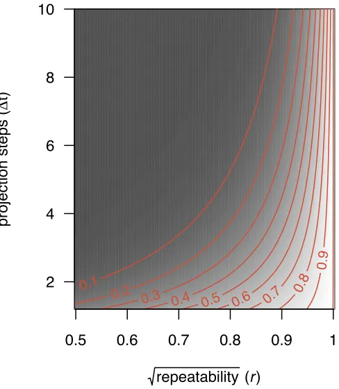
missed correlation = 1 r2 t . (2)

The theoretical result of equation (2) shown in figure 2 demonstrates that this quantity is far from negligible, 247

increasing rapidly with the number of projection steps and decreasing values of r. Many IPM analyses to 248

date have focused on long-lived organisms. In these systems, age di↵erences (projection steps) of 5 to 10 249

years may correspond to the gap between juvenile stages, which are often subject to the strongest viability 250

selection, and ages of greatest fecundity. Even for traits with high repeatabilities (e.g. r= 0.9), correlations 251

over such age di↵erences will be underestimated by more than 60% (Figure 2). Ultimately, size is estimated 252

as an accumulation of growth through an autoregressive process that discards the distribution of size at 253

time t 1 at each iteration (when the distribution att is obtained). This results in measurement error at 254

each iteration not being accounted for in the next, and therefore the e↵ect of regression to the mean rising 255

with the number of IPM projection steps. Serious consequences can be expected both for evolutionary and 256

ecology studies, whenever di↵erences in individual growth are of interest. Curiously, all else being equal, 257

IPMs with narrower projection intervals (e.g. monthly, rather than yearly) will su↵er more from regression 258

to the mean than models constructed with wider projection intervals. Finally, it is important to note that 259

asserting that the observed quantities, rather than underlying variables, are the target of interest in any 260

given IPM application does not solve the fundamental problem. In any scenario where the covariance of 261

observed values through time is caused (in part or in whole) by quantities other than the observed values 262

themselves (figure 1A) a model of sequential regressions of observed values on one another (figure 1B) will 263

not recover the resulting covariance structure. 264

265

Inheritance

266

The modern understanding of how genes contribute to similarity among relatives (Fisher, 1918, 1930; Wright, 267

1922, 1931) has a very di↵erent structure from the inheritance function typically included in IPMs (e.g. 268

Coulson et al., 2010; Traill et al., 2014; Bassar et al., 2016). Fisher and Wright showed how Mendelian 269

inheritance at many loci influencing a trait generates the observed biometric relationships among relatives, 270

including the relationships of a quantitative character between parents and o↵spring. Here, we use the basic 271

mechanics of inheritance of a polygenic trait, which have well-known relationships to selection and evolution 272

(Walsh & Lynch, forthcoming), and use it as simple background to see if IPM mechanics are generalizations 273

theory of the inheritance of quantitative traits, and has its roots in Fisher’s (1918) and Bulmer’s (1980) 275

infinitesimal model (see Falconer, 1981; Walsh & Lynch, forthcoming, Chapter 15). Each parent passes half 276

of its genes and therefore half of its breeding value on to the o↵spring. As such, the expected breeding value 277

of o↵springi,E[BVi], corresponds to half the sum of parental breeding values, as follows 278

E[BVi] = (BVmi+BVfi)

2 , (3)

whereBVmi andBVfi are the maternal and paternal breeding values, respectively. The true breeding value,

279

BVi, follows a normal distribution, 280

BVi⇠N(E[BVi],

2

a

2 ), (4)

with its expected value as mean and ₂2

a

the absence of inbreeding, conditional on mid-parent breeding values, resulting from segregation (Bulmer, 282

1980). The variance in the breeding values divided by the phenotypic variance is defined as heritability,h2_,

283

a measure of evolutionary potential. The degree of resemblance between relatives provides the means for 284

distinguishing the di↵erent sources of phenotypic variation and therefore for estimating heritabilities and 285

other quantitative genetic parameters (Falconer, 1981). The simplest way of doing so is by using correlations 286

of close kin, for example, of parents and their o↵spring, as h2 _{corresponds to the slope of the o↵spring}

287

trait regressed on the midparent’s (Lynch & Walsh, 1998, Chapter 7). In fact, Jacquard (1983) defines the 288

heritability estimated with a parent-o↵spring regression as a biometric heritability, as opposed to broad- and 289

narrow-sense heritabilities, for which the genetic and additive genetic variances are, respectively, explicitly 290

estimated. Any genetic architecture, i.e. broad- and narrow-sense heritability, determines the biometric 291

relationships among kin (Lynch & Walsh, 1998, Table 7.2). In IPMs, heritabilities have been estimated 292

using parent-o↵spring regressions. Specifically, inheritance has been defined as a regression of the phenotype 293

of the o↵spring as newborns or juveniles on that of the parents at the time the o↵spring was produced 294

(Coulson et al., 2010; Schindler et al., 2013; Traill et al., 2014; Bassar et al., 2016). In this section, we 295

investigate whether this cross-age biometric notion of inheritance is compatible with what is known about 296

trait transmission across generations. 297

298

Inheritance across generations

299

We start by addressing consequences of regression to the mean related to the biometric concept of inheritance 300

tions of the same age, according to Fisher’s and Wright’s understanding of trait transmission (Figure 3A), 302

and a comparable model reflecting the biometric concept of inheritance typically used in IPMs (Figure 3B). 303

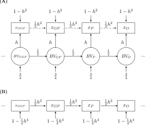
As for the development models, we used path diagrams and path analysis to compare the correlations implied 304

by both models. In figure 3A, breeding values, the underlying units that are inherited, are passed on across 305

generations: from great-grandparents to grandparents, from grandparents to parents, and from these to the 306

o↵spring. Since each parent passes on half its breeding value to the next generation, the regression coefficient 307

linking generations is 1

2. The variance associated with the breeding values is 3

4, which corresponds to 1 2 from

308

the other parent and 1₄ from segregation. h corresponds to correlation between the breeding values and 309

phenotypic values (Wright, 1921; Falconer, 1981) and, in a standardized path analysis, to the corresponding 310

regression coefficient as well. If observed size is standardized (variance of 1), then according to the path rules 311

its exogenous variance corresponds to 1 h2_{. Finally, if any regression was to be made between the observed}

312

sizes,x, the coefficient would be half the heritability. There is a close analogy with the path diagrams in figure 313

3A and figure 1A. Not only do they share the same structure (sizes at di↵erent generations instead of sizes 314

at di↵erent ages), but other analogies can be taken. For example, as the regression coefficient of phenotype 315

on breeding values, the square root of the heritability expresses the reliability of the phenotype to represent 316

the underlying genetics, which in figure 1A was represented by the square root of the repeatability. In figure 317

3B we show a series of parent-o↵spring regressions based on phenotype, rather than genetics. The slope 318

of the parent-o↵spring regression for a single parent is known to be 1₂h2 _{and in a standardized path}

analy-319

sis, the associated variance is 1 1₄h4_{. Similarly, the path diagram in figure 3B relates to the one in figure 1B.}

320 321

With this single age set up, we can isolate the regression to the mean that occurs as a result of a purely 322

biometric approach to the inheritance function. As for the true regressions, parent-, grandparent-, great-323

grandparent-o↵spring regressions are given by 1 2h

2_, 1 4h

2_, 1 8h

2_{, respectively (Lynch & Walsh, 1998). The}

324

extension for arbitrary ancestral regressions is given by 325

g = 1 2 gh

2_{, (5)}

where

g

regressions that are implied when applying a biometric inheritance function repeatedly within an autore-327

gressive process (Figure 3B). The structure of the path diagrams in figures 1B and 3B are equivalent and 328

therefore the reasoning for obtaining covariances and regressions for size presented in appendix A.1 also 329

applies in this case. As such, according to the path rules, IPMs, as usually parameterized, will estimate 330

gIP M = ✓

1 2h

2

◆ g

, (6)

which does not correspond to equation (5). As an example, tracing the regression of grando↵spring size 332

(xO) on grandparent size (xGP) in this standardized path diagram involves two paths with coefficient 1₂h2, 333

resulting in 1 4(h

2₎2 _{instead of the true regression} 1 4h

2_{. Equation (6) implies that trait transmission between}

334

same-age relatives is not fully recovered when the gap between generations (

g

ancestral regressions other than of o↵spring on parent to be correctly recovered the heritability of this trait 336

would have to be one, which tends not to happen in nature for most ecologically interesting traits. The 337

proportion of the true regressions recovered by the biometric inheritance function is given byh2( g 1)_{, as}

338

illustrated in figure 4. For example, if a trait has a heritability of 25%, the grandparent-grando↵spring 339

regression will be estimated as 1₄h4 ₌ 1

64 rather than its true value of 1 4h2 =

1

16, which corresponds to only

340

recovering 25% of the regression. This proportion drops to 6.25% for great-grandparents and their o↵spring. 341

342

Across-age inheritance functions

343

There is a second mechanism by which regression to the mean a↵ects inference with the inheritance function, 344

particularly resulting from its cross-age structure. It is important to note that although an individual’s 345

genetic constitution is constant throughout life, the genetic variants relevant at one life stage need not a↵ect 346

other life stages. Genetic variants acting late in life may be latent early in development. Such variants may be 347

inherited and contribute to similarity among relatives, even if they contribute neither to covariance of traits 348

within individuals, through time, nor to covariance of parents, as adults, with their o↵spring, at young, or 349

arbitrary, life stages. Consequently, there is potential for the concept of inheritance applied to date in IPMs 350

to neglect a major fraction of how genetic variation can generate similarity among relatives (Hedrick et al., 351

2014; Chevin, 2015). Chevin (2015) illustrated this issue with numerical demonstrations. Here we formalize 352

his findings analytically to explore the generality and the magnitude of his conclusions. We examine what 353

would happen to two cohorts (parents and o↵spring) with two ontogenetic stages (juvenile, J, and adult, 354

A, Figure 5). We choose a simple model with only two ontogenetic stages, since extending it to include 355

more age classes would correspond exactly to what was described for development in the previous section. 356

We explore two di↵erent perspectives of trait transmission - first using basic quantitative genetic principles 357

and then a cross-age biometric approach typical of IPMs. The first path diagram (Figure 5A) reflects the 358

former, with phenotype being a result of the breeding values, BV, and the environment,

e

359

symbols for breeding values in the juvenile and adult stages. In this path diagram, parent phenotype as a 361

juvenile determines parent phenotype as an adult through the regression coefficient b. We also represent 362

segregation and mating, through which the o↵spring receives paternal breeding values that, together with 363

the environment, define o↵spring phenotype as juveniles, OJ. Finally, o↵spring phenotype as juvenile also 364

determines its phenotype as an adult,OA. We use the subscriptsz,

a

e

variance, 2_{, and covariance, , and their additive genetic and environmental components, respectively. The}

366

diagram in figure 5B illustrates a cross-age phenotypic transmission between parents and o↵spring normally 367

used in IPMs (e.g. Coulson et al., 2010; Traill et al., 2014; Bassar et al., 2016). In this diagram, parent 368

phenotype as a juvenile determines parent phenotype as an adult (through the regression coefficient for 369

development, bdev), which determines o↵spring phenotype as a juvenile (through the regression coefficient 370

for inheritance,binh). Finally, growth also occurs in the o↵spring, resulting in its adult stage. As before, we 371

consider linear size-dependent growth functions, and additive genetic e↵ects on juvenile size and subsequent 372

growth, so that path analysis can be used to obtain the biometric relationships among traits (true theoretical 373

expressions), as well as the relationships captured by the cross-age inheritance function implemented in 374

IPMs (see appendix A.2 for details). First, we defined true hypothetical additive genetic and environmental 375

variance-covariance matrices for growth at each age, as well as true path coefficients that match the path 376

diagram in figure 5A. Subsequently, we used path analysis to obtain the true phenotypic variance-covariance 377

matrix for size, a matrix that quantifies both direct and indirect e↵ects of size at each age. Finally, the slopes 378

of the regressions of o↵spring size on parent size were obtained analytically from the model, corresponding 379

to the true parent-o↵spring regressions for both juveniles, 380

OJ,PJ =

1 2

2

a

2

z J = 1

2h

2

J, (7)

and adults, 381

OA,PA=

1 2

2

a

a

a

2

z Jb2+ 2 zJ,Ab+ 2

z A = 1

2h

2

A. (8)

Note that the numerator and denominator in equation (8) are simply reconstructions of the additive genetic 382

and phenotypic variances in size, respectively, given the additive genetic and phenotypic variances in juvenile 383

size, growth to adult size, and the covariance between them. Two other expressions are required, as they 384

are used in constructing IPMs, namely for the regression of adult o↵spring size on juvenile o↵spring size, or 385

OA,OJ = PA,PJ = A,J = 2

z Jb+ zJ,A 2

z J

, (9)

which models the ontogenetic development of size, and for the regression of juvenile o↵spring size on adult 387

parent size, 388

OJ,PA=

1 2

2

a

a

2

z Jb2+ 2 z J,Ab+ z A2

, (10)

which corresponds to the cross-age inheritance function. 389

390

As shown in figure 5B, typical IPMs adopt OJ,PA (binh) as the inheritance function. We use the path

391

rules to obtain the covariances among same-age parent and o↵spring that are implied by this quantity, and 392

therefore to obtain expressions for the same-age parent-o↵spring slopes. In practice, we then compare the 393

theoretical results presented above, in particular the true parent-o↵spring regressions in equations (7) and 394

(8), to those that occur with the cross-age inheritance function, allowing us to derive the conditions under 395

which IPMs recover the population structure of continuous traits between parents and o↵spring. According 396

to the path rules, IPM-based inference for parent-o↵spring regression at both juvenile and adult stages, 397

OJ,PJ and OA,PA, respectively, corresponds to the product of J,A (Equation 9) and OJ,PA (Equation 10,

398

see appendix A.2 for details), as follows 399

1 2h

2

(IP M)= OJ,PJ(IP M)= OA,PA(IP M) =

1 2

2

z Jb+ zJ,A 2

z J

2

a

a

z Jb2+ 2 zJ,Ab+ 2z A

. (11)

As a result, in a two-stage case, an IPM as typically built implies the same value of the parent-o↵spring 400

regression for both stages, which is not the case for the true values (Equations 7 and 8). Also, and even more 401

importantly, the IPM-based inference corresponding to the expression in equation (11) does not correspond 402

to the true values for either age (Equations 7 and 8). Thus, IPMs do not, in general, recover parent-o↵spring 403

regressions. 404

405

The comparison between IPM-based inference and true values becomes more straightforward in the simplified 406

case of no covariances of growth across ontogenetic stages (additive genetic,

a

407

phenotypic, zJ,A). In such circumstances, the IPM implies a parent-o↵spring regression, for both juveniles

408

and adults, of 409

1 2h

2

(IP M)= OJ,PJ(IP M) = OA,PA(IP M) =

1 2

2

a

2

z Jb2+ z A2

which is always less than the corresponding true values. This is a best-case scenario for IPMs, as covariances 410

of growth across ages are in general not modelled when estimating size transitions in such models. Even in 411

such unrealistic conditions, a standard IPM can only recover the true parent-o↵spring regressions under very 412

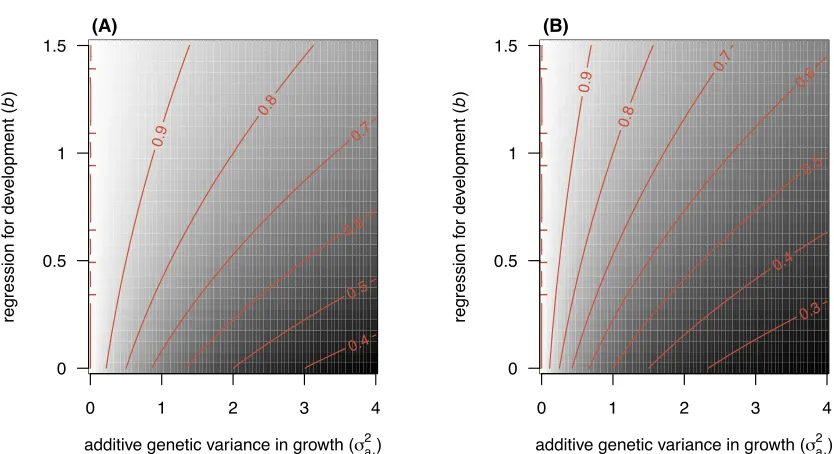
specific conditions. According to equation (12), for parent-o↵spring regression in juveniles to be fully recov-413

ered by a model using a cross-age biometric inheritance function, the phenotypic variance in growth, 2

z A, 414

must be zero. When that is not the case, the proportion of regression recovered decreases with decreasing 415

size-dependent size regression,b(Equation 7, Figure 6A). The same condition holds for the parent-o↵spring 416

regression in adults (Equation 8, Figure 6B). These quite narrow conditions are unlikely to occur in nature. 417

We obtained similar results for the case where covariance in growth exists (Appendix B). Indeed, although 418

IPMs were developed to model dynamic traits, the conditions for which they are guaranteed to recover 419

parent-o↵spring regression, particularly the absence of variance in growth, essentially constrain a dynamic 420

trait to be static. 421

422

Parent-o

↵

spring regression with a constant intercept

423

The preceding analysis shows that regression to the mean prevents the inheritance function from capturing 424

most aspects of covariance between individuals and their descendants. In language typically used to describe 425

properties of IPMs, a cross-age biometric inheritance function does not fully capture the most important 426

ways in which inheritance influences the dynamics of a population through time. Importantly, however, as 427

shown above, the biometric inheritance notion does capture the correct covariance of parents and o↵spring, 428

at least of a static trait (or a model with a single age class). In itself, this may imply that a purely bio-429

metric notion of inheritance can be used, at least in simple cases, to track some important features of a 430

population. Nonetheless, the use of the concept of biometric inheritance that is extensively recommended 431

for IPMs (Coulson et al., 2010; Coulson, 2012; Rees et al., 2014) does not correctly employ the concept. This 432

recommendation is based on two misconceptions about biometric inheritance, both of which lead to failures 433

to characterize even the simplest aspects of phenotype (e.g. the dynamic of mean phenotype). The first mis-434

conception, shown above, is the assumption that theory underlying the biometric relations among kin can be 435

applied to a non-static trait when parents and o↵spring are of di↵erent ages. This includes the assumption 436

that iteration of the purely phenotypic relations of parents and o↵spring across multiple generations can 437

recover biometric relationships among more distant kin, e.g. arbitrary ancestral regressions. The second 438

misconception is that the biometric inheritance concept, and its known relationships to quantitative genetic 439

genetic basis (e.g. an assumption thath2 _{is constant over a period of time) to a trait is commonly assumed}

441

in quantitative genetic studies, and implies that the slope of the parent-o↵spring regression is constant. 442

However, should a trait evolve, changing the mean phenotype, then the intercept of the parent-o↵spring 443

regression necessarily changes. If the intercept is assumed to not change, or a model is constructed where 444

the intercept cannot change, then the dynamic of mean phenotype will be highly restricted. Therefore, even 445

the simplest possible IPM constructed with a typical inheritance function, which has not only a constant 446

slope, but also a constant intercept, will necessarily fail in describing the evolution of mean phenotype. 447

448

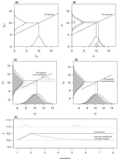
As an example, consider a non-age structured population, with no class structure other than that associated 449

with some focal trait, z. We denote the mean trait value in generation

g

450

Without loss of generality, we assume that during a period of equilibriumz is measured such that its mean 451

is 10. We also assumed thatz is heritable (h2_{= 0.5) but, since there is no selection, no phenotypic change}

452

is observed (Figure 7A). Suppose that the equilibrium is then disrupted and that both sexes experience 453

the same selection, which represents a change in mean phenotype for the first generation ( ¯z0

1) of 1 unit

454

(Figure 7B). The o↵spring on mid-parent regression is thenE[z2] = ↵+h2z1m+z1f

2 , where↵ is the

inter-455

cept and z1m and z1f denote maternal and paternal phenotypes, respectively. An IPM constructed using 456

this regression (appropriately handling the two sexes) yields a mean phenotype in the next generation of 457

¯

z2=R↵+h2

·z_·p1(z)dz=↵+h2_{(¯z1+ ¯z}0

1). The first expression corresponds to the integral that would be

458

solved (typically numerically) by an IPM corresponding to this example, andp1(z) is the probability density 459

function of phenotype after selection but before reproduction in generation 1. The second expression is the 460

analytical solution for this integral, made possible by assuming a linear function. Under the conditions set 461

for this example, this expression would be ¯z2= 5 + 0.5·(10 + 1) = 10.5. This change satisfies the breeder’s 462

equation for the change in mean phenotype across generations ¯zi+1 z¯i=h2 z¯0. The problem arises in the 463

next generation. 464

465

Let us suppose that selection is now relaxed, such that the within-generation change in phenotype due to 466

selection, z¯0

2, is zero. In the absence of selection, drift, immigration and mutation, we expect no change

467

in allele frequencies (Wright, 1937) and therefore no evolution. Consequently, we expect no change in mean 468

phenotype (Figure 7C). In a very simple non-age structured IPM, we would use the current distribution 469

of trait values (

g

and that would correspond to ¯z3 =R↵+h2·z·p2(z)dz=↵+h2(¯z2), which in this case would be 10.25 471

(Figure 7D). In this example, an IPM would predict the trait moving back 0.25 phenotype units, which 472

static biometric inheritance function results in changes in mean phenotype in the absence of selection, drift, 474

mutation and migration. Continuing the analytical iteration of the mean phenotype in this simple IPM, we 475

show that with each subsequent generation (iteration step, in this simple argument), the mean phenotype 476

regresses further toward a value determined by the nature of the static biometric inheritance function (Fig-477

ure 7E). If selection is sustained, then the dynamic of the mean phenotype even in this very simple IPM 478

will be wrong, representing a component associated with the response to selection, and a spurious change 479

due to the misconception of biometric inheritance associated with a parent-o↵spring regression with a fixed 480

intercept. A biometric inheritance function with a constant slope and intercept is inconsistent with evolution. 481

482

Study case: bighorn sheep

483

We used a pedigreed population of bighorn sheep from Ram Mountain, Alberta, Canada (52 N, 115 W) 484

to assess the performance of the development and inheritance functions as implemented in standard IPMs. 485

Both quantitative genetic (e.g. Coltman et al., 2003; Wilson et al., 2005) and IPM analyses (Traill et al., 486

2014) have been conducted for this study system. This isolated population has been the subject of intensive 487

individual-level monitoring since 1971. Sheep are captured and weighed multiple times per year between 488

late May and late September. For detailed information on the study system see Jorgenson et al. (1993), 489

Festa-Bianchet et al. (1996) and Coltman et al. (2003). We analyzed individual age-specific masses adjusted 490

to September 15 (see Martin & Pelletier, 2011; Traill et al., 2014) for 461 ewes captured from 1975 to 2011 491

and aged up to 10 years (2002 ewe-years). We built two statistical models, one reflecting how the ontogenetic 492

development of size and inheritance have been typically modelled in IPMs, and the other corresponding to 493

a possible alternative to estimating these two key functions, a random regression animal model of body size 494

(Kirkpatrick et al., 1990, 1994; Meyer & Hill, 1997; Meyer, 1998; Wilson et al., 2005). We chose random 495

regression because it is widely used to study the genetics of developmental trajectories and it satisfies a 496

number of criteria, namely: (i) it accommodates across-age covariance, over and above that attributable to 497

measured values of focal traits, (ii) it incorporates the known fundamentals of quantitative genetics, (iii) it 498

is economical in terms of the number of parameters that need to be estimated, and (iv) its basic structure is 499

compatible with IPMs. Criteria (i) and (ii) result in random regression analysis providing an approach for 500

characterizing development and inheritance that should be robust to regression to the mean, as imperfectly 501

measured quantities are not used as predictor variables, and as it uses a modern notion of inheritance of 502

quantitative traits. Nonetheless, other options can also avoid regression to the mean, including a formulation 503

though the random regression approach, and potentially other models using quantitative genetic approaches 505

characterizing variation in phenotype and its inheritance, could profitably be integrated into the broader 506

IPM framework, for simplicity we refer to the former approach as “IPM” and to the latter as “RRM”. Both 507

models were fitted in a Bayesian framework, using MCMCglmm (Hadfield, 2010), and di↵use inverse gamma 508

priors for all (co)variance components. 509

510

Standard IPM approach

511

We used a linear model to estimate the development and inheritance functions used in typical IPMs. We 512

modelled observed ewe mass at each age as a function of mass at the previous age, with separate intercepts 513

and slopes for each age. For lambs, we estimated a regression of lamb mass on the mass of their mother two 514

months before conception (previous September). Formally, the model is described as 515

xi,a⇠N(ua+bdeva⇥Iadulti⇥xi,a 1+binh⇥Ilambi⇥mothermassi, ei,a), (13)

where xi,a is the observed mass of individual i at age a, ua age-specific intercepts, bdeva age-specific size

516

slopes andbinhis the inheritance function coefficient. IlambandIadult are indicator variables for lambs and 517

older individuals, respectively. Finally, ea are heterogeneous residuals per age. The estimated fixed e↵ects 518

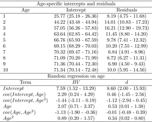
and variance parameters are presented in table 1. 519

520

Random regression of size

521

To model the family of size-at-age functions in bighorn sheep ewes, its genetic basis, and associated pheno-522

typic and genetic covariances of size across age, we fitted a random regression animal model (Kirkpatrick 523

et al., 1990, 1994; Meyer & Hill, 1997; Meyer, 1998; Wilson et al., 2005) of the form 524

xi,a⇠N(µa+f1(di, n1, a) +f2(BVi, n2, a), ei,a), (14)

where xi,a is the mass of individual i at age a and µa are age specific intercepts. f1 and f2 are random 525

regression functions on natural polynomials of order n, for permanent environment e↵ects and additive 526

genetic values, respectively. The permanent environment e↵ect refers to all consistent individual e↵ects other 527

than the additive genetic e↵ect (see Kruuk & Hadfield, 2007). In bothf1 andf2, nwas set to 2, allowing 528

standard deviation-scaled ages to improve convergence. Finally, heterogeneous residuals across ages were 530

estimated (ei,a). d and BV, vectors with individual and pedigree values, respectively, were assumed to 531

follow normal distributions,d⇠N(000, DDD) andBV ⇠N(0, GGG⌦AAA). BothDDD=III 2i, where 2i is the permanent 532

environment e↵ect of individuali, and the additive genetic variance-covariance matrix,GGG, are 3_⇥3 matrices, 533

AAA is the pedigree-derived additive genetic relatedness matrix, and _⌦ denotes a Kronecker product. More 534

information on partitioning phenotypic variance into di↵erent components of variation using pedigrees and 535

the animal model is provided by Lynch & Walsh (1998), Kruuk (2004) and Wilson et al. (2010). To obtain 536

the genetic variance-covariance matrix for the 10 ages, the following equation is used 537

G10 G10

G10= GGG T, (15)

whereG10G10G10is the resulting 10⇥10 genetic matrix,GGGis the 3⇥3 genetic matrix estimated by the model and 538

is a 10⇥3 matrix with the polynomials evaluated at each age (Kirkpatrick et al., 1990; Meyer, 1998). 539

A 10_⇥10 matrix,D10D10D10, for individual e↵ects at the 10 ages can be obtained similarly. The estimated fixed 540

e↵ects and variance parameters are presented in table 2. 541

542

Recovering resemblance within and across-generations

543

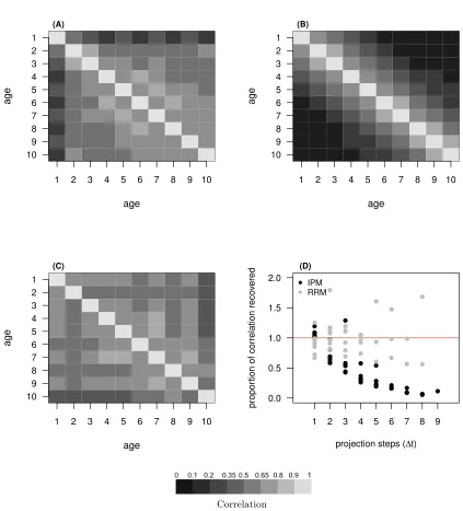
We compare the correlations in mass among ages implied by the development functions typically adopted 544

in IPMs and those derived from a RRM, to the observed phenotypic correlations (Figure 8A-C). We used 545

the path rules, as described for the theoretical models, to obtain the correlation matrix for size at di↵erent 546

ages implied by the IPM approach. There was no need to do the same for the RRM, as these correlations 547

were recovered with equation (15). We also analyze the proportion of correlation recovered for di↵erent gaps 548

between ages (projection steps,

t

tion matrix (Figure 8C) that is much more similar to that observed (Figure 8A) than the correlation matrix 550

implied by the IPM approach (Figure 8B). Across-age correlations are better recovered by the RRM than 551

by the IPM approach (Figure 8D). The proportion of correlation in size among ages recovered by an IPM 552

follows the pattern predicted in figure 2, with high recoveries for a single projection step, and then rapidly 553

decaying to near zero (Figure 8D). As predicted by our theory, typical parameterizations of the development 554

functions severely underestimate similarity of trait values within individuals across ages. 555

556

Second, we show the parent-o↵spring regressions recovered by the RRM and the IPM, and use the “ob-557

on maternal mass for all matching ages, also including random intercepts for mother ID by age, year and 559

cohort, as well as heterogeneous residuals by age. The cross-age biometric inheritance function implemented 560

in IPMs recovers parent-o↵spring regression for lambs (age 1), but for older ages most similarity between 561

parents and o↵spring is missed (Figure 9). In contrast, the patterns of parent-o↵spring similarity recovered 562

by the RRM are of the observed order of magnitude throughout most of the life cycle (Figure 9). 563

564

Discussion

565

We have shown analytically that IPMs, as typically implemented, will generally, and often severely, under-566

estimate quantities that are critical to evolutionary inference. Both our theoretical results and our empirical 567

example show that phenotypic covariances within and across individuals can be e↵ectively zero in these mod-568

els, due purely to artifacts of their construction. Additionally, the static nature of the inheritance function 569

(parent-o↵spring regressions with fixed intercept) artificially reverses any response to selection. Consequen-570

tially, IPMs, as typically constructed, will inevitably suggest that evolution is not an important aspect of 571

the dynamics of traits over time. We suggest, and demonstrate empirically, alternative approaches that 572

could be used to characterize some key functions in IPMs. IPMs in principle are extremely useful and highly 573

flexible, and their original conceptualization (Easterling et al., 2000; Ellner & Rees, 2006) should be broadly 574

compatible with a variety of alternative ways of characterizing variation in growth and inheritance. 575

576

The main reason why development functions in IPMs fail to recover within-generation covariances of traits is 577

regression to the mean. This problem is well-understood in evolutionary and ecological studies (e.g. Kelly & 578

Price, 2005). In IPMs, this problem is particularly severe because the multiple age-specific projection steps 579

compound the e↵ect of measurement error to reduce covariance among predictor and response variables. Con-580

sequently, covariance between non-adjacent ages, which can be substantial (Figure 8A, Wilson et al., 2005), 581

is severely underestimated (Figure 8B), even when measurement error is relatively small (Equations 1 and 2). 582

583

The failure of biometric inheritance functions to predict phenotypic similarity among relatives is partially 584

also a direct manifestation of regression to the mean. Indeed, it is the canonical manifestation of regression 585

to the mean – coined in exactly this context by Galton (1886). What we now understand is that Mendelian 586

factors are inherited, and that, in terms of statistical mechanics of quantitative genetics, environmental 587

variation can be regarded as measurement error obscuring the influence of breeding values. Any model of 588

in quantitative traits (Fisher, 1918, 1930; Wright, 1922, 1931) cannot be expected to suffice for even the 590

most basic evolutionary predictions. Another issue arises from assuming that the biometric inheritance 591

function is constant. Whenever the mean phenotype changes, the intercept of the parent-o↵spring regression 592

necessarily changes as well. To presume that the intercept of the parent-o↵spring regression is constant 593

across generations constrains the mean phenotype to be able to respond only transiently to selection, as we 594

show by analytically iterating the mean phenotype in a simple IPM model structure (Figure 7D). We reit-595

erate that our criticism of a constant inheritance function is not a criticism of models assuming a constant 596

heritability, whether that heritability is modelled using a genetical (i.e. using constant 2

a

z) or a 597

biometric approach (i.e. using a parent-o↵spring regression with a constant slope). Rather, the key point 598

is that the mean phenotype cannot evolve in a model where a parent-o↵spring regression has a fixed intercept. 599

600

In our theoretical models, we use simple but general development and inheritance functions that are specif-601

ically designed to isolate these two fundamental processes from each other. In practice, however, the un-602

desirable behaviours that we have modelled separately will interact. Importantly, in iteroparous organisms, 603

where multiple episodes of reproduction occur over the lifetime, regression to the mean in development 604

functions will further obscure relationships between parents and o↵spring, with increasing e↵ects as parents 605

age (Chevin, 2015). Additionally, biased estimates of covariance of parents and o↵spring are compounded 606

across multiple generations. The underestimation of similarity between parents and o↵spring will be com-607

pounded at each generation, leading to increasingly severe undervaluation of the relevance of relationships 608

among more distant relatives to the evolutionary process. This interaction is very evident in the empirical 609

example we present. Parent-o↵spring regressions recovered with the development and inheritance functions 610

generally used in IPMs (Figure 9) could not be predicted by the two-age theoretical model presented here, 611

and specifically by equation (11). 612

613

IPMs with typical cross-age biometric inheritance functions have been recommended for studying evolution-614

ary responses to selection (Coulson et al., 2010; Coulson, 2012; Rees et al., 2014). Some studies applying this 615

approach have concluded that non-evolutionary changes in trait distributions are the major contributors to 616

temporal changes in phenotype (Ozgul et al., 2010; Traill et al., 2014). Our theoretical findings do not indi-617

cate that these conclusions are wrong. Rather, we demonstrate that these are the conclusions that this kind 618

of model must inevitably generate when applied to any system, regardless of whether evolutionary change 619

is important or not. Since typical parameterizations of IPMs neglect the vast majority of similarity between 620

parents and o↵spring, they cannot attribute phenotypic change to evolution. Concern about how IPMs model 621

& Langangen, 2015; van Benthem et al., 2016). Particularly, Chevin (2015) identified some issues addressed 623

in this paper, presenting insightful numerical examples that illuminate the main concern with the cross-age 624

structure of the inheritance function. Besides our analytical demonstrations, and the numerical examples 625

made available by Chevin (2015), we also provide an empirical example, using random regression analysis 626

to address the issues presented here. The random regression model provided substantial improvement in 627

recovering both correlations across ages within a generation (Figure 8D), and parent-o↵spring regressions 628

reflecting how breeding values are transmitted over generations (Figure 9). 629

630

Vindenes & Langangen (2015) discuss joint models of static traits (constant through life) and dynamic traits 631

(such as those typically handled in IPMs) in the general IPM framework. They suggest that incorporation 632

of static traits could solve some of the problems that had begun to be acknowledged about evolutionary 633

inference with IPMs (Hedrick et al., 2014; Chevin, 2015). The authors propose that the static trait, birth 634

mass in their example, could be modelled as influencing mass at all other ages and demographic rates, which 635

would allow covariances among birth mass and older ages to be well recovered. In a sense, using random 636

regression animal models as we suggest treats breeding values (as opposed to some realized phenotypic value) 637

as a static trait, but critically also models the inheritance of breeding values, not as some observed function, 638

but according to the principles of quantitative genetics. It is noteworthy to mention that a genetic notion 639

of trait transmission has already been implemented into an IPM for a single Mendelian locus (Coulson 640

et al., 2011). The authors constructed an IPM that describes the dynamics of body mass and a biallelic gene 641

determining coat color in wolves (Canis lupus). In contrast to biometric IPMs of quantitative traits, Coulson 642

et al. (2011) conclude that the genetic variance within the study population is enough for natural selection 643

to cause evolution. In fact, it is in principle relatively straightforward to implement an IPM that uses the 644

basic principles of inheritance of polygenic quantitative traits to define inheritance functions of breeding 645

values; such exercises have indeed begun for a single trait (Childs et al., 2016). It is easy to conceive of 646

multivariate extensions of such inheritance functions (based on multivariate versions of equations 3 and 647

4), whereby one could treat age-specific sizes as di↵erent characters, and estimate genetic variances and 648

covariances from data. Nonetheless, a great deal of work is still required. For long-lived organisms, genetic 649

covariance matrices of age-specific traits would be very challenging to estimate with useful precision (Wilson 650

et al., 2010). Furthermore, the dimensionality of resulting phenotypes would overwhelm typical strategies 651

for implementing IPMs (Coulson et al., 2010; Rees et al., 2014; Merow et al., 2014). In practice, a key 652

challenge, but a surmountable one, will be to develop sufficiently flexible, low-dimensional characterizations 653

of the genetic basis of development for practical estimation and subsequent modelling. The function-valued 654

possibility. Other approaches could possibly be even more useful; for example, uses of various autocorrelation 656

functions (Pletcher & Geyer, 1999; Hadfield et al., 2013), or factor-analytic mixed model (de los Campos & 657

Gianola, 2007; Meyer, 2009; Walling et al., 2014). 658

Summary

659

We have shown analytically and using and empirical example that standard implementations of integral 660

projection models will generally severely underestimate the likelihood of evolutionary change. IPMs to date 661

have been constructed using characterizations of development and inheritance that would not stand up to 662

scrutiny in studies focusing on development and inheritance. It is not surprising that more complex models 663

built on such functions behave poorly. In fact, insofar as the ability of IPMs to track the full joint distribution 664

of phenotype has been suggested as their main quality for ecological inference, the problems that preclude 665

their typical use for evolutionary inference should be of equal concern to ecologists. Importantly, we have 666

suggested ways in which more nuanced models of development, and a modern understanding of inheritance, 667

can be incorporated into the general IPM approach. A great deal more work is required before IPMs based 668

on adequate models of development and inheritance will be field-ready. As a next step, careful studies of the 669

performance of di↵erent approaches for characterizing the genetic basis of developmental trajectories, with 670

particular focus on approaches that could be incorporated into an IPM framework, are needed. 671

Acknowledgments

672

We thank Jarrod Hadfield, Loeske Kruuk, Luis-Miguel Chevin, Josephine Pemberton, Graeme Ruxton, Jean-673

Michel Gaillard, Sandra Hamel, and two anonymous reviewers for valuable comments and discussions. We 674

are also very grateful to all those who worked on the bighorn program over decades. The bighorn research 675

is supported by the Government of Alberta, the Universit´e de Sherbrooke and an Alberta Conservation 676

Association Challenge Grant in Biodiversity, NSERC Discovery Grants to D. Coltman, M. Festa-Bianchet 677

and F. Pelletier and the Canada Research Chair in Evolutionary Demography and Conservation. M. B. 678

Morrissey is supported by a University Research Fellowship from the Royal Society (London). M. J. Janeiro 679

is supported by a PhD scholarship (SFRH/BD/96078/2013) funded by the Funda¸c˜ao para a Ciˆencia e 680