Advances in Visibility Modelling in Urban Environments to Support Location Based Services

(1)

Advances in Visibility Modelling in

Urban Environments to support

Location Based Services

______________________________________________________________

A thesis

submitted in partial fulfilment of the requirements for the Degree

of

Doctor of Philosophy in the

University of Canterbury by

Phil Bartie

______________________________________________________________

University of Canterbury Christchurch, New Zealand

(2)

ii

Acknowledgements

There are a large number of people to thank! Of course firstly Simon, Femke, and Steven for your expert advice, invaluable guidance, constant encouragement and for taking me on. Also to Clive Sabel, Burn Hockey and Mark Billinghurst for getting me started.

Mark Kumler and Eliseo Clementini for agreeing to co-author papers with me from out of the blue. Peter Woodrow from the City Council for granting access to the Christchurch LiDAR data. The University of Canterbury for funding, and the Geospatial Research Centre staff and fellow students for making spatial research so much fun. Special mention must go to Dan, Meghan, Matt and Welshy for our GIS conversations over a cuppa, also Dave, Offy and Eli for chats about coding over a beer, and William Mackaness for ongoing spatial guidance from afar.

(3)

iii

Abstract

(9)

2

Chapter 1:

Introduction

1.1 Introduction

The “information age” is a time of unequalled access to knowledge, with capabilities to transfer information more freely than ever before. However “information overload” can become a problem as the quantity of data increases, requiring better solutions to sustain search efficiency and maintain information relevance (Morville 2005). One strategy to improve search effectiveness is to automatically include location as a criterion, thereby limiting results by spatial significance. Location awareness is particularly relevant for the post-desktop era of ubiquitous computing (Weiser 1993, Weiser et al. 1999), especially for mobile devices referred to as Location Based Services (LBS), a good account of which can be found in Jiang and Yao (2006).

Location is most typically introduced as a search parameter based on proximity, filtering the results based on an arbitrary distance measured in Euclidean or network space (Mountain and MacFarlane 2007). However people describe and explore space with a heavy emphasis on the visual senses, something under-used as a search parameter within LBSs (May et al. 2005). In part this has been due to the lack of useful data but recent advances in data capture, such as Light Detection and Ranging (LiDAR), provide an economically viable way to build digital city models leading the way to the inclusion of visibility analysis in a wider range of urban applications (Palmer and Shan 2002, Rottensteiner and Briese 2002, Bartie and Mackaness 2006).

This thesis develops visibility modelling and its inclusion in a range of novel functions for use in urban LBS with the goal of supporting new types of user interaction. This begins with the development of a new model for filtering and quantifying the visibility of features of interest (FOI) taking into account views through and under vegetation canopy. A model able to store the relationship for the results from an egocentric perspective is developed, matching the user‟s view, providing the foundation for describing visible features using projective spatial relationship terms, such as “in front of” and “left of” (Freeman 1975, Clementini and Billen 2006, Clementini 2009). This can be combined with other descriptive attributes, such as building colour, to form useful referring expressions (Dale and Reiter 1995). These referring expressions will be required in advancing speech based user interfaces, which are considered to be a beneficial addition to future LBS devices as they allow the user to maintain focus on their surroundings, operating eyes-free and hands-free (Goose et al. 2003, Sharma et al. 2003, Howell

et al. 2005, Bartie and Mackaness 2006).

(10)

3 1. Develop a visual exposure model for use in an urban LBS, which delivers a range of

new metrics suitable to quantify the visibility of nominated features of interest.

2. Accommodate under canopy and through canopy views of features of interest within the visual exposure model.

3. Express relationships between visible features from the user‟s viewpoint using an egocentric projective model of space, with support for storage and querying.

4. Determine the most suitable referring expression to describe a visible item to the LBS user, using visual attributes (e.g. size, colour, position).

1.2 Thesis Structure

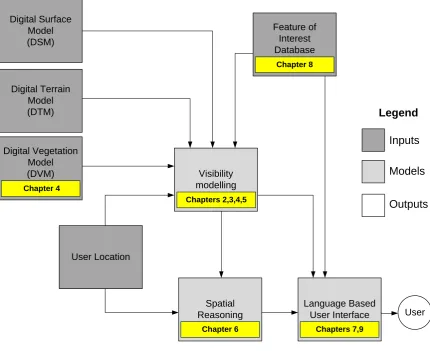
The thesis begins by examining the wider context of LBS with a review of current positioning solutions and mobile user interfaces. A new visual exposure model is developed in Chapters 2 and 3, suited to urban environments, able to generate a number of metrics for Features of Interest (FOI) in a scene. The term FOI is used throughout, rather than just the usual Points of Interest (POI), as consideration is given to regions of visibility corresponding to urban objects (e.g. statues, buildings). The advances made include measuring visible façade areas, with detailed information on which foreground features block the view leading to the introduction of a viewing clearness metric. The impact of vegetation within the visual exposure model is addressed in Chapter 4, such that partial through canopy and under canopy views are modelled. The use of the model as part of a navigation task is explored in Chapter 5, such that a motorist is pre-informed of blind corners and good overtaking opportunities along a defined route.

As speech recognition improves so speech based user interfaces will become a more viable interaction method on mobile devices. The need to verbalise spatial information in a format that can be easily comprehended raises the topic of how referring expressions may be generated for visible entities based on their appearance from the user‟s perspective. Part of the issue is in how objects are described in egocentric projective space (Chapter 6), but also in how descriptions may be formed using the most salient visual attributes (Chapters 7 & 9). Both of these concepts are discussed, and the issue of how building colour information may be collected is also examined in Chapter 8. Here a new approach is demonstrated to combine computer vision techniques with spatial analysis to automate the collection of house and boundary wall colours, filtering out foreground objects. This information is used in conjunction with other datasets to form useful descriptions of the features in view, such that a LBS user‟s attention could be directed to a target feature.

(11)

4 Digital Surface

Model (DSM)

Digital Terrain Model (DTM)

Digital Vegetation Model (DVM)

User Location

Feature of Interest Database

Visibility modelling

Spatial Reasoning

Language Based User Interface

Inputs

Models

Outputs

Legend

Chapter 6 Chapters 7,9

Chapter 8

Chapters 2,3,4,5 Chapter 4

[image:11.595.99.530.131.482.2]

User

Figure 1.1: Schematic of Information Flow for a LBS with Corresponding Thesis Chapters

1.3 Academic Papers

(12)

5

Objective 1) Develop a visual exposure model for use in an urban LBS, which delivers a range of new metrics suitable to quantify the visibility of nominated features of interest.

 Chapter 2) Bartie, P. J., Mills, S. & Kingham, S., 2008. An egocentric urban viewshed: a method for landmark visibility mapping for pedestrian location based services. In Moore, A. & Drecki, I. (eds.) Geospatial Vision - New Dimensions in Cartography. New Zealand, Springer, 61-85.

 Chapter 3) Bartie, P. J., Reitsma, F., Kingham, S. & Mills, S., 2010. Advancing visibility modelling algorithms for urban environments. Computers Environment and Urban Systems, 34(6), 518-531.

Objective 2) Accommodate under canopy and through canopy views of features of interest within the visual exposure model.

 Chapter 4) Bartie, P., Reitsma, F., Kingham, S. & Mills, S., 2011. Incorporating vegetation into visual exposure modelling in urban environments International Journal of Geographical Information Science, 5 (5), 851-868.

 Chapter 5) Bartie, P. J. & Kumler, M. P., 2010. Route ahead visibility mapping: a method to model how far ahead a motorist may view a designated route. Journal of Maps, April 2010, 84-95.

Objective 3) Express relationships between visible features from the user’s viewpoint using an egocentric projective model of space, with support for storage and querying.

(13)

6

Objective 4) Determine the most suitable referring expression to describe a visible item to the LBS user, using visual attributes (e.g. size, colour, position).

 Chapter 7) Bartie, P., Reitsma, F. ,Clementini, E., & Kingham, S, 2011. Referring expressions in location based services: the case of the “opposite” relation, in Semantic Enrichment of 3D city models for sustainable urban development, SECOGIS 2011, Springer-Verlag, Brussels, Belgium.

 Chapter 8) Bartie, P., Mills, S. & Reitsma, F., 2011. Building Colour Terms: a combined GIS and stereo vision approach to identifying building pixels in images to determine appropriate colour terms, Journal of Spatial Information Science, 2(2011), 59-83.

 Chapter 9) Bartie, P., Reitsma, F., & Kingham, S., (yet to submit). Referring

expressions in urban environments: generating and comprehending expressions using Bertin‟s visual variables. Journal of Location Based Services (to be submitted).

1.4 Additional Contributions by the Candidate

It should also be noted that during the PhD programme the candidate published two additional papers. The first is included in Appendix A, and describes a technique to use a smartphone to capture video and audio data with the corresponding time and location details, intended for use in conjunction with synchronised environmental sensors. The media is able to assist researchers in the data analysis stage by providing context from the time of collection, which can help to understand variations in the environmental data caused by temporal events, such as an increase in air pollution cause by a passing bus. The second paper relates to the presentation of thermal imaging on a LiDAR sourced city model.

 Bartie, P., & Kingham, S. (2010). Media mapping: using georeferenced images and audio to provide supporting information for the analysis of environmental sensor datasets. The Journal of the Open Source Geospatial Foundation, 8.

(14)

7

1.5 Background

Developments in a number of technologies have created opportunities for new kinds of interaction with computers, and digital data. These include more powerful mobile computing platforms, better location solutions across a wider range of environments, improved user interfaces, and access to data through faster network connections. As a result a new breed of mobile computing exists where users can query their environment in situ. The following summarises some of the key research in these areas providing additional background material to that in each of the thesis chapters.

1.5.1 Location Based Services

LBSs are location-aware and context-aware applications running on mobile devices capable of providing information to the user on their surroundings (Jiang and Yao 2006) the majority of which provide way-finding assistance (Douglas et al. 2006).

Cyberguide (Long et al. 1996) was a LBS pioneer, able to calculate its location indoors using infrared beacons and outdoors using the Global Positioning System (GPS), providing location customised information to tourists. The system demonstrated that mobile computing was able to usefully adapt information delivery based on location and place histories, offering an alternative to a human tour guide.

A wide variety of location aware applications have been developed since, including GUIDE a virtual guidebook (Davies et al. 1999, Cheverst et al. 2000), EASYGO for public transport information (Gartner et al. 2007), GEONOTES for attributing space using virtual tags (Espinoza

et al. 2001), urban gaming (Benford et al. 2006), friend finding (Strassman and Collier 2004, Neer 2011), and way-finding applications (May et al. 2003, May et al. 2005, Google 2006).

The uptake of LBS by the population has been fairly slow, which can be partially attributed to poor user experiences, a lack of service dependability, and a lack of perceived ownership benefits (Chincholle et al. 2002). Furthermore many potential users are concerned about issues of privacy (Duckham and Kulik 2006) and security (Cahill et al. 2003). However driven by the inclusion of GPS in smartphones and the availability of free, or very cheap, applications it appears that LBS popularity is on the rise (Williams 2009, Kim 2011). There are also initiatives such as OpenLS (Zipf 2004, OGC 2008), which aim to standardise access protocols to spatial data services and content repositories, facilitating wider adoption across a growing range of devices.

(15)

8 fairly high location resolution and a digital compass to track device orientation, and are sometimes referred to using the term Mobile Spatial Interaction (Fröhlich et al. 2009).

1.5.2 Positioning techniques

A LBS should be able to automatically and continuously determine the user‟s position so that relevant information may be retrieved and presented. Global Navigation Satellite Systems (GNSS), such as GPS, have become a widely adopted solution for doing this as they offer global coverage with minimal operating and maintenance costs for the end user; a full operational overview can be found in Kaplan and Hegaty (2006). Despite the widespread popularity of GPS it has an “Achilles heel” (Raper et al. 2007), struggling to operate in “urban canyons” where the direct lines of sight to the GPS satellites are occluded, and signals reach the receiver after being reflected from nearby surfaces, known as multipath signals. The situation is worse for pedestrians positioned on the pavement, close to tall buildings, as satellites are occluded to a greater extent than for motorists positioned near the centre of the street.

There are several strategies to improve GPS performance, two of the most successful currently implemented are the Satellite-Based Augmentation System (SBAS) (Ott et al. 2005) and Assisted-GPS (A-GPS) (Cho 2004). SBAS is a satellite based Differential-GPS (DGPS) system consisting of a separate series of satellites and ground stations which transmit GPS correction details, including data on signal delays due to atmospheric effects and clock drift, typically improving location accuracy for equipped devices to 3 metre accuracy (Garmin 2011). SBAS is known as WAAS in USA, EGNOS in Europe, and MSAS in Japan, however Australia and New Zealand are not currently supported by such a system.

A-GPS aims to decrease the time to first location fix by using a networked service to provide the mobile client with supporting information on relevant satellite orbital data, ionospheric conditions, and assistance in matching fragments of GPS signal received. The benefits are a decrease in the time taken to calculate a location, and the ability to decode weaker signals, but not an improvement in location accuracy. It is available world-wide but requires that the mobile device has an internet connection to download the relevant supplementary data.

(16)

9 Position robustness may also be improved by supplementing GNSS solutions with extra sensors known as Inertial Measurement Units (IMUs) able to supply relative motion changes. These can be placed on the user‟s foot to exploit human walking kinematics and therefore to estimate the user‟s position in between GNSS updates (Radoczky 2007). An IMU incorporates a number of sensors which record movement direction and magnitude, including a combination of accelerometers able to measure movement forces in 3 dimensions, gyroscopes able to track direction changes, and barometers to measure elevation changes, which is particularly useful inside buildings for floor level estimation.

IMUs are able to assist GNSS in challenging environments (e.g. indoors, urban canyons) but without GNSS updates the positional errors accumulate over time and positional drift occurs. The rate of this drift varies depending on the quality of the sensors in the IMU, but can be improved by monitoring the user‟s steps and performing zero velocity updates. These are when the IMU is known to be static as the user‟s foot is placed on the ground, and therefore the sensors may be re-calibrated (Mezentsev et al. 2005). The GNSS and IMU sensor inputs are integrated into a single best estimate of location using a Kalman filter (Yang et al. 2008), which has demonstrated to be effective in a number of projects (Godha et al. 2005, Ott et al. 2005).

There are a number of other emerging technologies in various stages of development which could one day provide a high resolution urban positioning solution. For example terrestrial radio waves fill urban environments, and Robust Surface Navigation (RNS) (Hodge 2007) relies on using these “signals of opportunity” to calculate the user‟s location. Signals suitable for this include FM Radio (Krumm et al. 2003), AM signals (McEllroy et al. 2007), cellular phone network signals (Zhou et al. 2005, Chen et al. 2006) and other shorter range signals such as Wi-Fi (Hightower et al. 2005).

Dense networks of Wi-Fi base stations found in cities provide a useful fast positioning solution. Wi-Fi equipped mobile platforms permit developers to access signal strength information from all the surrounding access points, meaning position triangulation is possible. Trials have shown that a median location accuracy of 30m can be achieved in urban areas (LaMarca et al. 2005). This method requires a database of the physical locations of each Wi-Fi base station with its corresponding unique Media Access Control (MAC) address. There are a number of open source databases, maintained by community volunteers, which hold this information, such as Placelab (LaMarca et al. 2005). However Wi-Fi signals may only cover a small proportion of the city, and as the base stations are not controlled by a single operator any unit may be moved or turned off without prior notice. A number of commercial companies have begun to offer applications which combine the location benefits from cell tower, Wi-Fi and GPS positioning solutions, such as Skyhook (Skyhook 2008).

(17)

10 image to a server which geometrically straightens it for comparison against a database of images from known locations. Typically the key points identified in each image include corners of window frames or doors, which change infrequently. The result is that the user‟s orientation and location can be calculated, usually to within one metre (Randerson 2004). However this technique requires considerable computational power on the server side and frequent image database updates. A manual equivalent exists whereby the user specifies which landmarks are visible, and the mobile device calculates the possible locations that they may be (Kray and Kortuem 2004). A negative aspect of both of these methods is that the system latency renders the techniques unsuitable for continuous tracking.

This tracking issue is also of interest in robotics research, referred to by the acronym SLAM which means Simultaneous Localisation and Mapping. Until recently expensive sensor arrays which included laser and IMUs were required to track robot movements over great distances, but new research has shown that a single digital camera can be used to perform localisation over a 2.5km walk (Botterill et al. 2010). Developments such as these should lead to sustained sub-metre accurate positioning for LBS in urban environments in the near future.

1.5.3 User Interfaces

Interface design must put the user centre stage and consider not only the task requirements but also the environment in which the user and computer connect (Worboys 2001). A very successful interface is one in which the user is not aware of its existence (Weiser 1994), or may only require continuous partial attention rather than be totally engaging (Weiser and Brown 1996). A variety of interfaces, reviewed below, can support this spectrum of interaction.

Graphical user interfaces in mobile devices must convey essential information via limited screen space in difficult environmental conditions (e.g. bright sunlight) and use input methods suitable while moving (Dillemuth 2005). LBSs are able to overcome screen size issues to some extent by carrying out map panning, rotation, and zooming automatically based on user context and location (Frank et al. 2004), and by presenting simplified representations of the surrounding spatial information using a sketch map approach (Richter et al. 2008, Schmid et al. 2010). However graphical user interfaces remain a distraction, requiring the user to refocus attention away from their surroundings.

It has been shown that users are able to carry out multiple tasks more easily if they are using a number of sensory modalities (Allport et al. 1972). One way to attract attention at a specific time is to use haptic interfaces, which make use of the sense of touch. Research has shown that it is possible to guide someone using an array of vibration devices mounted in a vest (Ertan et al.

(18)

11 take place by tapping the device, measured by internal accelerometers, for example to repeat an audio instruction.

A fuller interaction experience is possible using a speech based interface, which is particularly suited to LBS as it offers discreet hands-free and eyes-free use, enabling the user to keep focussed on their environment while receiving (speech synthesis) and giving instructions (speech recognition).

Speech recognition accuracy is dependent on a number of factors including system training and background noise. Noise cancelling microphones are able to assist to some degree, but in many cases speech recognition performs best when limited to a small vocabulary of command words. Demonstrations of speech interfaces for information retrieval can be found in a variety of fields, including emergency response centres, database querying, and searching technical manuals (Goose et al. 2003, Sharma et al. 2003, Du and Crestani 2004). A number of the advantages and disadvantages of speech user interfaces are given in Table 1-1.

Table 1-1: Advantages and Disadvantages of Speech User Interfaces for LBS

Advantages

 Low power consumption compared to LCD screen

 Natural conversational communication

 No distraction from viewing the surroundings (hands free, eyes free)

 Accessible in rain without risk of damage to device

 Accessible to visually impaired people

 Familiarity with the interface hardware, lower learning curve

 Lightweight hardware (headphones, microphone), inexpensive – unlike head mounted displays

 Compact, yet without the constraints of limited screen area and map design

 Secure and discreet – the user may not want to be seen looking at maps or appearing lost

Disadvantages

 Speech recognition errors in noisy streets

 User‟s accent and speed of speaking affects accuracy of voice recognition (system coaching required)

 Does not allow a user to browse the information

 Confusion of target identification and selection in crowded regions

 Cannot be used by hearing impaired

For LBSs to support natural interactions through speech interfaces, leading to more intelligent services, there is a requirement to more closely mimic what a co-located human would communicate based on a shared experience of the surrounding space (Winter and Wu 2009). This includes the ability to refer to surrounding features, and model which items are in view. The next section gives a brief overview of visibility modelling, and its use to establish which features can be observed.

1.5.4 Visibility modelling

(19)

12 topography or building height. Recently 3D isovist modelling has become a possibility by accessing city elevation models which include the urban form (Morello and Ratti 2009).

In rural regions viewsheds are used to determine what is visible from a vantage point by calculating which cells of an elevation model are visible to an observer (Tandy 1967, Lynch 1976), using a line of sight algorithm (Fisher 1993). Elevation data may be stored in rasters or Triangular Irregular Networks (De Floriani and Magillo 1994, De Floriani et al. 1997), and uncertainty may be reflected in the results (Fisher 1994b, Fisher 1995). They have been used in a wide range of applications including finding the most hidden route or those with the best views (Lee and Stucky 1998), studying the visual impact of wind farms (Kidner et al. 1999), and in landscape planning (Fisher 1995). Performance has also received a lot of attention as processing can be computationally intensive, especially across high resolution elevation surfaces (De Floriani et al. 2000, Rana and Morley 2002, Rana 2003, Ying et al. 2006).

The results from viewshed analysis describes “vista space” (Montello 1993), that is the space which can be seen from a static location with only movements of the observer‟s head. Figure 1.2 illustrates its fragmented nature in comparison to Euclidean space and network space.

Network Space

Euclidean Space Vista Space

Observer

Figure 1.2: Spatial filter examples: Euclidean space (200m radius),

(20)

13 Vista space is relevant to a LBS user as it defines the current surroundings, through the objects which are visible, and may be included as a filtering method. It is also appropriate for Mobile AR applications which currently filter information using keyword and proximity leading to screen cluttered with labels referring to items out of sight. This will become more of a problem as the quantity of georeferenced data increases, particularly as crowd sourced volunteered information becomes more commonplace (Black and Coast 2007, Goodchild 2007). The introduction of a visibility model to determine which items are currently in view would allow information to be filtered in accordance with the user‟s real world experience, improve the user experience, and pave the way for new user interface interactions. There are only a few examples of visibility filtering in LBS (Beeharee and Steed 2005, Bartie and Mackaness 2006, Maierhofer

et al. 2007, Carswell et al. 2010). These studies have found visibility to be a useful egocentric filter, but have failed to use the results to describe object visibility in any great detail.

1.6 Contribution of Thesis

This thesis contributes to two main areas of LBS research. These are the advancement of visual exposure modelling in urban regions, and the preparation of information for delivery through a speech interface.

The advancements in visual exposure modelling provide facilities to describe FOIs according to a range of new metrics in urban environment using a high resolution city model (Chapters 2,3). In addition modelling the line of sight through vegetation canopy is addressed by combining a DSM, a DTM and multiband imagery (Chapter 4). While vegetation has been included in visibility modelling to some degree before (Dean 1997, Llobera 2007a), its effect on visual exposure has not previously been researched. In addition the raster vegetation model introduced here can accommodate high resolution density variations across the canopy

Information delivery through a speech interface requires translation into natural language phrases. To assist the user relationships between visible objects are referred to using projective spatial relations, matching the user‟s viewpoint. Chapter 6 presents a new projective model which combines and extends existing models allowing for projective relationships between buildings to be serialised for storage and querying purposes. Chapters 7 and 9 deal with referring expressions, and how rare or unique visual characteristics can be used to disambiguate items in view. In support of this Chapter 8 develops an automated technique to collect colour information terms from building façades by filtering out foreground objects using a combined computer vision and GIS approach. This information can be included in a building‟s description when forming the referring expressions.

(21)

14 navigation application for estimating how far along a route a driver can see, thereby giving advanced warning of sections with limited visibility or good overtaking opportunities. Chapter 7 shows that a simple concept such as “spatially opposite” relies on a mutual visibility between two reference objects and a common central feature.

(22)

15

Chapter 2:

An Egocentric Urban Viewshed:

A Method for Landmark Visibility Mapping for Pedestrian

Location Based Services

2.1 Summary

A variety of information can be provided to pedestrians using location based services in support of tasks such as way-finding. Typically current location aware systems use proximity to filter databases for contextual information. We show that a filter based on the visibility of features is a useful additional capability made possible through the use of digital surface models. A number of visibility metrics are suggested for adoption by a location based service, to provide quantitative visibility information so that items of interest may be ranked according to a meaningful priority. Real world experiences validate the usefulness of these metrics, and a number of improvements are suggested.

2.2 Visibility Modelling and Pedestrian Navigation

There is a growing interest in the development of location based services (LBS) in support of pedestrian activities, both rural and urban (Jiang and Yao 2006). The research presented in this chapter is in anticipation of devices able to support natural pedestrian way-finding and navigation in an urban context. It is argued that the requirements for pedestrian navigation are quite different from that of vehicle navigation. While junctions form a key navigation component for motorists, pedestrians more often use landmarks as cues (Millonig and Schechtner 2007). The urban environment is defined by these landmarks, their organisation, and interrelationships (Fisher-Gewirtzman and Wagner 2003) and there is a strong linkage between what a pedestrian can see and how they comprehend a city. We therefore argue that integrating the capability to use landmark visibility information in a navigational device for urban pedestrian use, requires „egocentric visibility modelling‟.

(23)

16 surrogate in military exercises (Baer et al. 2005), and in examining spatial openness in built environments (Fisher-Gewirtzman and Wagner 2003).

Visibility studies within GIS require access to a digital terrain dataset for the area of interest. These are usually raster grid datasets, considered to be 2.5 dimensional, recording a single elevation value (z) for any location (x,y). In general terms these are known as Digital Elevation Models (DEM), but may be more specifically referred to as Digital Terrain Models (DTM) if they reflect the elevation values of the bare earth, or Digital Surface Models (DSM) if they capture building and vegetation elevations.

There have been numerous previous studies on urban visibility, these have tended to use the 2 dimensional boundary of buildings to calculate isovists (Tandy 1967, Benedikt 1979, Turner et al. 2001). To more closely model urban visibility it is necessary to source a DSM at high resolution, such that building and vegetation profiles are captured accurately. Light Detection and Ranging (LiDAR) remote data capture techniques have been shown to be suitable for this in urban studies (Palmer and Shan 2002, Rottensteiner and Briese 2002), and are considered superior for LOS calculations than using community contributed 3D models of inconsistent and questionable accuracy, such as with the Google 3D Warehouse.

This chapter discusses visibility modelling techniques, and presents a number of additional metrics that will allow future location based services to report landmark information in a more intuitive manner, facilitating the exploration of the city. The chapter draws attention to a number of relevant areas of visibility research, including cumulative visibility. It then explains the line-of-sight algorithm used in this research, and a supporting database architecture to model Features of Interest (FOI). Finally the method is demonstrated in a real world situation.

2.3 Visibility Analysis

If every terrain cell in a line-of-sight path is considered between an observer and target it is referred to as the „golden case‟ (Rana and Morley 2002). Although providing the most accurate results from a terrain model this method is computationally expensive, and therefore much of the previous research has focussed on techniques to reduce the number of calculations by considering only visually important cells. Examples of this include using Triangulated Irregular Networks (TINs) (De Floriani and Magillo 1994), or filtering based on topographic features (Rana and Morley 2002). These essentially look to simplify the terrain complexity, or reduce the number of observer-target pairs considered in viewshed generation.

(24)

17 study region, meaning future users only require a simple lookup to return the stored viewshed result. The computational cost of producing a CID is very high, being an O(n2) calculation, therefore parallel or grid processing techniques are often used (Llobera et al. 2004).

By storing the complete set of viewsheds a number of additional attributes are available for analysis, such as the Cumulative Visibility (Wheatley 1995), or Visual Magnitude (Llobera 2003). These depict the total number of times a cell can be viewed from elsewhere, indicating highly visible regions. Topographically prominent areas such as ridges and peaks often feature highly, however visually prominent landscapes may not necessarily be topographically prominent, such as the high intervisibility which occurs in valleys (Llobera 2003).

2.3.1 The Urban Cumulative Viewshed

In the context of rural DTMs, peaks and ridgelines form important spaces which act as barriers, and occupiable vantage points. In urban DSMs these ridgelines correlate to building roofs, and are not generally occupiable. This has a number of implications with regard to previous research focussed on reducing observer-target pairs, which consider ridgelines to be significant vantage points (e.g. Rana and Morley 2002). To faithfully replicate the situation in urban space, a cumulative visibility map must be based on a DSM and restrict observer locations to those areas accessible by pedestrians.

Figure 2.1 shows cumulative visibility for a section of Christchurch, New Zealand. This was produced by calculating viewsheds from 20,000 locations selected at random from all publicly accessible spaces, and summing the results to indicate how many times a cell can be seen. The DSM was created at 1 metre resolution from LiDAR return information. To reduce the impact of edge-effects the analysis was carried out over a larger extent than that shown (Llobera 2003).

(25)

18 A number of observations can be made:

 Tall buildings have high cumulative visibility values (e.g. Christchurch Cathedral - A)  Open spaces have high cumulative visibility (e.g. Cathedral Square - B)

 The building frontages adjacent to streets have high visibility values for the entire face (e.g. building C) whilst those faces surrounded by low rise development only receive high scores for the uppermost sections of the face (e.g. building D)

 Low rise buildings only visible from a single street receive mid-range scores (e.g. E)  Street intersections receive a high score, as they can be viewed from a number of directions

(e.g. F)

 The roofs of buildings have low scores as they cannot be viewed from street level (e.g. G).

Depending on the intended purpose, the computational cost of cumulative viewsheds may render them inappropriate. De Floriani (1994a) suggested that the cost will not be repaid if there are a minimal number of observation locations. In terms of an LBS where viewshed information is only required for a single user location, it would therefore follow that a cumulative viewshed would not be appropriate. However the cumulative viewshed indicates which areas in an urban scene are important for visibility analysis, and this information could be used in a strategy to reduce the number of target locations for real time visibility analysis conducted on a mobile device.

2.4 Calculating Egocentric Visibility for LBS

Whilst GISs typically consider the world from above with all areas equally important, an LBS takes an egocentric viewpoint (Meng 2005, Reichenbacher 2005). A LBS is defined by Jiang and Yao (2006) as an application which is both location-aware, and context-aware, therefore requiring information on the user‟s position and surroundings. Currently LBSs use proximity as a spatial filter to retrieve relevant contextual information, a notable exception is the Edinburgh Augmented Reality System (EARS) (Bartie and Mackaness 2006) which is able to filter information based on the visibility of FOIs from the user‟s location.

EARS accesses a database of pre-calculated visibility results for 86 FOIs located around the city of Edinburgh. These results were calculated using ESRI ArcInfo and stored in a relational database management system for rapid sub-second retrieval while on location. As the user explores the city, Global Positioning System (GPS) values are used to locate the user and the application reports what can be seen from the current location. There are a number of drawbacks to this approach including:

 the user‟s height is fixed to 1.74m for all visibility calculations

 minimal quantitative information is available regarding feature visibility

 the system is unable to accommodate user or community contributed FOIs, as viewshed functionality is not provided on board

(26)

19 An LBS able to provide the user with information about the visibility of FOIs would be able to guide the user by referring to landmarks (Michon and Denis 2001, Raubal and Winter 2002, Goodman et al. 2004, Ross et al. 2004, May et al. 2005, Millonig and Schechtner 2007), or inform the user about the current surroundings in a natural way. It is therefore necessary to provide an LOS algorithm for use in a LBS which can provide real time quantitative information on the visibility of FOIs.

2.5 Visibility Implementation for LBS

The visibility algorithms implemented in GISs are often the subject of debate; Fisher (1991) reported that different packages gave significantly different results. Source code for Open Source GIS applications are in the public domain available for scrutiny, whilst the algorithm implementations of commercial software is unknown. A useful survey of the visibility functionality in GIS can be found in a publicly available report to the US Army Line of Sight Technical Working Group (US Army Corps of Engineers 2004).

Riggs and Dean (2007) showed through field trials that predicted viewsheds and surveyed results had lower discrepancies when using higher resolution DSMs. For urban studies using LiDAR datasets it is hoped that discrepancies will be small, although it is acknowledged that a DSM is a 2.5D dataset, and will not report true visibility values under bridges, overpasses, or under vegetation canopy.

Llobera (2003) introduced the concept of „visual exposure‟, and suggested that this dynamic aspect of visibility had been overlooked within previous research. Visual exposure focuses on how much of a feature can be viewed from the surrounding space, enabling the creation of surfaces to show in which direction a viewer would need to move to view the target more, or less, clearly. This technique can be used to find visual corridors, or visual ridges, and forms a useful basis for considering LOS in the context of LBS.

(27)

20

2.5.1 The Database Model

A database model was designed such that each FOI entity could be divided into component parts. For example Christchurch Cathedral (Figure 2.2) could be divided into three parts to represent the spire, the main building, and café annex. Each FOI part could be assigned a number of target locations so the visually important aspects of the structure could be explicitly modelled. It is necessary to place targets around the base of FOIs so that as higher targets are obscured by the building‟s walls on approach, the LBS does not consider the FOI to be out of view (Figure 2.3). It therefore follows that a greater proportion of the targets on an FOI should be visible as the observer moves away, although the target will occupy a smaller part of the field of view.

Part 1 – Spire Part 2 – Main body

Part 3 – Café

Figure 2.2: Christchurch Cathedral, NZ (3D model by ZNO, sourced from Google 3D Warehouse)

(28)

21 Provision was made within the database structure (Figure 2.4) to scan targets according to a visual significance hierarchy. This allowed the LBS to perform a number of scans at varying target densities, firstly to detect the visibility of FOIs, secondly to quantify the visibility information. For this research performance was not a primary consideration, therefore all 2568 cells within the building boundary were used as target locations, at a resolution of 1 target per square metre.

Figure 2.4: Entity Relationship Diagram for FOI Database

The allocation of category classes at FOI Part level allows for aspects of an FOI to be excluded or included in the results, depending on the user‟s preferences. Each FOI Part could belong to more than one category class.

2.5.2 Line of Sight Metrics

When exploring the urban environment a pedestrian‟s view is filled with features competing for attention. Some distant FOIs may be clearly visible, yet close items may be partially obscured. If these qualities are to be modelled then a set of corresponding metrics are required. These include a metric for proximity to the object, a metric for the amount of a feature that is visible, the field of view occupied, and to indicate if the FOI is on the skyline.

The approach used here was to consider an LOS from the observer to each of the FOI targets in turn, recording the vertical visible extent, and the location of close and distant horizons. These

FOI

FOIPart

FOITarget

FOICategory

1 M

M

N

FOIID FOIName FOIDescription FOILink

FOIPartID FOIID FOIPartName FOIPartDescription FOIPartLink

FOICategoryID

FOICategoryDescription FOITargetID

(29)

22 results are then combined to form a number of metrics for each FOI part. The intention is that future LBS devices could use these values to deliver information to a user in a meaningful order, filtering out details not relevant to the current context.

2.5.2.1 Close Horizon

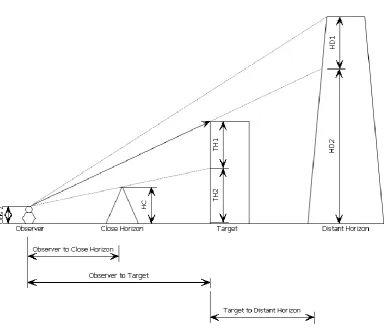
The „Close Horizon‟ is calculated by locating the feature directly in front of the target which creates the steepest viewing angle between observer and target, not including the FOI itself. The elevation of this object, known from the DSM, is used to calculate the intercept of a line of sight with the target, and deduce how much of the target is visible (Figure 2.5 - TH1). The obscured area is also recorded (Figure 2.5 - TH2).

2.5.2.2 Distant Horizon

By extending the LOS ray beyond the target it is possible to discover if the target makes the skyline, or is overshadowed by a more distant object. The search continues until either it intercepts the DSM, or reaches the same elevation as the maximum elevation in the DSM dataset. If the ray intercepts the DSM then the „Distant Horizon‟ location is recorded along with the elevation value at that point, and both distance behind target and extent of the object showing

(Figure 2.5 - HD1) are calculated. If no feature is found the target is designated as being on the skyline.

Figure 2.5: Line of Sight Details; the Close Horizon is used to calculate how much of the target is visible; the Distant Horizon information indicates whether the target is on the skyline

(30)

23 The values stored from each of the LOS calculations between the observer and each target point are summarised in Table 2-1.

Table 2-1: Line of Sight Target Return Values

Criteria Data Type Details

Visible Boolean

(True or False)

Whether a target point can be seen or not from current location

Target Location Point (x,y) The location of the target point

Target Elevation (TH1+TH2)

Metres (vertically) The height of the target point

Distance from Observer (Distance O-T)

Metres (horizontally) The distance from observer to target point

Close Horizon Location

Point (x,y) The location of the tallest object in the line of sight from the observer to the target

Close Horizon Height (HC)

Metres (vertically) The height of the tallest object between observer and target

Close Horizon Intercept With Target (TH1)

Metres (vertically) The amount of target which shows above the tallest near object

On Skyline Boolean

(True or False)

Whether the target has a taller visible object behind it, or sky

Distant Horizon Location

Point (x,y) The location of the intercept with a taller object behind the target (if any)

Distant Horizon Distance Behind Target (Distance T-DH)

Metres (horizontally) The distance from the target to the horizon

Distant Horizon Elevation (HD1+HD2)

Metres (vertically) The elevation of the item on the horizon visible behind the target

Distant Horizon Intercept (HD1)

Metres (vertically) The amount of the horizon that is visible above the target

Elevation Showing as Ratio Of Distance to Observer Ratio (TH1 /Distance O-T)

Ratio Considering any near horizons, calculate the ratio of visible vertical extent divided by distance to observer

2.5.3 Visibility at Feature Level

(31)

[image:31.595.114.479.125.472.2]

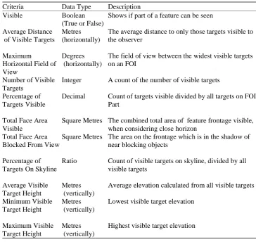
24 Table 2-2: Visibility Metrics at FOI Part level

Criteria Data Type Description

Visible Boolean

(True or False)

Shows if part of a feature can be seen

Average Distance of Visible Targets

Metres (horizontally)

The average distance to only those targets visible to the observer

Maximum

Horizontal Field of View

Degrees (horizontally)

The field of view between the widest visible targets on an FOI

Number of Visible Targets

Integer A count of the number of visible targets

Percentage of Targets Visible

Decimal Count of targets visible divided by all targets on FOI Part

Total Face Area Visible

Square Metres The combined total area of feature frontage visible, when considering close horizon

Total Face Area Blocked From View

Square Metres The area on the frontage which is in the shadow of near blocking objects

Percentage of Targets On Skyline

Ratio Count of visible targets on skyline, divided by all visible targets

Average Visible Target Height

Metres (vertically)

Average elevation calculated from all visible targets

Minimum Visible Target Height

Metres (vertically)

Lowest visible target elevation

Maximum Visible Target Height

Metres (vertically)

Highest visible target elevation

2.5.3.1 Field of View

Most of these metrics are self-explanatory, however „Field of View‟ and „Total Face Area‟ require clarification. The „Field of View‟ is calculated between the most extreme targets visible, which make the widest angle. If an object obscures a side of the FOI frontage then the FOV angle will decrease. However if an object blocks a portion in the middle of the FOI with the outside targets still visible, the FOV will return the widest viewing angle calculated from the outside points, ignoring the obscured portion of the FOI frontage.

2.5.3.2 Total Face Area – Visible / Blocked

(32)

25

Figure 2.6. Total Face Area Visible for a Feature of Interest

A number of derived metrics may also be useful such as the ratio of distant horizon height showing (HD1) over distance behind target, to give an indication of dominance of any distant features. Also the total visible face area divided by the average distance to the targets would give an indication of the presence of an FOI from the user‟s viewpoint.

2.6 Implementation and Evaluation

(33)

[image:33.595.151.456.72.576.2]

26

(34)

[image:34.595.86.501.182.474.2]

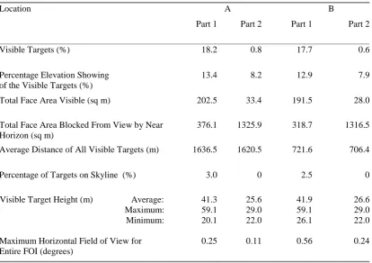
27 Table 2-3 shows the results from running the visibility calculations. The third part of the FOI was not visible from either location A or B, and has been removed from the table.

Table 2-3 Results from Sites A and B

Location A B

Part 1 Part 2 Part 1 Part 2

Visible Targets (%) 18.2 0.8 17.7 0.6

Percentage Elevation Showing of the Visible Targets (%)

13.4 8.2 12.9 7.9

Total Face Area Visible (sq m) 202.5 33.4 191.5 28.0

Total Face Area Blocked From View by Near Horizon (sq m)

376.1 1325.9 318.7 1316.5

Average Distance of All Visible Targets (m) 1636.5 1620.5 721.6 706.4

Percentage of Targets on Skyline (%) 3.0 0 2.5 0

Visible Target Height (m) Average: Maximum: Minimum: 41.3 59.1 20.1 25.6 29.0 22.0 41.9 59.1 26.1 26.6 29.0 22.0

Maximum Horizontal Field of View for Entire FOI (degrees)

0.25 0.11 0.56 0.24

The majority of the results are as expected with the more distant site showing the FOI to occupy a narrower field of view, that the spire (FOI Part 1) is visible, and none of main building (FOI Part 2) makes the skyline due to the tall surrounding buildings.

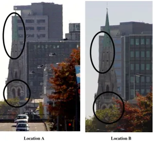
However the results show that the percentage elevation of visible targets (13.4% at A, 12.9% at B), percentage of targets on the skyline (3% at A, 2.5% at B), and total face area visible (202m2 at A, 191m2 at B) for the spire (FOI Part 1) go against the expected trend and are slightly greater at Location A than B. It is also noticeable that a greater extent of the spire is visible at location A (20.1m to 59.1m at A, and 26.1m to 59.1m at B).

(35)

28

[image:35.595.144.460.93.384.2]

Location A Location B

Figure 2.8. Comparison of Cathedral Spire from Locations A and B

2.6.1 Additional Analysis

Five further test locations (Figure 2.9) were selected and the metric results calculated. Values for total visible area frontage along a transect line passing from Location C, through D, and E are shown in Figure 2.10.

A statue and several trees block the view of the Cathedral along this approach, as reflected by the metrics.

(36)

29

Figure 2.9. Cathedral Square Test Sites (LiDAR data sourced from Christchurch City Council)

The main difference in the view between locations F and G is the proximity of a Police hut (Figure 2.11). At Location F, the Café (FOI Part 3) is not visible, whilst at Location G it scores 6.5% (percentage elevation of visible targets).

(37)

30 The total face area of the spire at Location F is 615.1m2, whilst at Location G it receives a value of 818.3m2. These are in agreement with the photographic evidence.

[image:37.595.156.404.363.741.2]

Location F Location G

Figure 2.11. Site F and G photographs

There is an interesting relationship between the field of view, and total area visible. Figure 2.12 illustrates this by considering 26,753 locations around Cathedral Square spaced 1 metre apart.

(38)

31 Close to a feature the field of view metric scores high, and the total frontage face area visible is low. As can be seen from the graph the points which contribute to the peak of face area value points (Set 1) are located away from the Cathedral on the edge of the square, whilst the highest FOV values (Set 2) are near the Cathedral. From a viewing experience the face area values may be considered the most appropriate metric to reflect „how much‟ of an FOI can be seen, and should be considered with distance to quantify the presence of an FOI.

2.6.2 Mapping the Visibility Metrics

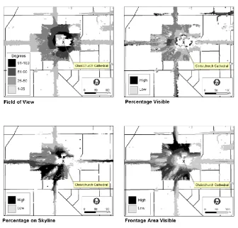
[image:38.595.132.469.314.635.2]

The values from the LOS implementation may be mapped to indicate how a user‟s experience of an FOI would vary across space (Figure 2.13). In this example the area in front of the Cathedral between test locations C and D (Figure 2.9) enjoys the highest visible percentage of targets, essentially the clearest view.

Figure 2.13. Maps of Key Metrics

(39)

32

2.6.3 Using the Visibility Metrics

These metrics combined with other GIS datasets can provide an LBS with the ability to be context-aware when delivering information to a user. When searching spatial databases the visibility metrics may be used to rank the results showing the most visible items first. In way-finding, the visible area values may be used to lead the user towards good viewpoints for nominated landmarks. Any information delivered to the user would need to be supported by additional datasets, such that attributes including the FOI‟s name, address, usage, and history could be conveyed to the pedestrian.

Although not implemented at this stage, a fuzzy logic layer will be introduced in the next phase of the research so that a natural language engine may select the most appropriate English terminology to describe the scene. This will allow the LBS to take on the role of a virtual city guide. The class limits will be set after conducting user trials to evaluate perceived object visibility against the metric results.

To ensure the LBS remains responsive to the user‟s movements, the metrics must be available in real time. This can be achieved in a number of ways. One method is to pre-cache the results for an area of interest, such that the mobile client requires only a simple lookup of the corresponding FOI visibility summaries.

An alternative approach, which will be used for the next phase of this research, is to implement a client-server architecture whereby a mobile client sends the user‟s location information across a network to the server which returns the visibility results for the surrounding region. Pre-caching on the server side is also possible such that the most commonly visited areas can be held in memory for improved response times.

2.7 Conclusion and Future Work

This research has shown that a line of sight algorithm may be used to supply a number of useful contextual visibility metrics from a LiDAR dataset in an urban environment. These results form part of a function of visibility which can be used to prioritise information on features of interest from the current observation location.

We have shown that it is possible to incorporate a wide range of visual statistics into reports of object visibility, with consideration of the surrounding cityscape, and the importance of close and distant horizons.

There are a number of areas for further research in this field. The algorithm considers only the physical aspects of visibility which can be calculated from a DSM. It currently neglects to consider the time of day, or weather in the visibility calculations.

(40)

33 indicate how easily an FOI may be resolved from its background. Aerial imagery might offer a partial solution suitable for identifying vegetation backgrounds, but roof top colours will not assist in contrast and colour information from the user‟s viewpoint, so georeferenced street level photography would be preferable.

Partial visibility through vegetation (Llobera 2007a) could be explored such that lines of sight are able to pass through, and under, canopy layers. The algorithm should be extended to accommodate seasonal tree canopy and vegetation density variation. It would also be worthwhile to examine raw LiDAR returns to produce detailed surfaces for the canopy layer.

Currently a scan in the vertical axis over the FOI returns information on the distant horizon. This could also be applied across the horizontal axis so that the surroundings may be used as context to determine if an FOI profile is significantly different from its neighbours (e.g. skyscraper amongst low rise buildings).

Referencing a number of FOIs in the metrics would allow a LBS to use relative descriptions of space, such as “the Chalice monument is visible to the right of the Cathedral”. Accessing models from the Google 3D Warehouse may also be useful such that pictorially the shape and texture of FOIs could be displayed, allowing the user to more easily identify the target FOI from surrounding buildings.

The ultimate goal of this research would be a single visibility function which considers weighted metrics based on visibility, architectural interest, building form, and social factors such as building use or related interests to the user, that would allow an LBS to rank in order from a scene those items which a viewer would consider most interesting. The values would then be passed through a fuzzy logic layer and a natural language engine to generate appropriate sentences to convey to the user descriptions of their surroundings, such that the LBS acts as a virtual city guide.

2.8 Acknowledgements

(41)

34

Chapter 3:

Advancing Visibility Modelling Algorithms for

Urban Environments

3.1 Summary

This chapter presents a number of methods for calculating the visibility of landmark features in the urban context. While current visibility modelling techniques establish which regions may be viewed from a location, it is sometimes necessary to quantify how much of a designated feature is visible from its surroundings. This is particularly relevant in the field of Location Based Services, where information is currently filtered using proximity and syntax matching, but could include more advanced egocentric and contextual filtering capabilities if feature visibility modelling was available. This research presents a method to establish the visible extents of landmarks in an urban environment, through the development of a number of visual metrics. These metrics are tested in both synthetic and real world trials.

3.2 Introduction

Standing in Trafalgar Square (London) it is possible to see Nelson‟s column, The National Gallery, and many statues and fountains. The space is largely defined by the visual field; which icons can be seen, their relative locations and how clearly they are in view. These landmarks are prominent features because of their visual, semantic or architectural attraction (Raubal and Winter 2002), and form useful reference points (Millonig and Schechtner 2007) which assist in building a mental model of the region useful for navigation and exploration (Fisher-Gewirtzman and Wagner 2003). Currently Location Based Services (LBS) under-use landmark visibility modelling (May et al. 2005), and rely on more simplistic proximity filters. However by introducing visibility modelling a LBS would be able to more closely match the user‟s experience and determine the impact of landmarks within the visual field. This chapter presents a novel method for quantifying landmark visibility with the eventual aim of providing the foundation for natural interaction with the user that aligns with their mental models, and matches their visual experiences.

Advances in Visibility Modelling in Urban Environments to Support Location Based Services