DOI: 10.1002/qj.3319
R E S E A R C H A R T I C L E
The moist parcel-in-cell method for modelling moist convection
David G. Dritschel
1Steven J. Böing
2Douglas J. Parker
2Alan M. Blyth
2,31Mathematical Institute, University of St Andrews, UK
2School of Earth and Environment, University of Leeds, UK
3National Centre for Atmospheric Science, University of Leeds, UK
Correspondence
David G. Dritschel, Mathematical Institute, University of St Andrews, St Andrews KY16 9SS, UK.
E-mail: david.dritschel@st-andrews.ac.uk
We describe a promising alternative approach to modelling moist convection and cloud development in the atmosphere. Rather than using a conventional grid-based approach, we use Lagrangian “parcels” to represent key dynamical and thermody-namical variables. In the prototype model considered, parcels carry vorticity, mass, specific humidity, and liquid-water potential temperature. In this first study, we ignore precipitation, and many of these parcel “attributes” remain unchanged (i.e. are materially conserved). While the vorticity does change following the parcel motion, the vorticity tendency is readily computed and, crucially, unwanted numerical diffu-sion can be avoided. The model, called “Moist Parcel-In-Cell” (MPIC), is a hybrid approach which uses both parcels and a fixed underlying grid for efficiency: advec-tion (here moving parcels) is Lagrangian whereas inversion (determining the velocity field) is Eulerian. The parcel-based representation of key variables has several advan-tages: (a) it allows anexplicitsubgrid representation; (b) it provides a velocity field which isundampedby numerical diffusion all the way down to the grid scale; (c) it does away with the need for eddy viscosity parametrizations and, in their place, it provides for a natural subgrid parcel mixing; (d) it isexactly conservative(i.e. there can be no net loss or gain of any theoretically conserved attribute); and (e) it dis-penses with the need to have separate equations for each conserved parcel attribute; attributes are simply labels carried by each parcel. Moreover, the latter advantage increases as more attributes are added, such as the distributions of microphysical properties, chemical composition and aerosol loading.
K E Y W O R D S
convection, clouds, numerical method
1 I N T R O D U C T I O N
Clouds, convection and moist processes generally pose seri-ous challenges for modelling the Earth’s climate and weather (e.g. Hollowayet al., 2014; Bonyet al., 2015). Such processes involve small-scale interactions which are well beyond the resolution of current global circulation models (GCMs). In particular, accurate resolution of processes influenced or con-trolled by turbulence in clouds requires model scales of the order of metres (Austinet al., 1985; Blythet al., 2005; Cooper
et al., 2013; Heinzeet al., 2015; Seifertet al., 2015), scales
which are more than seven orders of magnitude smaller than the global scale!
The large-eddy simulation (LES) method has been used to study cumulus and stratocumulus clouds since the pio-neering work of Sommeria (1976) and Deardorff (1980). In LES, the impact of subgrid-scale motions on resolved scales is modelled by turbulence closure assumptions. LES models play a key role in the development of low cloud parametrizations (e.g. Siebesma and Cuijpers, 1995) and have been routinely validated for observational cases (e.g. Brown
et al., 2002; Siebesmaet al., 2003). Other non-hydrostatic
This is an open access article under the terms of the Creative Commons Attribution License, which permits use, distribution and reproduction in any medium, provided the original work is properly cited.
© 2018 The Authors.Quarterly Journal of the Royal Meteorological Societypublished by John Wiley & Sons Ltd on behalf of the Royal Meteorological Society.
models have also been essential in studying the interaction between deep convection and its environment (e.g. Bretherton and Smolarkiewicz, 1989), and mixing at the edge of clouds (Grabowski and Clark, 1993). However, there are key differ-ences between two-dimensional and three-dimensional simu-lations of deep convection (Redelspergeret al., 2000; Petchet al., 2008), and three-dimensional LES on large domains has only become possible over the last decade (Khairoutdinovet al., 2009). Detailed cloud models have also been used both as embedded models for local weather forecasting (Schalkwijket al., 2015) or as subgrid models in larger-scale models (“super-parametrization,” e.g. Grabowski and Smolarkiewicz, 1999). The need for a high-resolution description of cloud turbu-lence is due to the highly nonlinear nature of cloud processes. Previous studies have shown that the behaviour of cumulus clouds is very sensitive to the choice of numerical method (Matheou, 2011; Presselet al., 2015). The equations of state describing the transfer between different phases of water involve very steep functions, usually represented by discon-tinuous changes. Furthermore, aircraft measurements have shown that the thermodynamic properties of clouds can have large variations on scales of metres to tens of metres (Austinet al., 1985; Blythet al., 2005), and cumulus clouds often contain cores with relatively high liquid water content (Heymsfield et al., 1978; Blythet al., 2005; 2015; Moser and Lasher-Trapp, 2017). Such regions may be important in determining the time-scale for rain formation (Twomey, 1966; Blyth et al., 2013; Cooper et al., 2013). Resolving these scales of motion appears to be essential to modelling cumulus convection.
The computational demands for high-resolution cloud sim-ulation are exacerbated when consideration is made of addi-tional attributes of the air parcels, such as the distributions of microphysical properties (e.g. drop sizes), chemical com-position and aerosol loading. Accurate treatment of cloud microphysics demands consideration of droplet size distribu-tions of cloud water and cloud ice distribudistribu-tions: the ice is itself divided into many possible classes (according to crys-tal form, aggregation, etc). For instance, a model may carry
N ∼ 6 species of water and ice withM ∼ 50 bins. Clouds are also important agents of transport and chemical trans-formation of trace gases in the climate system, and many of the chemical reactions are nonlinear and occur on the fine scales within a cloud. Sophisticated cloud-chemistry schemes may include many interacting species. Aerosols feed back on the cloud physics by acting as condensation nuclei and modifying the distributions of cloud particles. For these rea-sons, a sophisticated cloud-resolving model capable of study-ing cloud–chemistry–climate processes may need to carry cloud microphysical spectra, aerosol spectra and a number of interacting chemical species on its grids. These addi-tional attributes place enormous demands on computaaddi-tional resources – involvingboththe cost of dynamical transportand
that of additional processes such as chemical reactions – and
are included at the expense of the resolution needed to capture cloud fine structure.
There is hence a pressing need to improve the numerical modelling and representation of moist processes in general. Previous studies have considered whether methods used in the computer graphics and gaming community can help to pro-vide simulations with a higher effective resolution at reduced computational cost (e.g. Shutts and Allen, 2007). In this paper, we also propose a non-standard approach, namely to represent dynamical and thermodynamic processes by freely movingparcels. The parcels carry a number of attributes, such as vorticity, mass, specific humidity, and liquid-water potential temperature. Ignoring precipitation, the attributes of mass, specific humidity and liquid-water potential temper-ature are all conserved following the motion of each parcel, and importantly a parcel-based model guarantees this with-outthe need to follow additional prognostic equations as in a conventional numerical model. The advantages grow when more attributes are considered, such as a spectrum of aerosol particle sizes, chemical species, etc. Moreover, the parcels provide an explicit sub-grid parametrization – indeed they replace the need for such a parametrization – thereby dis-pensing withad hoc parametrizations and artificial “eddy” viscosities. Mixing on the smallest scales can be dealt with by parcels splitting and recombining.A priori, a parcel-based model has much less numerical dissipation than conventional numerical models presently in widespread use. Hence, a parcel-based model can be expected to achieve a much higher effective resolution.
Parcel-based methods are not new: they have been used in the vortex dynamics literature for decades to study basic properties of fluid flows at very high Reynolds numbers (e.g. Christiansen and Zabusky, 1973 for two-dimensional flows, and Novikov, 1983, Aksman et al., 1985,
Ander-son and Greengard, 1985, Alkemade et al., 1993 for
three-dimensional flows). Such methods have even been used to model moist convection as early as Gadian (1991), who simulated clouds in a two-dimensional plane using Smoothed Particle Hydrodynamics (SPH). This method in fact originated in studies of astrophysical phenomena (Mon-aghan, 1992), and continues to be a popular choice in mod-elling galaxy dynamics, star formation and stellar clusters (e.g. Smilgys and Bonnell, 2017). In atmospheric chem-istry and transport studies, parcel-based methods such as the Finite Mass Method (FMM; Klinger et al., 2005 and ref-erences therein) and the Hamiltonian Particle-Mesh method (HPM; Frank et al., 2002) have been shown to offer sig-nificant improvements over the commonly used grid-based
semi-Lagrangian method (Grewe et al., 2014). The HPM
a dynamical core that is otherwise Eulerian (e.g. Andrejczuk
et al., 2008; Shima et al., 2009; Riechelmann et al., 2012; Wyszogrodzkiet al., 2013). Nevertheless, to our knowledge, a parcel-based method has never been seriously considered to be a viable approach for detailed cloud modelling.
Parcel and particle-based methods vary considerably in their formulation, and may require the tuning of many numer-ical parameters. We believe that this has detracted from the uptake of such methods by the atmospheric modelling com-munity. Here, in order to produce a flexible, versatile model with a minimum of tunable parameters, we adopt the simplest “vortex-in-cell” (VIC) approach of Christiansen and Zabusky (1973), with a parameter-free refinement due to Brackbill and Ruppel (1986) to ensure conservation. We also use the math-ematically reformulated parcel vorticity equation of Cottet and Koumoutsakos (2000, pp. 244–245) to more accurately satisfy the non-divergence condition of the vorticity field. Moist processes, specifically the effects of condensation and evaporation, are incorporated in a simplified way and in an idealized physical setting, with the sole purpose of providing a proof of concept.
The resulting new model, called “Moist Parcel-In-Cell” (MPIC), is extensively tested to understand dependencies on numerical parameters and to determine feasible values. As a demanding test case, we consider the evolution of a rising moist thermal in a neutral layer below a stratified zone. The thermal reaches the stratified zone and passes through the lifting condensation level where it releases additional buoy-ancy and forms a cloud. The flow evolution rapidly becomes turbulent, and is reminiscent of observed cumulus convec-tion. Comparisons with a convection-permitting research model, the Met-Office/NERC cloud model (MONC) are the focus of a forthcoming paper (Böing et al., forthcoming). There, and in one figure here, the MPIC model is shown to compare well using significantly lower grid resolutions. This is the result of using a conservative sub-grid representation in the MPIC model, thereby greatly reducing the effects of numerical diffusion.
The plan of the paper is as follows. Section 2 describes the idealized physical setting considered, and sets out the associated simplified mathematical model. Section 3 then details the MPIC numerical method, focussing in particular on its novel or non-standard features. Section 4 goes through a series of tests which demonstrate the insensitivity of the results to the only tunable parameters, those controlling par-cel density and mixing. Finally, section 5 concludes with a discussion of the steps currently being taken to extend the MPIC model to more realistic physical settings.
2 P H Y S I C A L S E T T I N G A N D M A T H E M A T I C A L F R A M E W O R K
Cloud formation in the atmosphere is a highly com-plex process. We do not attempt to model every aspect
of this process, but only intend to demonstrate a viable computational approach that could lead to a step change in modelling atmospheric convection in general. To this end, we consider a simplified physical setting in an idealized geom-etry, and reduce the governing mathematical equations to their simplest relevant form. Key aspects of the dynamics and physics are retained, notably the inclusion of a latent heating term with a nonlinearity characteristic of more sophisticated cloud schemes.
First, we assume the domain is Cartesian, horizontally
peri-odic in x (0 ≤ x ≤ Lx) and in y (0 ≤ y ≤ Ly), and
bounded below and above by flat, impermeable, free-slip
surfaces at z = 0 and Lz. Second, we make the
incom-pressible Boussinesq approximation (Durran and Arakawa, 2007) in which variations in density are small compared with the domain average density. This is not valid for deep con-vection, but is often used in studies of shallow convection (Brown et al., 2002; Siebesma et al., 2003). This approxi-mation greatly simplifies the governing equations, but it is not required by the MPIC model (section 5 below). Third, we simplify the pressure–temperature dependent formula-tion of saturaformula-tion specific humidity occurring when moisture within an air parcel condenses or evaporates. Instead, the effects of latent heating are included by increasing the parcel buoyancybwhenever the parcel specific humidityqexceeds a height-dependent background profileq0e−𝜆z (with𝜆
con-stant). Effectively, the saturation specific humidity depends only on height. Thus, a moist parcel can gain buoyancy (tend-ing to accelerate upwards) when its water vapour condenses. Likewise, it can lose buoyancy when it evaporates. Conden-sational heating is the only effect of moisture that we account for: we ignore differences in density between dry air and water vapour, as well as the weight/loading of condensate.
The simplicity of this framework has been designed so that the first development of the model, and the analysis of its performance, focusses on the essentially Lagrangian dynamical core. In particular, we have constructed a model framework which is simple enough to isolate the dynamical behaviour without additional complicating processes, such as microphysical feedbacks. In this framework, we are able to characterize the dynamical performance quantitatively and definitively. The simple framework will make it easy for oth-ers to replicate our results, and it also ensures the equations lend themselves to non-dimensionalization. The key feature of the thermodynamics that we have retained is the disconti-nuity in the equation of state that is a result of condensation. There are some precedents for making the saturation specific humidity depend on height only: for example, Pierrehumbert
et al.(2007) and Tsang and Vanneste (2017) essentially use the same formulation. However, in their case, liquid water is assumed to be removed (precipitate), whereas in our case liquid water does not precipitate but can re-evaporate.
domain heights, as the liquid water content here depends on height as well as two other thermodynamic variables. How-ever, the interpretation of the thermodynamic variables in this framework is less straightforward. Moreover, once a parcel is saturated, the amount of condensation per unit height is con-stant rather than exponentially decreasing in this formulation, which makes it less appropriate for deeper domains.
Our ongoing work in the development of the model will add increasing degrees of sophistication to the microphysical representations. It would be relatively simple to replace our thermodynamic formulation with a saturation specific humid-ity which depends on temperature and a height-dependent reference pressure. In this case, we would need to include an iterative procedure for solving the equation of state. Usually, some simplifications are made in the thermodynamics, and different models use a variety of formulations. The details do not matter for a proof of concept, and this is why we have taken the simplest approach.
The governing equations written in momentum form for velocity u, (non-hydrostatic) pressure p, liquid-water buoy-ancybland specific humidityqare
Du
Dt = −
𝜵p 𝜌0
+b̂ez, (1)
Dbl
Dt =0, (2)
Dq
Dt =0, (3)
𝜵⋅u=0, (4)
where D∕Dt = 𝜕∕𝜕t +u⋅ 𝜵 is the material derivative. In Equation 1 the total buoyancyb(including the effects of latent heating) is approximated by
b=bl+
gL cp𝜃l0
qc, (5)
where
qc=max
(
0,q−q0e−𝜆z) (6)
is the liquid water content. The pressure p in Equation 1 excludes the part due to the hydrostatic background state of constant density 𝜌0. The other symbols appearing in
Equations 1–6 are the vertical unit vector ̂ez, the gravita-tional acceleration g, the latent heat of condensationL, the specific heat at constant pressure cp, the surface saturation humidity q0, and the inverse condensation scale-height 𝜆. The liquid-water buoyancy is defined bybl=g(𝜃l−𝜃l0)∕𝜃l0
where𝜃lis the liquid-water potential temperature and𝜃l0is a
constant reference value.
The incompressible Boussinesq approximation is conve-nient since, in the vorticity formulation, the pressure term disappears. The vorticity𝝎=𝜵×usatisfies
D𝝎
Dt =𝝎⋅𝜵u+
(
by,−bx,0
)
, (7)
where subscripts on bdenote partial differentiation. Hence, vorticity is generated by horizontal buoyancy gradients.
Notably, regions of the flow with uniformband no vorticity remain irrotational (𝝎=0).
Small-scale models of deep convection usually employ an anelastic formulation of the continuity equation (Pauluis, 2008) rather than the incompressible Boussinesq approx-imation we are using here. In the near future, we aim to extend MPIC to the anelastic framework by weighting both its conserved properties and the parcel volumes by a height-dependent mean density𝜌0(z), and by making
appro-priate changes to the numerical solver. To use MPIC as an embedded model, it would also be important to ensure max-imum consistency in the thermodynamical formulation with the host model (Grabowski and Smolarkiewicz, 2002).
Finally, we ignore precipitation. However, the Lagrangian method for precipitation introduced by Shimaet al. (2009) would be one of the ways in which this could be added. We plan to include precipitation in a future version of MPIC.
3 T H E N U M E R I C A L A L G O R I T H M
We first present an overview of the algorithm, then describe how it is constructed and provide details of features not found in other parcel-based numerical methods.
Lagrangian, freely-moving parcels are used for evolving all quantities, while an underlying regular (here Cartesian) grid is used for transferring parcel properties to the grid and vice versa. The grid is also used for “inversion,” i.e. to obtain the velocity field from the interpolated vorticity field. This is the basis for the original Vortex-In-Cell (VIC) method (see Christiansen and Zabusky, 1973 and the com-prehensive review of Cottet and Koumoutsakos, 2000). The parcels are ideal for carrying quantities which do not change in time – materially conserved quantities called “attributes.” In the present model, the attributes consist of liquid-water buoyancybl, specific humidity qand parcel volumeV. No additional equations are required to evolve the attributes as in a grid-based model; the attributes are merely labels carried by each parcel. Instead, the positionsxiof each parceliare evolved using the simple equation
dxi
dt =u(xi,t), (8)
But what is most remarkable is that this remaining part contributes nothing to the velocity field (though it is needed in the vorticity tendency equation).
A potential drawback of parcel-based methods is that large numbers of parcels must be superposed to accurately rep-resent any evolving flow. In the original applications to a uniform density fluid, parcels could be restricted to a small volume of the entire space, as in that case no new vortic-ity is produced outside of its initial domain of support. In a variable-density flow, vorticity does not remain localized if initially so. Hence, in the MPIC model, we fill theentire
domain with parcels, ensuring each grid box contains many parcels (typically 5–200). We originally thought this would be computationally prohibitive, but it turns out to be affordable, especially when compared to conventional numerical models. Essentially, we have found that the higher effective resolution afforded by the parcels – and the strict conservation of par-cel attributes – strongly offsets the costs of carrying a large number of space-filling parcels. The operations performed on parcels are mostly simple interpolations (see below) which are relatively inexpensive from a computational point of view.
Another well-known problem with parcel methods is that the parcel motion does not respect exact mass conservation or incompressibility (Greweet al., 2014). While each parcel carries a volume, and the parcel advection is accurate, using a finite number of parcels inevitably leads to numerical density anomalies, even if care is taken initially to ensure a perfect match between the parcel and grid densities (or volumes in an incompressible flow). This problem can be alleviated by con-servatively adjusting parcel properties (e.g. as in Greweet al., 2014), but its seriousness depends on the number of parcels used to find a given field on the grid, and the duration of the flow simulation. Grabowskiet al.(2018) describe a scheme in which the interpolated velocity field is incompressible throughout each grid box, but even this does not guarantee that the parcel density remains uniform (as the example of a single parcel crossing a grid box boundary demonstrates). In the results presented below using the MPIC model, we find that the discrepancy between parcel and grid densities is neg-ligible over cloud development time-scales when using the recommended default numerical settings.
Parcels simplify many features of the dynamics. In partic-ular, the effects of condensation and evaporation on parcel buoyancy are naturally incorporated in a parcel formulation. All that is required is to construct the total buoyancybfrom the liquid-water buoyancybl, specific humidityqand parcel heightzusing Equation 5, then interpolatebto gridded values for calculating the parcel vorticity tendencies (section 3.1).
The MPIC model uses perhaps the simplest of all interpo-lations – tri-linear interpolation – to transfer parcel properties to and from an underlying grid. This interpolation is needed in order to build the vorticity field on a grid and to use effi-cient, accurate grid-based methods for calculating the velocity field from the vorticity field. The gridded velocity field is then
interpolated at the parcel positions, enabling one to move the parcels forward to the next instant of time. Other forms of interpolation (e.g. involving a search over nearby parcels as in SPH or HPM) may be more accurate, but are not nearly as simple, and may not lend themselves to efficient calculation on massively parallel computers. Notably, the interpolation used ensures that the total parcel mass, and indeed all par-cel attributes, are not only conserved but are identical to the grid-based calculation of the same quantities after interpola-tion (Brackbill and Ruppel, 1986; Cottet and Koumoutsakos, 2000, pp. 241–242).
In order to follow the inevitable, and often rapid, cascade of scales in a turbulent flow, we allow for parcel splitting down to a prescribed minimum scale. To decide when parcels should split, we keep track of each parcel’s “stretch”: the time inte-gral of the magnitude of the vortex stretching. (Note: a more robust measure of parcel stretch would make use of the local strain tensor𝜵u, but this requires tracking the parcel shape (five extra variables) as in McKiver and Dritschel, 2003.) When the stretch exceeds a certain threshold (around four in practice, though the results are insensitive to this, as shown in section 4), we split the parcel into two adjacent pieces, each with half the volume of the original parcel but with identical attributes and vorticity. This splitting is designed to be fully conservative: the total volume-integrated parcel attributes do not change.
However, splitting cannot be allowed to carry on indefi-nitely, as it would lead to an explosive build-up in the total number of parcels. Hence, we limit the volume of the smallest parcel to 1∕63or 1∕216 of the grid-box volume, and remove
smaller parcels conservatively (section 3.5 below). Again, the accuracy of the model is not sensitive to this parameter as long as it is substantially smaller than the original parcel volume (as shown in section 4).
The principle behind this is that there is a trade-off between representing subgrid-scale effects and ignoring subgrid-scale velocity fluctuations (in the interpolation of parcel velocities from gridded values). Parcel motions are generally dominated by the larger-scale velocity field, but this cannot be expected to hold for too great a separation between the parcel size and the grid size. Nonetheless, a subgrid representation may be highly beneficial, as has been demonstrated in contour-based, Lagrangian simulations of two-dimensional fluid and mag-netized turbulence (Dritschel and Ambaum, 1997; Dritschel and Scott, 2009; Fontane and Dritschel, 2009; Dritschel and Fontane, 2010; Dritschel and Tobias, 2012).
In two dimensions, velocity fluctuations tend to decay more rapidly with decreasing scale than in three dimensions. The kinetic energy spectral density(k)in two dimensions often exhibits ak−3 form for large wavenumberk, while in three
dimensions (k) ∼ k−5∕3 (Davidson, 2015). As (k) ∝ k‖̂u‖2, this means that velocity fluctuations ‖̂u‖ typically
decay like k−2 in two dimensions and like k−4∕3 in three
velocity field, but the small scales are much more active in three dimensions.
Previous studies of two-dimensional turbulence conducted using contour-based Lagrangian methods have shown that the scale separation between the finest resolved Lagrangian element and the grid scale can be as large as a factor of 16, while still faithfully representing the flow field (in particular, Dritschel and Scott, 2009 and Dritschel and Tobias, 2012). In the present context, in three dimensions, we do not expect such a large scale separation, and our choice of a factor of 6 is explained and justified in the results below.
As in parcel splitting, we ensure parcel removal is exactly conservative. Each parcel transfers its vorticity and attributes to the corners of the grid box containing it before it is removed. These residuals are then re-interpolated to the remaining parcels to ensure conservation. Notably, this acts as a weak diffusion: a localized parcel disperses its properties to all other parcels in its grid boxas well asin the grid boxes adjacent to this grid box.
3.1 The parcel vorticity equation
The parcel vorticity 𝝎i is updated using a mathematically equivalent form of the vorticity equation 7 applied to each parcel:
d𝝎i
dt =S(xi,t), (9)
where
S(x,t)≡(𝜵⋅F,𝜵⋅G,𝜵⋅H) (10)
is the vorticity tendency, and
F=𝝎u+b̂ey, G=𝝎v−b̂ex, H=𝝎w. (11)
In Equation 11,̂ex and̂eyare unit vectors in the xandy directions respectively.
The vorticity tendencySis first found on the grid and then interpolated to the parcel positions. Since 𝜵⋅ 𝝎 = 0, this tendency is equivalent to that on the r.h.s. of Equation 7. This form of the tendency is used because it better preserves 𝜵⋅𝝎p=0 for the parcel-interpolated vorticity field𝝎p( Cottet and Koumoutsakos, 2000, pp. 244–245), as we have ourselves verified. However𝝎pdoes not generally satisfy the solenoidal condition (which should hold if𝝎p = 𝜵×u). This discrep-ancy can be removed by finding a scalar potential𝜒(x,t)for which𝝎≡𝝎p−𝜵𝜒is solenoidal. This implies𝛻2𝜒=𝜵⋅𝝎p. So, while𝝎pmay be localized on a parcel,𝝎is generally not. One may think of𝜵𝜒as the field that threads all the parcels together to ensure vortex lines never end in the fluid. Remark-ably,𝜵𝜒 does not contribute to the gridded velocity fieldu, as shown in section 3.3.
3.2 Parcel interpolation
We next briefly describe the (mostly) standard means of transferring parcel properties to the underlying grid, and the inverse operation of interpolating grid properties at a
parcel position. In this subsection, a subscript i denotes a parcel quantity while an overbar as inq̄ denotes a gridded field.
In the MPIC model, both of these operations use tri-linear interpolation, a simple method based on dividing a grid box into sub-volumes which are then used as weights in the interpolation. For example, the gridded value of the specific humidity,q̄(x̄,t), at each grid pointx̄ = (x̄, ̄y, ̄z)is computed from
̄
q(x̄,t) =V̄−1 ∑
i∈(x)̄
𝜙(xi−x̄)qiVi (12)
with V̄(x̄,t) = ∑ i∈(x)̄
𝜙(xi−x̄)Vi, (13)
where the tri-linear weights𝜙are given by
𝜙(xi−x̄) =
(
1−|xi−x̄| Δx
) (
1− |yi−ȳ| Δy
) (
1−|zi−z̄| Δz
)
(14)
and(x̄)is the set of all parcels within the eight grid boxes surroundingx̄. HereΔx,ΔyandΔzare the grid lengths in the three coordinate directions. This interpolation scheme pre-serves the global integral of qas well as its first moments (integrals ofxq,yqandzq). Moreover, compared to the origi-nal VIC interpolation scheme that usedV̄ = ΔV, whereΔV≡
ΔxΔyΔzis the grid box volume, this scheme has the advan-tage that the variance ofqis non-increasing (Brackbill and Ruppel, 1986; Cottet and Koumoutsakos, 2000, pp. 241–242). In practice, it is not necessary to find the set(x̄)directly; instead we sum over all parcelsiand work out the grid box they are contained within. From this, we add appropriately weighted parcel properties to the eight corner grid points.
After interpolation, the volumes V̄(x̄,t) of boundary grid points (atz = 0 andLz) are doubled since these grid points are surrounded by only four grid boxes rather than eight in the interior. Similarly, the sum in Equation 12 is either doubled or set to zero depending on symmetry of the field (section 3.3 below). The buoyancyb̄and specific humidityq̄
are set to fixed, uniform values at each boundary to simplify the inversion problem discussed in section 3.3, though this is not essential.
Note that, in an incompressible fluid, we would expect that
̄
V(x̄,t)remains constant and equal to the grid box volumeΔV
everywhere. However, Lagrangian parcel advection does not guarantee this. This may be regarded as a source of error, but in practiceV̄(x̄,t)differs little fromΔV if a sufficient num-ber of parcels are used, as the results in section 4 demonstrate. (With a minor change to the algorithm, we can enforce vol-ume conservation, but this comes at the expense of nvol-umerical diffusion; section 3.5 below.)
The reverse operation, to interpolate a gridded field value to a parcel positionxi(t), is performed as follows. For example, the velocity of a parcel is computed from
u(xi,t) =
∑
̄
x∈i
whereiis the set of all eight grid points at the corners of the grid box containing parceli.
3.3 The inversion problem
Since the domain considered is horizontally periodic, it makes sense to use Fourier series and Fast Fourier Transforms (FFTs) to perform operations on gridded fields. In the vertical, we also use Fourier series, for simplicity, though finite dif-ferencing would be more computationally efficient. Fourier series are not necessarily more accurate than second-order finite differences, particularly when fields exhibit shallow spectra, as is typical in turbulent flows (Shipton, 2008). Nonetheless, they allow for the most straightforward com-putational implementation. In fact, in the MPIC model,any
solver could be used which provides the velocity field and the vorticity tendency on a regular grid.
Here we discuss how we obtain the (gridded) velocity field
ufrom the vorticity field𝝎together with appropriate bound-ary conditions. This is a standard problem, but a few details are provided for clarity. In this subsection, the overbar on gridded quantities is dropped since there is no reference to parcel quantities.
For the incompressible flow considered, we can satisfy 𝜵⋅u=0 by takingu= −𝜵×AwhereAis a vector potential. From the definition of vorticity and basic vector calculus, we find
𝝎=𝜵×u=𝛻2A−𝜵(𝜵⋅A). (16) We are free to impose𝜵⋅A=0 leading to
𝝎=𝛻2A, (17)
a (vector) Poisson equation to determineA= (A,B,C)from 𝝎= (𝜉, 𝜂, 𝜁). To solve this, we must account for the boundary conditions atz = 0 andLz. First of all, the vertical velocity componentwmust vanish. The horizontal componentsuand
vmay be arbitrary (free slip). Asu=Bz−Cy, v=Cx−Az,
w=Ay−Bxand 𝜵⋅A=Ax+By+Cz=0, it is then sufficient to takeA=B=Cz=0 on each boundary.
Because we use Fourier series inz, we representAandBas a sine series, andCas a cosine series. It is most straightfor-ward to represent the vorticity components in the same way, which then implies𝜉 = 𝜂 =𝜁z = 0 on each boundary (note
𝜉 = −vzand𝜂=uzthere;uz =vz =0 is sometimes referred to as a “stress-free” boundary condition). This means vortex lines are perpendicular to each boundary and pass “through” them continuously. But for 𝜉 and 𝜂 to remain zero on the boundaries, it is necessary to take the buoyancybto be uni-form – then from Equation 7 there is no baroclinic vorticity generation.
Ifbis initially uniform on each boundary, in the absence of condensation there,bwill remain uniform (and constant) due to material conservation ofbl(Equation 2). In the future, we will allow arbitrarybvariations to study e.g. localized surface heating and moisture sources. Recoveringu from𝝎 in this
case is not as straightforward (cf. Cottet and Koumoutsakos, 2000, pp. 92–96).
In the numerical method, we use Fourier series inx,yandz
(with corresponding wavenumberskx,kyandkz). Depending on the field, either a sine series or a cosine series is used inz
to match the required boundary conditions. After an FFT, the Poisson problem Equation 17 reduces to an algebraic one, giving
̂
A= −𝝎̂∕|k|2 (18)
directly, wherek = (kx,ky,kz)and a hat indicates a spectral quantity. Note k=0 is excluded as the domain-averaged value of𝝎is zero. FromÂ, the velocity components in spec-tral space are found simply by wavenumber multiplication. Finally, an inverse FFT provides the velocity field u at all grid points.
The vorticity𝝎above includes the correction to the parcel vorticity𝝎pwhich makes it solenoidal, as discussed above in section 3.1. That is,𝝎≡𝝎p−𝜵𝜒 where𝛻2𝜒 = 𝜵⋅𝝎p. To solve this Poisson problem, we expand𝜒and the source𝜵⋅𝝎p in a Fourier sine series inzand obtain𝜒̂as in Equation 18. Notably this correction does not contribute to the velocity
usince𝜵×𝛻−2𝜵𝜒 =0 for the boundary conditions
consid-ered. Nonetheless it is included to more accurately compute the vorticity tendencySin Equations 10 and 11.
3.4 Filtering
A circular de-aliasing filter is applied to avoid spurious modes arising when computing the nonlinear product terms in the vorticity tendency Equation 10. The standard “2/3 rule” is applied, whereby we set to zero all coefficients with wavenumbers greater than 2/3 of the maximum wavenum-ber (Canutoet al., 2007). Rather than do this inkx,kyandkz separately, we instead apply the circular filter
F(k) =
{
1 k<2kmax∕3,
0 k≥2kmax∕3, (19)
where k = |k| and kmax =
√
(n2
x+n2y+n2z)∕6. This fil-ter is applied to the vorticity field𝝎when it is corrected to be solenoidal. The velocity fielduis then automatically fil-tered because of the linear relation between𝝎andu. No other filtering or damping is used.
3.5 Parcel splitting and mixing
In the MPIC model, the small-scale end of this cascade is modelled by parcel splitting and eventual removal at a pre-scribed smallest scale. While we do not follow the shape of each parcel, we do monitor the integrated vorticity stretching
𝛾i(t) =
∫
t
ti
(|𝝎i⋅d𝝎i∕dt|)1∕3dt, (20) whereti is the time when the parcel came into existence or last split. Then, when𝛾i(t)> 𝛾max, the parcel is split into two
adjacent pieces, each with half the volume of the original parcel but identical vorticity and attributes. Here, 𝛾max is a
non-dimensional numerical parameter which must be cho-sena priori. The default value is𝛾max = 4 but, as shown in
section 4, the results are not strongly sensitive to this choice. A smaller value causes splitting to occur more frequently, and
vice versa. An intermediate value represents a compromise between too frequent splitting and no splitting at all.
Note that parcel splitting, together with their eventual removal, helps to ensure that parcels do not stay undiluted for long times. In this way, some mixing of parcel properties occurs, as would be expected at sufficiently small scales in a turbulent flow.
When a parcel is split, it is replaced by two parcels sep-arated by a distance ds = (2Vi∕𝜋)1∕3 along the direction 𝝎i∕‖𝝎i‖of the original parcel’s vorticity vector. The formula fordscomes from imagining that the original “stretched” par-cel has the shape of a cylinder of radius Rand length 4R; this is then split into two adjacent cylinders separated by
ds = 2Rcentre to centre. More generally, it is consistent to takeds∕R∝𝛾max. However, the precise details do not matter;
up to 50% variations indshave no appreciable impact on the early to intermediate time flow evolution. If thezcoordinate of any new parcel lies belowz = 0 or aboveLz, it is placed back on the respective boundary.
A more robust model of stretching and splitting would allow each parcel to change shape, e.g. deform as an ellip-soid (McKiver and Dritschel, 2003), in response to the local strain tensor 𝜵u. While more physically based, this model would require tracking five additional variables, and has not been implemented for simplicity. Future work will examine its feasibility.
Over the course of a simulation, typically parcels continue to stretch and split, and thereby shrink in volume. When the volume Vi < Vmin, the parcel is mixed into the
surround-ings and removed from the list of parcels. Here, we use
Vmin = ΔV∕63 by default, but again the numerical results
are not strongly sensitive to this choice (section 4 below). The idea behind this parameter setting is to allow for some subgrid-scale representation, but to limit the scale separation of the smallest parcel and the advecting velocity field. The parcel motion is mainly controlled by velocity field varia-tions at larger scales, but this cannot be expected to hold for a wide scale separation. As discussed at the beginning of this section, a similar consideration applies in two-dimensional flows, where the scale separation can be much larger (up to a
factor of 16) owing to the greater regularity of the advecting velocity field (Dritschel and Ambaum, 1997; Fontane and Dritschel, 2009).
To maintain global conservation after mixing, the volumes
Vi and volume-integrated properties bl iVi,qiVi and𝝎iVi of all parcels to be removed are spread to the corners of the grid boxes they lie in, forming gridded residual fields. (In this subsection, we again use a subscriptito denote a parcel quantity and an overbar to denote a gridded field for clarity.) For example, at each grid point x̄ the residual volumeVres̄
and the residual volume-integrated specific humidityQres̄ are given by
̄
Vres(x̄,t) = ∑ i∈res(x)̄
𝜙(xi−x̄)Vi, (21)
̄
Qres(x̄,t) =
∑
i∈res(x)̄
𝜙(xi−x̄)qiVi, (22)
whereres(x̄)is the set of all parcels to be removed (if any) within the eight grid boxes surroundingx̄. (At the boundaries, where there are only four grid boxes above or belowx̄, both
̄
VresandQres̄ are doubled for consistency.)
Likewise we can define analogous quantities for the origi-nal parcels to be retained:
̄
Vori(x̄,t) = ∑ i∈(x)̄
𝜙(xi−x̄)Vi, (23)
̄
Qori(x̄,t) = ∑ i∈(x)̄
𝜙(xi−x̄)qiVi, (24)
where(x̄)is the set of all parcels to be retained within the eight grid boxes surroundingx̄ (with doubled values ofVorī
and Qorī at the boundaries). The sums of these quantities,
̄
Vori+V̄resandQ̄ori+Q̄res, respectively equalV̄ andQ̄ before
any parcels are removed.
The aim is to useV̄resandQ̄resto adjustViandqiso that
• the sums ofVi and of Qi over all parcels equate to the original sums before any parcels were removed, and
• the sums ofV̄ andQ̄ over all grid points also equate to the original, and same, sums.
This adjustment can in fact be done in many ways. Here, we adjust volumes and propertiesin proportion tothe orig-inal parcel volume Vi. This means that all parcels grow by the same fraction (for reasons mentioned below). To ensure global conservation, we must then divide Vres̄ and Qres̄ by
̄
Voribefore interpolating the residuals to the parcel positions.
As a result, the new parcel volume and specific humidity are obtained from
Vinew=Vi+
∑
̄
x∈i
̄ Vres(x̄,t)
̄ Vori(x̄,t)
𝜙(xi−x̄)Vi, (25)
qnewi Vinew=qiVi+
∑
̄
x∈i
̄ Qres(x̄,t)
̄
Vori(x̄,t)𝜙(xi−x̄)Vi, (26)
volume is equal to
∑
i
Vinew=∑ i
Vi+
∑
i
∑
̄
x∈i
̄ Vres(x̄,t)
̄ Vori(x̄,t)
𝜙(xi−x̄)Vi
=∑
i
Vi+
∑
̄
x ̄ Vres(x̄,t)
̄ Vori(x̄,t)
∑
i∈(x)̄
𝜙(xi−x̄)Vi
=∑
̄
x ̄
Vori(x̄,t) +∑ ̄
x ̄
Vres(x̄,t) =∑ ̄
x ̄ V(x̄,t),
where the sum over i includes all retained parcels while the sum overx̄ includes all grid points. Here we have used Equation 13 to express the final sum in the second line asV̄ori.
Hence, sums over parcels equate to sums over grid points. Similarly, the total volume-integrated specific humidity is conserved; definingQi≡qiVi, we have
∑
i
Qnewi =∑ i
Qi+
∑
i
∑
̄
x∈i
̄ Qres(x̄,t)
̄ Vori(x̄,t)
𝜙(xi−x̄)Vi
=∑
i
Qi+
∑
̄
x ̄ Qres(x̄,t)
̄ Vori(x̄,t)
∑
i∈(x)̄
𝜙(xi−x̄)Vi
=∑
̄
x ̄
Qori(x̄,t) +∑ ̄
x ̄
Qres(x̄,t) =∑ ̄
x ̄ Q(x̄,t).
Indeed, all volume-integrated parcel properties are conserved. Splitting and mixing are carried out at the end of every time step. At this stage, we also ensure that no grid box has fewer than a specified minimum number of parcels, nmin (default: 3), in order to ensure V̄ori(x̄,t) > 0 at each grid pointx̄. If
fewer parcels are found, a single new parcel with volumeVi= 2Vmin is created at the centre of the grid box. To maintain
conservation, a fractionfVof the volumesVorī (x̄,t)of the eight grid points at the corners of the grid box (in the set i) is removed by creating residual volumesVres̄ (x̄,t)(see below). The fractionfV is given by
fV =2Vmin
/ ∑
̄
x∈i
̄
Vori(x̄,t). (27)
Note that it is essential here to use the volume Vorī associ-ated with the parcels to be retained. The new parcel is also assigned average properties found from the eight grid points. For example, the parcel specific humidity is set to
qi=
∑
̄
x∈i
̄
Qori(x̄,t)/ ∑ ̄
x∈i
̄
Vori(x̄,t). (28)
For consistency, we must reduce Q̄(x̄,t) (and all other properties) by the same fraction fV. This is simply accom-plished by subtracting fVQ̄ori(x̄,t), for allx̄ ∈ i, from the
residual field Qres̄ (x̄,t), initially zero at all grid points. The exact same operation is done for all properties, including vol-ume. Hence, after all new parcels have been added (if any), the residual fields may contain (negative) volume and other volume-integrated properties which exactly compensate for the parcel properties assigned.
Subsequently, we add the contributions of any parcels to be removed, as in Equations 21 and 22, and update the remaining parcels as in Equations 25 and 26, excluding any new parcels
created in grid boxes with too few parcels. The properties of these new parcels are left unchanged. This is necessary to ensure exact global conservation.
Although not implemented in the present algorithm, it is possible to use the same procedure above to correct for errors in volume conservation. Parcel advection does not ensure incompressibility except in the limit of an infinite number of parcels. To correct for this, we could determine a vol-ume residue as above, but this time defined to be equal to the difference between the grid box volume and the com-puted parcel interpolated volume,ΔV−V̄(x̄,t). This residue can then be interpolated back to the parcels to dilate their volumes, adjusting other parcel properties to ensure that all volume-integrated properties remain unchanged. However, the numerical tests presented in section 4 indicate that errors in volume conservation are small at least over the time-scale of cloud development.
3.6 Time stepping
The time evolution is carried out using a fourth-order Runge–Kutta method with an adaptive time step of length
Δt. At the beginning of each time step, the maximum
grid vorticity ‖𝝎‖max is calculated and Δt is set to
min(0.5∕‖𝝎‖max,Δtmax)where Δtmax is typically chosen to
be a quarter of the time interval between data saves. Notably, there is no CFL condition. The time step is chosen entirely for accuracy, and can be significantly larger than required in grid-based models at high resolution. We have verified that reducingΔt by a factor of 2 has a negligible impact on the results at early to intermediate times (section 4 below); at later times, errors amplify significantly, as expected in a turbulent flow. Note that any other time-stepping method could have been used.
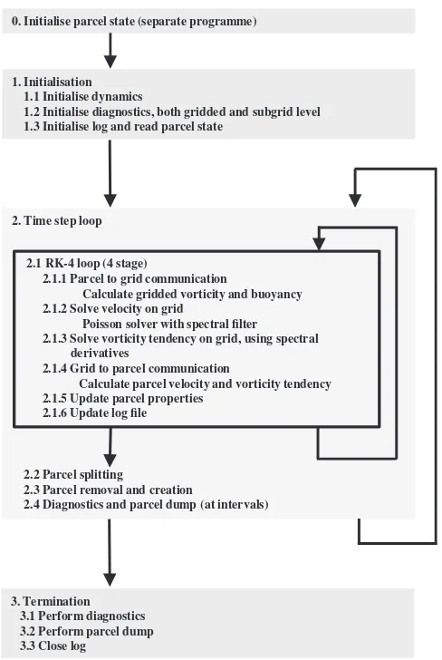
A schematic of the procedures comprising the MPIC algorithm is provided in Figure 1.
4 N U M E R I C A L T E S T S A N D P A R A M E T E R S E T T I N G S
We next examine the behaviour of the new MPIC model, in particular its dependence on numerical parameter set-tings, and illustrate how well the model compares with a state-of-the-art conventional numerical model (the focus of Böinget al., forthcoming). For this purpose, we study the evolution of a moist, initially buoyant thermal located near the ground level. The thermal rises at first through a neu-trally stable lower atmospheric layer before encountering a stable layer aloft. The initial fields of buoyancyb = bl and fractional specific humiditỹq= q∕q0are shown in Figure 2 together with a schematic of the background environment. Condensation (cloud formation) occurs once the thermal rises past the lifting condensation levelz= zc. The condensation
0.
1.
Initialise parcel state (separate programme)
2. Time step loop Initialisation 1.1 Initialise dynamics
1.2 Initialise diagnostics, both gridded and subgrid level 1.3 Initialise log and read parcel state
3.
2.2 Parcel splitting
2.3 Parcel removal and creation
2.4 Diagnostics and parcel dump (at intervals) 2.1 RK-4 loop (4 stage)
Termination 3.1 Perform diagnostics 3.2 Perform parcel dump 3.3 Close log
2.1.1 Parcel to grid communication
Calculate gridded vorticity and buoyancy 2.1.2 Solve velocity on grid
Poisson solver with spectral filter
2.1.3 Solve vorticity tendency on grid, using spectral derivatives
2.1.4 Grid to parcel communication
Calculate parcel velocity and vorticity tendency 2.1.5 Update parcel properties
[image:10.595.46.290.46.410.2]2.1.6 Update log file
FIGURE 1 A flow chart of the MPIC algorithm
acceleration, and takes the thermal past its level of dry neu-tral buoyancyz=zd. Only when the thermal encounters the level of moist neutral buoyancyz = zm (the nominal cloud
top) is the upward acceleration arrested. All these heights are defined in terms of a non-mixing parcel which does not over-shoot its height of neutral buoyancy. Throughout the evolution of the thermal, significant turbulent entrainment occurs (see below), so in fact only part of the thermal actually rises this far. The remainder becomes increasingly well mixed with the surrounding environment.
4.1 Non-dimensionalization
For convenience, we scale all variables in order to work with the fewest parameter combinations possible. Lengths are made dimensionless by taking the condensational scale height 1∕𝜆 = 1 in Equation 5. Time is made dimension-less by taking the characteristic squared buoyancy frequency
g𝜆Δ𝜃l0∕𝜃l0 = 1, whereΔ𝜃l0∕𝜃l0 = 0.01 is a characteristic
fractional variation of the liquid-water potential temperature. This gives a dimensionless gravity of g = 100. We scale the specific humidity qby its saturation value q0 at ground level (i.e. we use ̃q = q∕q0 in what follows), in terms of
which we obtain the following dimensionless expression for
the buoyancyb:
b=bl+bmmax
(
0, ̃q−e−z), (29)
where
bm = gLq0 cp𝜃l0.
(30)
Here, we take L∕cp = 2,500 K,q0 = 0.015 and 𝜃l0 =
300 K. This givesbm=12.5. In terms of the original,
dimen-sional value of gravity g, the buoyancy b is scaled by the characteristic valuegΔ𝜃l0∕𝜃l0, which is here 1% ofg.
4.2 Initialization
At the initial time t = 0, we place a spherical thermal of weakly varying liquid-water buoyancybland uniform (frac-tional) specific humiditỹq=̃qthadjacent to the groundz=0.
The thermal has radiusRand is centred atx= (Lx∕2,Ly∕2,R). To create an asymmetry in the subsequent evolution, we take
blof the form
bl=blth
(
1+ e1x
′y′+e2x′z′+e3y′z′
R2
)
, (31)
wherex′=x−L
x∕2,y′=y−Ly∕2 andz′=z−R, whilee1,e2
ande3are dimensionless constants. This preserves the mean value ofblas well as the centre of mass of the perturbation.
The environment around the thermal extending to the base of the stratified zone atz= zbis assumed to be well mixed,
withbl = 0 (without loss of generality) and having a uni-form specific humiditỹqenv a factor of 𝜇 times that in the
thermal, ̃qth. We specify the lifting condensation level zc, from which we obtain the specific humidity within the ther-mal:̃qth = exp(−zc). In turn, given𝜇, we obtain the specific humidity in the environment around the thermal:̃qenv=𝜇̃qth.
Next we specify the relative humidity h = hb at z =
zb. This, together with the environmental specific humidity,
determineszb throughzb = ln(hb∕̃qenv). Finally, we specify two further heights, the level of dry neutral stratificationzd
for the thermal, and the level of moist neutral stratification (the nominal cloud top)zm. From these values, we obtain the
thermal buoyancy
blth=N2(zd−zb), where N2=bme
−zc−e−zm zm−zd (32)
is the squared buoyancy frequency in the stratified zone. This follows from the requirements that (a) the thermal buoyancy matches the background stratification at z = zd (normally near or just above the condensation level zc), and (b) the total buoyancy at cloud topz = zmmatches the background stratification, i.e.
blth+bm
(
̃
q−e−zm)=N2(z
m−zd). (33)
(a) (b) (c)
FIGURE 2 Initial distributions of (a) liquid water buoyancybland (b) specific humidity fractioñqin a vertical cross-section cutting through the initial thermal. The basic-state stratification profile is shown in (c)
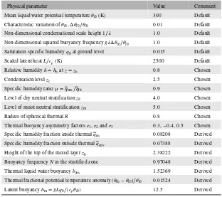
TABLE 1 List of physical parameters used in the simulations conducted. Units are included for dimensional quantities; all other quantities are dimensionless
Physical parameter Value Comment
Mean liquid water potential temperature𝜃l0(K) 300 Default
Characteristic variation of𝜃l0,Δ𝜃l0∕𝜃l0 0.01 Default
Non-dimensional condensational scale height 1∕𝜆 1.0 Default
Non-dimensional squared buoyancy frequencyg𝜆Δ𝜃l0∕𝜃l0 1.0 Default
Saturation specific humidityq0at ground level 0.015 Default
Scaled latent heatL∕cp(K) 2500 Default
Relative humidityh=hbatz=zb 0.8 Chosen
Condensation levelzc 2.5 Chosen
Specific humidity ratio𝜇=̃qenv∕̃qth 0.9 Chosen
Level of dry neutral stratificationzd 4.0 Chosen
Level of moist neutral stratificationzm 5.0 Chosen
Radius of spherical thermalR 0.8 Chosen
Thermal buoyancy asymmetry factorse1,e2ande3 0.3,−0.4,0.5 Chosen
Specific humidity fraction inside thermal̃qth 0.08208 Derived
Specific humidity fraction outside thermal̃qenv 0.07388 Derived
Height of the top of the mixed layerzb 2.38222 Derived
Buoyancy frequencyNin the stratified zone 0.97048 Derived
Thermal liquid water buoyancyblth 1.52369 Derived
Thermal fractional potential temperature anomaly(𝜃th−𝜃l0)∕𝜃l0 0.01524 Derived
Latent buoyancybm=gLq0∕(cp𝜃l0) 12.5 Derived
A full list of parameters used for the experiment conducted is provided in Table 1.
4.3 Default numerical parameter settings
For testing purposes, we consider a computational domain having side lengths Lx = Ly = 2𝜋 and a specified height
Lz(here also 2𝜋). This is large enough to accommodate the condensational scale height 1∕𝜆, here unity. The upper bound-ary has only a small influence until late times, t > 10. The domain is divided into equal-sized grid boxes, with side lengthsΔx=Lx∕nx,Δy=Ly∕nyandΔz=Lz∕nz. Here, with
Lx=Ly=Lzwe use an isotropic grid withnx=ny=nz=ng,
and choose ng = 128 as the default; other values are dis-cussed below and in Böinget al.(forthcoming). As discussed at the end of section 3, the time step Δt is adapted every
time step to be inversely proportional to the maximum vor-ticity magnitude, i.e.Δt = 0.5∕‖𝝎‖max. This relationship is
justified below by comparing both smaller and larger time steps (varying the prefactor 0.5 above). The only remaining numerical parameters are the dimensionless maximum par-cel stretch𝛾max (default 4) and the minimum parcel volume
fractionVmin̂ = Vmin∕ΔV (default 1∕63). Below, we discuss
the impact of varying these parameters about their default values.
4.4 Description of the flow evolution
[image:11.595.141.453.258.535.2]finer in each direction than the basic “inversion” grid (n3 g). In
fact any grid resolution could be used for the rendering, since the parcels alone determine the field values but, given our choice of the minimum parcel size, any finer rendering grid would produce a grainy appearance. Details of the rendering procedure may be found in Böinget al.(forthcoming).
Figure 3 illustrates a few stages in the flow evolution. Here we show the total buoyancyb, specific humiditỹq, condensed portioñqcof̃q(cloud amount), and the parcel vorticity mag-nitude‖𝝎‖, all in a vertical cross-sectionx = Lx∕2 slicing through the centre of the thermal initially (other views are similar). The parcel vorticity is shown in place of the total vorticity since the former can be obtained directly on a fine grid from the parcels and, moreover, dominates the resid-ual correction required to make the total vorticity solenoidal. The results shown compare closely with those obtained using the Met Office/NERC cloud model (MONC) run at more than double resolution (section 4.10 below and Böinget al., forthcoming).
At early times, the thermal deforms into a large vortex ring, forming a strong updraught near its centre and entraining air from the sides and below. This updraught is compensated by subsidence mainly around the outskirts of the ring (not shown). By timet=2, part of the thermal has pushed through the lifting condensation level at zc = 2.5 (corresponding to
z∕Lz ≈ 0.4 along the vertical axis) forming a small cap-like cloud. The cap-like cloud is partially environmental air that is pushed up by the actual thermal. The vorticity at this early stage is concentrated in a narrow zone near the edge of the thermal where horizontal gradients ofbare largest. As time advances, the thermal becomes progressively more turbulent, entraining and mixing more low humidity air (seẽqcatt=6 in particular). The vorticity partially collapses into a ring with an intense core att =4, then subsequently destabilizes and breaks down. This generates a multitude of billowing fine-scale structures reminiscent of actual cumulus convec-tion (e.g.̃qcatt = 4 in Figure 3). This process is described in detail in Grabowski and Clark (1993). The turbulence at the edge of a real cloud as it ascends is more intense than in this simulation, but is better captured at higher resolution (sections 4.9 and 4.10 below). By timet=6, part of the ther-mal reaches the level of moist neutral stratificationzm =5.0 (corresponding toz∕Lz ≈ 0.8), where it begins to spread out and gradually dissipate. By the end of the simulation att=10, the cloud has spread across most of the horizontal domain and contains much weaker updraughts and downdraughts (not shown).
This example serves to illustrate the rapid changes occur-ring on small scales within clouds as a result of variations in thermodynamic properties, as mentioned above. Modelling this complexity, both accurately and efficiently, is a severe challenge for any numerical model. We next examine how robust the MPIC model is in faithfully capturing the evolu-tion. In particular, we examine the dependence on various
numerical parameters, as well as on spatial and temporal resolution.
4.5 Dependence on maximum parcel stretch
We first examine the maximum parcel stretch𝛾max which is
used in Equation 20 to determine when a parcel should split into two. The greater the maximum parcel stretch, the longer a parcel stays intact. Here, we compare four values:𝛾max=2,
4 (the default), 8 and∞(for which splitting never occurs). In Figure 4, we qualitatively illustrate the dependence on𝛾maxby
comparing cross-sections of the total buoyancy fieldbin each simulation, at both an intermediate and a late time (t=4 and 8). All simulations are closely comparable, but the one with the smallest maximum stretch (𝛾max=2) exhibits the greatest
differences overall. Evidently, too frequent splitting causes numerical diffusion, removing small-scale features. On the other hand, the case with no parcel splitting (𝛾rmmax = ∞) is remarkably similar to the other two with moderate values of
𝛾max. Nonetheless, we argue that some parcel splitting is
nec-essary to more accurately resolve small-scale features, as well as to represent the effect of small-scale mixing integrated over the time evolution of the flow.
Differences between the simulations can be seen more clearly in the kinetic energy spectrum(k)and in the par-cel number densitypvol(V̂), shown in Figure 5 at the same times illustrated in Figure 4. The spectrum(k)is defined as the sum of (̂ûu∗ + ̂v̂v∗ + ŵŵ∗)∕2 over all wavevectors k whose magnitude |k|lies between k− 1∕2 andk+1∕2 (∗denotes complex conjugation). Also,pvol(V̂)dV̂ gives the
number of parcels having a volume fraction lying betweenV̂
andV̂+dV̂. In practicepvol is computed using finite-sized
binsΔV̂uniformly spaced in logV̂. In Figure 5, the case with the smallest𝛾max(=2, black curve) exhibits the greatest
dis-crepancies, with noticeably less kinetic energy at small scales (high total wavenumbersk). Likewise, the case with no split-ting (magenta curve) has significantly less kinetic energy at large and intermediate scales, and marginally greater kinetic energy at small scales. In the parcel number density, pvol,
we can see that the high maximum stretch case 𝛾max = 8
(red curve) struggles to produce small parcels. (The magenta curves remain unchanged since no parcels split in this case). The low maximum stretch case𝛾max = 2 (black curve)
pro-duces the greatest number of parcels, particularly at small scales as expected. Note that the fluctuations seen inpvolat larger volume fractions arise from splitting parcels by fac-tors of 2 together with the low sample size. The fluctuations diminish at later times (not shown) and are also weaker at higher resolution.
(a) (b) (c)
(g)
(d)
(e) (f) (h)
(k)
(i) (j) (l)
(o)
(m) (n) (p)
(s)
[image:13.595.59.538.46.553.2](q) (r) (t)
FIGURE 3 Time evolution of (a, e, i, m, q) total buoyancyb, (b, f, j, n,,r) specific humiditỹq, (c, g, k, o, s) nominal cloud amount̃qcand (d, h, l, p, t) parcel vorticity magnitude‖𝝎‖. Timetincreases downwards witht=(a–d) 2, (e–h) 4, (i–l) 6, (m–p) 8 and (q–t) 10. The fields in this and subsequent figures are shown in a vertical cross-section cutting through the centre of the domain atx=Lx∕2
(total) vorticity magnitude 𝜔max ≡ ‖𝝎‖max, and the
num-ber of parcels n(with log10 scaling) for four values of𝛾max
(these diagnostics are representative). Here, the case with no parcel splitting (magenta curve) has significantly lowerurms
and relatively high 𝜔max. This is found also for the large
maximum stretch case 𝛾max = 8 (red curve), albeit with a
smaller discrepancy inurms. The small maximum stretch case
𝛾max = 2 (black curve) compares closely with the default
case (𝛾max = 4, blue curve) forurmsbut shows much lower
values of 𝜔max. Collectively, these results, and others (not
presented) for𝛾max = 1.5, 3 and 6, indicate that our default
choice 𝛾max = 4 produces the least anomalous behaviour
overall.
4.6 Dependence on minimum parcel volume fraction
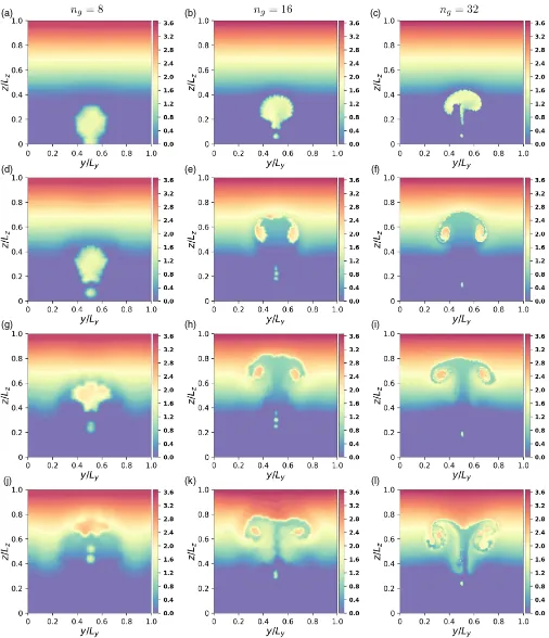
We next consider the effect of the smallest parcel size, spec-ified by the minimum volume fraction Vmin̂ . Three values are considered in Figure 7, namelyV̂min = 1∕4.53 (large),
1∕63(medium; default), and 1∕83 (small). Comparisons are