Synchronizing permutation groups and graph endomorphisms

(1)

AND GRAPH ENDOMORPHISMS

Artur Schaefer

A Thesis Submitted for the Degree of PhD at the

University of St Andrews

2016

Full metadata for this item is available in St Andrews Research Repository

at:

http://research-repository.st-andrews.ac.uk/

Please use this identifier to cite or link to this item: http://hdl.handle.net/10023/9912

(2)

Synchronizing Permutation Groups

and Graph Endomorphisms

A

RTUR

S

CHAEFER

T

HIS THESIS IS SUBMITTED IN PARTIAL FULFILMENT FOR THE DEGREE OF

P

H

D

AT THE

U

NIVERSITY OF

S

T

A

NDREWS

(3)

(4)

(5)

(6)

5

Abstract

The current thesis is focused on synchronizing permutation groups and on graph endo-morphisms. Applying the implicit classification of rank 3groups, we provide a bound on synchronizing ranks of rank3groups, at first. Then, we determine the singular graph endomorphisms of the Hamming graph and related graphs, count Latin hypercuboids of class r, establish their relation to mixed MDS codes, investigate G-decompositions of (non)-synchronizing semigroups, and analyse the kernel graph construction used in the theorem of Cameron and Kazanidis which identifies non-synchronizing transformations with graph endomorphisms [20].

The contribution lies in the following points:

1. A bound on synchronizing ranks of groups of permutation rank 3is given, and a complete list of small non-synchronizing groups of permutation rank3is provided (see Chapter 3).

2. The singular endomorphisms of the Hamming graph and some related graphs are characterised (see Chapter 5).

3. A theorem on the extension of partial Latin hypercuboids is given, Latin hyper-cuboids for small values are counted, and their correspondence to mixed MDS codes is unveiled (see Chapter 6).

(7)

described which are then applied to semigroups induced by combinatorial tiling problems (see Chapter 7).

(8)

7

Acknowledgements

I am very grateful for the funding provided by EPSRC and the School of Mathematics and Statistics which provided me with the chance to carry out this highly interesting research. I would like to thank the CIRCA group and its members for their inspiring meetings and talks, in particular Colva Roney-Dougal for her help and all the interesting discussions and James D. Mitchell for his help in GAP and semigroup issues.

I am immensely grateful to my excellent supervisors Nik Ruˇskuc and Peter J. Cameron for their help, advice and inspirations and support. In particular, I want to thank Peter for his interesting and challenging conversations. Moreover, I would like to thank Thomas Neukirch for his school related advice and morale and Collin Bleak for his advice and career related discussions. I would like to thank Feyisayo Olukoya (who has been one of the greates office mates ever), Casey Donoven and Sascha Troscheit for their interesting and fun chats. In particular, I want to thank them for the discussions which frequently occured on a Saturday in the office.

(9)

(10)

Contents 9

Chapter 1 Introduction

The Motivation

Synchronization has its origins in computer science, in particular, in the theory of deter-ministic finite automata (DFA). The concept of synchronizing automata has been around from the earliest days of automata theory in 1956 [12], but in his pioneering paper from 1964 ˇCern´y [22] was the first who explicitly mentioned synchronizing automata ( ˇCern´y called them directable automata; the term synchronizing did not appear until introduced by Hennie [42] in 1964).

A synchronizing DFA is an automaton admitting a sequence of transitions (or a word) which brings the automaton to a particular state no matter where it started. Such a word is called areset word; thus, a DFA is synchronizing, if it admits a reset word.

However, synchronizing automata have been reinvented several times over the years. This is due to the technological advancements and its technical applications of which robotics is one of the most important ones. For instance, industrial automation, loading, assembly and packing are common examples [79].

(15)

Figure 1.1: 4 possible orientations (cf. [79])

it needs to take a prescribed position, say upwards oriented, prior to assembly. Hence, there needs to be one spot on the conveyor belt where the parts are being rotated. Due to costs and simplicity, assume there are two robot arms at this spot applying the following two operations to the parts. Armarotates the part through90◦ (clockwise), only if it is left oriented and does nothing else; whereas armbrotates it through90◦(clockwise). The situation is described by the automaton in Figure 1.2, which turns out to be synchronizing. In his research, ˇCern´y found particular interest in the length of synchronizing words [22]. He developed a family of synchronizing automata containing a reset word of length at most(n−1)2. The previous example belongs to this family and the minimal length of a reset word is(4−1)2 = 9. Moreover, he conjectured that this bound holds for any synchronizing automaton (the first print version of the conjecture appeared in [23]).

Conjecture 1.1.1. A synchronizing automaton with n states contains a reset word of length at most(n−1)2_.

The conjecture has been proposed by various authors, and it has been verified for several partial cases (see [78] for an overview), but it remains unsolved for more than40

years. Thus, it is arguably one of the most long-standing open conjectures in the history of automata theory.

The main motivation for the current research comes from this conjecture, and is fur-ther motivated by the result of Trahtman [78] who verified the conjecture for aperiodic automata.

(16)

[image:16.595.225.371.86.236.2]

1.1. The Motivation 15

Figure 1.2: The automaton with reset wordab3_ab3_a_{(cf. [79])}

to the four states on which the transformations a and b act (given by the robot arms). Hence, S = ha, biis the corresponding submonoid. In general, a transformation semi-groupS ≤Tnis synchronizing if it contains a constant transformationi7→x, for a fixed

x∈ {1, ..., n}.

In this setting, an aperiodic automaton is a transformation semigroupS with a trivial subgroupG of permutations. Thus, the missing case in the ˇCern´y conjecture is where

S is a transformation semigroup of the form S = hG, Ti with non-trivial permutation groupG and T ⊆ Tn. So, in this thesis we are interested in semigroups of this form.

However, for synchronization purposes it is sufficient to consider semigroupshG, ti, for a single singular transformationt.

J. Ara´ujo was the first to tackle the case with non-trivial subgroupGof permutations [5]. He called a permutation groupGonnpoints synchronizing, if the semigrouphG, ti

(17)

1. Classify all synchronizing permutation groups, and

2. check whether the ˇCern´y bound is satisfied for each combination of synchronizing group and transformation.

Note, some ideas of how to check the second step can be found in [51, 11].

However, even the classification of all synchronizing permutation groups in this sim-ple looking approach turns out to be very difficult. So, to learn more about synchroniza-tion, non-synchronizing groups were considered. It was asked where such groups fail to be synchronizing; in detail, people looked for properties of transformations which fail to be synchronized, and it turned out that a particular rank of a transformation (size of its image) and uniformity (each kernel class has the same size) are good choices. So, the reader will notice that this research includes many discussions regarding ranks and uniformity of transformations.

A ground-breaking result in synchronization theory was achieved by Cameron and Kazanidis [20]. They gave an equivalence between transformations which are not syn-chronized and singular graph endomorphisms. Their theorem states that a permutation groupGdoes not synchronize a transformation tif and only if there is a non-trivialG -invariant graph with complete core which admitstas an endomorphism. Having a com-plete core means that the clique and chromatic number are identical, so this guarantees the existence of singular endomorphisms (cf. Lemma 2.3.3). Consequently, a permuta-tion group is synchronizing if and only if there is no non-trivialG-invariant graph with complete core. This resulted, for instance, in various theorems on ranks not synchro-nized, and this theorem is applied throughout this research.

(18)

1.2. The Current Research and Contributions 17

The Current Research and Contributions

The current thesis is focused on synchronizing permutation groups and on graph endo-morphisms, motivated by the theorem of Cameron and Kazanidis. Although it is not directly participating in the classification of synchronizing permutation groups, it tack-les various questions related to it. The problem most related to synchronizing theory is on ranks not synchronized by groups of permutation rank3; there we provide a bound on the ranks synchronized. Then, we determine the singular graph endomorphisms of the Hamming graph and related graphs, count Latin hypercuboids of classr, establish their relation to MDS mixed codes, investigate disjoint decompositions of synchroniz-ing semigroups, and analyse the graph construction used in the theorem of Cameron and Kazanidis.

This research is divided into 8 chapters, of which Chapter 2 constitutes the mathemat-ical background on the material covered here. Some parts of Chapter 2 have been moved to the appendix for a better comprehension. Afterwards, Chapter 3 introduces synchro-nization theory and proves a bound on non-synchronizing ranks of groups of permutation rank3. Moreover, it contains a list of small non-synchronizing permutation groups.

Subsequently, Chapter 4 gives many examples of non-synchronizing groups and anal-yses the corresponding endomorphism monoids. Also, here we provide a list of primitive and transitive graphs admitting a complete core and we count their singular endomor-phisms.

Afterwards, Chapter 5 provides a description of the singular endomorphisms of the Hamming graph. This chapter is the next main chapter of this thesis. Furthermore, three other families related to the Hamming graph are discussed, too. Also, the results on the Hamming graph are generalised to cuboidal Hamming graphs by mentioning so-called Latin hypercuboids of classr.

(19)

consid-ered. Then, in the context of Latin hypercubes we consider questions like extensions or completions of partial Latin hypercuboids, and determine their numbers for small values. In addition, we introduce mixed codes and define mixed MDS codes, and link mixed MDS codes to Latin hypercuboids of classr. At last, we discuss a construction of non-synchronizing semigroups from tilings. In particular, we consider the famous problem of tiling the chequerboard with dominoes. This construction will act as an important example in the next chapter.

Next, Chapter 7 introduces various notions of normalizing groups. This chapter is first of all extending the research in [3]. However, building on that the focus rapidly changes to various disjoint decompositions of non-synchronizing semigroups. The semigroups coming from tilings admit those decompositions, and many other non-synchronizing semigroups from Chapter 4, too.

(20)

19

Chapter 2 Mathematical Background

This introductory chapter covers the mathematical background necessary for this thesis; that is, the objects of interest and commonly used terms are defined, and notations and conventions are set. The four major topics covered in this chapter are permutation groups, transformation semigroups, graph theory and further combinatorial objects and results. First, permutation groups and transformation semigroups are introduced, and their ac-tions on the natural numbers are defined. Second, the basic graph theory notation is set and orthogonal arrays and Latin hypercubes are described.

(21)

Permutation Groups

Groups and Actions

Agroup Gis a set with a binary operation· : G×G → G, (g, h) 7→ g ·h satisfying the following axioms: (i) the operation is associative, (ii)G contains a unique identity element, and (iii) every element has a unique inverse.

Let Ω be a finite set. The symmetric group Sym(Ω) is the group consisting of all bijective maps onΩ, and its elements are calledpermutations. The image of an element

v ∈ Ω under a permutation g is denoted by vg. The set Ω is usually set to be n =

{1, ..., n}; soSndenotes the symmetric group onΩ.

Definition 2.1.1. Apermutation groupGof degreenis a subgroup ofSn

For technical reasons, we assume throughout this thesis thatGhas degree at least3. Cayley’s theorem states that every group can be represented as a permutation group. All groups considered in this thesis are permutation groups (if not explicitly mentioned), and the following example contains a list of popular groups and their various permutation representations, which can be found throughout this thesis.

Example 2.1.2. 1. The symmetric groupSnconsists of all permutations of{1, ..., n}.

2. The alternating groupAnis the set of all even permutations of{1, ..., n}.

3. The elements ofSncan also be represented as permutations of the2-sets of{1, ..., m},

wheren= m₂.

4. The wreath product Sk o Sm whose elements are permutations of the m-tuples

{1, ..., k}m_{, where}_n₌_km_{. (This is the primitive product action.)}

(22)

2.1. Permutation Groups 21

6. The affine general linear group AGL(d, q)can be represented as permutations of the points of ad-dimensional affine space over_Fq.

Now,Gacts onthe setΩif there is a homomorphism φ :G→ Sym(Ω). The image ofφ is a subgroup of Sym(Ω), and we usually writevg instead of v(gφ), when g acts on v. Given an action, the set vG = {vg : g ∈ G} is called the orbit of v under G. Moreover, the groupGistransitiveonΩif for any pairv, w∈Ωthere is a group element

g ∈ Gsuch thatvg = w. Equivalently,Gis transitive if and only if one of the orbits is the whole setΩ.

Transitive groups are well-known and constitute a very important part of group theory. However, if a group is non-transitive, then restricting its action to any of the transitive subsets provides a transitive action. In other words, the group is transitive on each of the subsets, and thus, the group can be seen as part of a Cartesian product.

Theorem 2.1.3. Any permutation groupGcan be embedded into the Cartesian product of transitive permutation groups, such thatGis a subcartesian product; that is,Gcan be mapped onto each factor under the natural projection map.

From now it is assumed that Gis transitive on Ω. LetB be a non-empty subset of

Ω, then B is called ablock (of imprimitivity)if for allg ∈ Gthe intersectionBg∩B is either empty orB itself. GactsprimitivelyonΩif the setΩand the singleton elements are the only blocks; otherwise, Gisimprimitive. Almost all groups in this research are primitive, and the remaining ones are transitive.

Primitive permutation groups are intensively studied in permutation group theory for the following reasons. Firstly, as transitive groups are the building blocks of a general group, primitive groups are the building blocks of transitive groups (by acting on each of the blocks of imprimitivity). Secondly, the next section presents the reduction theorem of O’Nan and Scott which subdivides primitive groups into classes. But, before this result is provided, more definitions are necessary.

(23)

Theorem 2.1.4. LetGact transitively onΩandGabe the stabiliser of a point. Then,G is primitive if and only ifGais a maximal subgroup.

The permutation rank of a transitive group G is the number of orbits of a point-stabiliserGa on the setΩ, wherea ∈ Ω(this is independent of the choice of a). Also,

this is equivalent to the number of orbits of Gon the tuples Ω×Ω[31, p. 67]. Next, the actions onk-subsets andk-tuples ofΩare described. A groupGisk-homogeneous

(ork-set-transitive) if it is transitive on thek-sets ofΩ. Similarly,Gisk-transitiveif it is transitive on the set ofk-tuples of distinct elements ofΩ. In particular, a 2-transitive group has permutation rank2, and we obtain the following implications, for|Ω| ≥3.

2-transitive⇒2-set-transitive⇒primitive⇒transitive.

The O’Nan-Scott Reduction Theorem for Primitive Groups

One of the main results on permutation groups is the O’Nan-Scott reduction theorem of primitive groups. The essence of this theorem is that primitive groups can be subdivided into finitely many classes according to their structure; however, there are various ways to choose these classes. For instance, in [65] the authors used five classes to classify the primitive groups, but following the approach of Cameron [19, Chapter 4] we are using only four classes.

In this subsection, we will solely provide this result and refer to Appendix A where the four classes are described in more detail. Also, this is where we define the socle of a permutation group.

Theorem 2.1.5(O’Nan-Scott). LetGbe a primitive group. Either 1. Gis non-basic; or

2. Gis basic andGis either of affine or diagonal type, orGis almost simple.

(24)

2.1. Permutation Groups 23

which are not relevant here, but which the reader can find in Cameron’s book [19, Thm. 4.7]. Moreover, using the classification of finite simple groups (CFSG) it is possible to subdivide the almost simple groups further into several subclasses.

Groups of Permutation Rank 3

One application of the reduction theorem and the CFSG is the classification of2-transitive and2-set-transitive groups (cf. [17, Lecture 2]). For instance, it follows that2-transitive groups are basic, but cannot be diagonal; a list of2-transitive groups can be found in [19]. However, another important consequence of this theorem is the classification of groups of permutation rank 3, which will be relevant to this research. If a primitive group has permutation rank3, then the following reduction is possible.

Theorem 2.1.6. IfGis a primitive group of permutation rank3, then either (A) Gis non-basic.

(B) G is non-abelian and almost simple whose unique minimal normal subgroup N

satisfies one of the following I) N is the alternating group, II) N is a classical group, or

III) N is an exceptional group of Lie type or a sporadic group. (C) Gis of affine type.

In case (A),Gis essentially a subgroup of the wreath productSnoS2 from Example

(25)

Example 2.1.7. The following are important examples from each of the three classes. (A) The wreath productSnoS2 acting on2-tuples.

(B) Snacting on2-sets.

(C) The1-dimensional affine groups GL(1, pd).

Semigroups

Basic Definitions

A semigroup S is a set of elements equipped with a binary operation · satisfying the associativity axiom(x·y)·z =x·(y·z), for allx, y, z ∈S. If, in addition,Scontains an identity element, thenSis amonoid. Semigroups are attracting more and more attention and this introductory chapter is not able to cover all the interesting properties of these objects, but instead we refer to other literature for a general inquiry; in particular, [45] and [56] contain very comprehensive introductory material.

However, the focus in this research is on finite transformation semigroups; that is semigroups given by maps from n to itself which, unlike permutations, do not need to be bijective. Hence, there arenn _{possible transformations on}_n_{, all included in the full}

transformation monoidTn. Therefore, the following definition is used.

Definition 2.2.1. Atransformation semigroupis a subsemigroup of the full transforma-tion semigroupTn.

Again for technical reasons, we assume throughout this thesis thatnis at least3. Similarly to Cayley’s theorem for permutation groups, any finite semigroup can be embedded intoTnfor somen.

(26)

2.2. Semigroups 25

Given a transformationt, therank oft is the size of its image im(t). However, the

rank of a semigroupS is something different; it is the size of a minimal generating set forS. IfScontains a subsemigroupGconsisting of permutations, thenS can be written asS = hG, Ti, whereT is a set of transformations. In this case the relative rank ofS

(with respect to G) is the minimal size of a set T such that S = hG, Ti. If the relative rank ofSis1, thenSis1-generatedorsimply generated. Furthermore,Sing(S)denotes the singular (non-bijective) maps inS; whereasE(S)denotes the set of its idempotents.

In this thesis, the following convention holds for writing transformations. A transfor-mationt mapping1to1,2to1and3to3, is represented by its dense image, i.e. by the listt= [1,1,3].

A non-empty subsetA ofS is aleft, right ortwo sided ideal ifSA ⊆ A, AS ⊆ A

orSAS ⊆ A. Consequently, every ideal is a subsemigroup, whereas the converse does not hold. Moreover, S1 _{denotes the monoid with an additional element, which is an}

identity inS. A transformation semigroup issimpleif it does not have any proper ideals. Hence, if S is simple with minimal ideal I, then S = I. Moreover, in the language of transformation semigroups the minimal ideal is the set of transformations of minimal rank.

A semigroupSisregularif every element ofSis regular, i.e. for alla∈Sthere is an

x∈S witha=axa. It iscompletely regularif every element is in some subgroup of the semigroupS. The theory of completely regular semigroups reveals that these decompose into subsemigroupsHi, for some indexi ∈ I, where everyHi admits a group structure

[45, Prop. 4.1.1]. Because the minimal ideal of a semigroup is simple, it is completely regular, too [45, Prop. 4.1.2].

Finally, a semigroup S is decomposable if it can be written as a disjoint union of subsemigroups.

Definition 2.2.2. Adecomposition of a semigroupS is a partition ofSinto at least two parts, where each partSi is a subsemigroup. Hence, S is the disjoint union S =

U

(27)

Green’s Relations

One essential structural feature of semigroups is given byGreen’s relations. These re-lations are equivalence rere-lations providing information about left, right and two-sided ideals of a semigroup, and are always of interest when encountering an unknown semi-group. In detail, two elementsa, bin a finite semigroupSare

• L-related if they generate the same principal left ideal, that isS1_a₌_S1_b_, • R-relatedif they generate the same principal right ideal, that isaS1 ₌_bS1_, • H-related if they areL- andR-related, and

• D-related if they generate the same principal two-sided ideal, that is

S1_aS1 ₌_S1_bS1_.

The equivalence classes of L-, R-, H- or D-related elements are called L-, R-, H- or

D-classes. Of particular interest are theH- andD-relations of regular semigroups, since several structural results are known (cf. [45, p. 45 ff.]), of which some are presented in Appendix C.

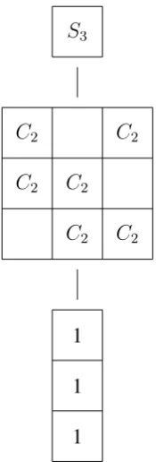
As already mentioned, calculating Green’s relations is one of the first calculations which should be applied to every new semigroup. These relations provide not only in-sights into the ideal structure of a semigroup, but also an overview of the interdependen-cies among the semigroup elements. A common way to visualise these relations is using egg box diagrams. These diagrams highlight the most important structural features at a single glance (see Figure 2.1). We refer to Howie’s book [45, p. 49] for the construction of eggbox diagrams.

Examples of Semigroups

(28)

2.2. Semigroups 27

1 1 1

C2

[image:28.595.254.342.83.342.2]

S3

Figure 2.1: Egg box diagram forT3

this thesis admit a particular kernel structure, i.e. the kernel classes have the same size, provided the semigroup contains a transitive subgroup of permutations. Transformations with such kernel structure are calleduniform, whereas non-uniform transformations have kernel classes of distinct sizes.

The simplest examples of semigroups not having a transformation of rank1are, pos-sibly, monogenic semigroups. Amonogenic semigroup is a semigroup S with a single generatora, namelyS = hai. Here asatisfies the equation am ₌ _am+r_{, for some}

non-negative integersmandr, wheremis theindexofaandritsperiod.

Some monogenic semigroups contain elements of rank1. In fact, inTna fraction1/n

of the elements (that is nn−1 elements) generate monogenic subsemigroups containing an element of rank1. This can be easily observed from Figure 2.2, where the rooted tree corresponding to the action oft= [1,1,2,2,3]on the set{1, ..,5}is given. Any transfor-mation generating a subsemigroup with an element of rank1is in1−1correspondence with a rooted tree, and there arenn−1_{rooted trees.}

(29)

commutativ-1

2

3 4

[image:29.595.217.378.87.243.2]

5

Figure 2.2: The rooted tree oft= [1,1,2,2,3].

ity holds, then this semigroup is asemi-lattice. However, left- and right-zero semigroups are of a different kind. A semigroup isleft-zeroif all elementsaandbsatisfyab=a; on the other hand, ifba=ais satisfied by all such pairs, then it is aright-zero semigroup.

Graph Theory

Basic Definitions

A graphΓ is a set of vertices V and edges E ⊆ V ×V. Starting with the adjacency relation, this section introduces terms from graph theory needed in this research. Because in this thesis undirected graphs are considered almost exclusively (and from now we consider undirected graphs only), v ∼ wmeans that the vertices v andw are adjacent. In this case, the vertexwis said to be aneighbour ofv, and vice versa. The number of vertices adjacent tovis thevalencyofv. In addition, if every vertex has the same valency

k, thenΓis calledregularof valencyk.

ApathinΓfromvtowis a list of verticesv =v1, v2, ..., vd=wsuch thatvi ∼vi+1,

fori= 1, ..., d−1. Γisconnectedif for any pair of verticesv andwthere is a path from

(30)

[image:30.595.238.363.89.169.2]

2.3. Graph Theory 29

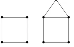
Figure 2.3: Both graphs admit a matching, whereas just the first one admits a perfect matching.

A matching in a graph is a set of edges without common vertices. Furthermore a

perfect matchingis a matching which covers all vertices (cf. Figure 2.3).

Graph Homomorphisms

For more details on the terms covered in the following subsection, we refer to [39, 41] and [38].

Definition 2.3.1. 1. Agraph homomorphismis a map which sends vertices to vertices such that adjacent vertices become adjacent vertices.

2. Anendomorphismof a graphΓis a homomorphism from this graph to itself. 3. AnautomorphismofΓis an endomorphism which is bijective and whose inverse is

an endomorphism, too.

The set of endomorphisms ofΓis a monoid and the set of automorphisms is a group so

End(Γ)stands for the endomorphism monoid andAut(Γ) for the automorphism group. Moreover, the set Sing(Γ) denotes the set (or semigroup) of singular endomorphisms, i.e.Sing(Γ) = End(Γ)\Aut(Γ).

A graph is symmetricif it has a non-trivial automorphism group Aut(Γ). If, in ad-dition, Aut(Γ) is transitive or primitive on the vertices V(Γ), then Γ is a transitive or

(31)

distance d(v, w) on a graph given by the length of the shortest path between two ver-ticesv and w, distance-transitive graphscan be defined, too. These are graphs whose automorphism group is transitive on ordered pairs of vertices at distancei, for alli. The

diameterofΓis the maximald(v, w)for distinct pairs of verticesv andw.

Next, colourings and cliques in graphs are defined. Ageneralised colouringofΓis (in the more modern sense) a homomorphism between two graphsΓand∆, namelyφ : Γ→

∆. Ak-colouringis a colouring where∆is the complete graphKk onk vertices. This

leaves room for further generalisations of graph colourings, for instance, other popular colourings are Kneser-colourings or circular colourings (see [39]). Similarly, acliqueof sizekinΓis a subgraph ofΓwhich is the complete graph onkvertices; this can also be regarded as a homomorphism, but this time fromKk toΓ. Thechromatic number χ(Γ)

is the smallestk such that there exists a homomorphism fromΓ to the complete graph

Kk; a homomorphism which is a χ(Γ)-colouring is usually called acolouring. On the

other hand, theclique numberω(Γ)is the size of the biggest clique inΓ. Moreover, the

co-clique numberα(Γ)denotes the clique number of the complementary graphΓ. The core of a graph Γ is a graph ∆ with the least number of vertices, such that there exist two homomorphisms, one fromΓ to∆ and another from∆to Γ. A simple characterisation of cores is given by automorphisms, namely, a graph is a core if and only if its endomorphisms are automorphisms. Cores of graphs are unique up to isomorphism. Furthermore, the core ofΓis the complete graph if and only if the chromatic number of

Γis equal to the clique number ofΓ.

Example 2.3.2. Examples of cores are the following: 1. odd cycles,

2. the complete graph and the null graph, which is the graph on n vertices without edges (those two graphs are calledtrivial graphsin this thesis),

(32)

(with16vertices and valency6) and the three Chang graphs (with 28vertices and valency12) (cf. Thm. 2.3.10). This can be easily checked in GAP [36].

Lemma 2.3.3. LetΓbe a graph whose clique number and chromatic number arer. Then, Γadmits endomorphisms.

Proof. Because those numbers are identical, there are homomorphisms

φ : Γ→Kr and ψ :Kr →Γ.

Thus,φ◦ψ : Γ→Γis an endomorphism.

In [20], the authors considered various classes of graphs coming from various combi-natorial structures and they realised that the core of most of those graphs admits a certain structure. In detail, the core is either the graph itself or it is complete; such a graph is called core-complete. Extending this research, Godsil and Royle [37] narrowed down the case where the core is complete. They defined the termpseudo-core, which denotes a graph that is either a core, or whose singular endomorphisms are colourings. This research deals with pseudo-cores and their endomorphisms.

Groups and Graphs

In this section, the interplay between permutation groups and graphs is introduced. If a permutation groupG acts onΩ, then the action on Ω×Ωinduces graphs. To see this, letObe an orbit under this action, then the graph induced byO is given byV = Ωand

E =O ⊆Ω×Ω.

(33)

and their pairs. Note that, we also sayG-invariant graphsto orbital graphs.

In this regard, we will need an additional definition. The2-closureofGis the set of all permutations ofΩwhich preserve theG-orbits onΩ×Ω. The groupGis2-closedif it is equal to its2-closure.

The above construction confirms that G is a subgroup of the automorphism group

Aut(Γ)of the graphΓ. Moreover, within this setting Higman was able to give another characterisation of primitive groups (cf. [19, Thm. 1.9]).

Theorem 2.3.4. A transitive group G is primitive if and only if all non-trivial orbital graphs are connected.

Strongly Regular Graphs

Strongly regular graphs admit even more regularity than regular graphs; astrongly regu-lar graphΓwith parameters(n, k, λ, µ)is a regular graph on nvertices with valency k

where

1. any two adjacent vertices have exactlyλcommon neighbours; 2. any two non-adjacent vertices have exactlyµcommon neighbours.

Many properties of strongly regular graphs are known (cf. [18, 38]); for instance, the diameter of a strongly regular graph is2. However, the strong regularity of the comple-ment graph is one of the most important ones. The parameters of the complecomple-ment graph

Γare denoted by(n, l, λ, µ)(sometimes we also writekforl.)

A characterisation of connected strongly regular graphs is given by the eigenvalues of its adjacency matrix. A connected regular graph is strongly regular if and only if it admits exactly three eigenvaluesk, rands[38, Lemma 10.2.1]. Indeed, one of the eigenvalues is the valency k. On the other hand, the graph n.Kr given by the disjoint union of n

complete graphs of sizeris the only non-trivial disconnected strongly regular graph, and

(34)

In this research we are mostly concerned with non-trivial strongly regular graphs, (i.e., graphs which are notn.Kr or its complement for any pair of non-negative integers

n and r). By using properties of the eigenvalues (see [18, Chap. 2]), we obtain the following result on the parameters ofΓ.

Lemma 2.3.5. IfΓ is a non-trivial strongly regular graph with parameters (n, k, λ, µ), then

k−µ≥ 1

3min(k, l). wherel =n−k−1is the valency of the complement ofΓ.

Proof. IfΓadmits the parametersn= 4µ+1andk = 2µ(which meansΓis a conference graph (cf. [18, pp. 110 & 38 ])), then k − µ = k/2 = l/2, thereby satisfying the conclusion. Otherwise the three eigenvalues k, r and s ofΓ (with r > 0 > s), are all integers, and in particularr≥1([49, p. 360 comment (A)]).

The parameters of a strongly regular graph can be expressed purely in terms ofk, r

ands(see [18, p. 39]) and from this it can be deduced that

kr(l+r+ 1)

k(r+ 1) +lr =

krs(r+ 1)(r−k)

k(k−r)(r+ 1) =−rs,

by substituting

l = k(k−λ−1)

µ =

−k(r+ 1)(s+ 1)

k+rs

into the left-hand side. From this, we can conclude that

k−µ=−rs= k(l+r+ 1)

k(1 + 1_r) +l ≥

                 l

2 + _kl ≥ 1

3l, forl ≤k,

k

2k_l + 1 ≥ 1

3k, fork ≤l,

(35)

Corollary 2.3.6. IfΓis a non-trivial strongly regular graph with parameters(n, k, λ, µ), then

k−µ≥ 1

3

√

n−1.

Proof. Because Γ and its complement are connected graphs of diameter 2, the well-known Moore bound [18, p45. Ex. 9] implies thatn ≤ k2 + 1 and n ≤ l2 + 1. The hypothesis follows from the previous result.

Over the past, various authors tried to characterise strongly regular graphs by their parameters, and surprisingly some graphs have been found to be uniquely determined that way. Because some of these graphs occur several times throughout this thesis, we give a definition and present their uniqueness results here (see Shrikhande and Chang [75, 24]).

Definition 2.3.7. 1. Thesquare lattice graphL2(n),n ≥3, is the graph whose vertex

set is the set of tuples overn, where two vertices are adjacent if exactly one of the two coordinates is identical.

2. Thetriangular graphT(n),n ≥5, is the line graph of the complete graph. 3. Thecocktail party graphCP(n),n ≥2, is the complementary graph ofn.K2.

Remark 2.3.8. 1. The square lattice graphL2(n)is equivalently the cartesian product

of Kn with itself (cf. Section 2.3.5) or the Hamming graphH(2, n)(cf. Chapter

5). Its automorphism group is the wreath product Sn oS2 with primitive product

action.

2. The automorphism group of the triangular graphT(n)is the symmetric groupSn

given by its representation on2-sets.

(36)

2. A strongly regular graph with parameters(1₂n(n−1),2(n−2), n−2,4), forn6= 8, is isomorphic to the triangular graphT(n).

Shrikhande has proved that forn = 4there is a distinct graph with the same param-eters as the square lattice graph; this graph is, nowadays, called theShrikhande graph. Similarly, Chang has shown that forn = 8 the three Chang graphs admit the same pa-rameters asT(8). In addition, various other graphs have been tested to have a unique set of parameters, too, for instance the Petersen graph, the Clebsch graph and the Schl¨afli graph.

The graphs just mentioned turn out to have one thing in common, namely the minimal eigenvalue. By a classification of Seidel (cf. [18, Thm. 4.14]), these graphs together with the cocktail party graphs are the only strongly regular graphs with minimal eigenvalue

−2.

Theorem 2.3.10(Seidel’s Theorem). A strongly regular graph with least eigenvalue−2 is one of the following:

1. the triangular graphT(n), n≥5,

2. the square lattice graphL2(n), n≥3,

3. the cocktail party graphCP(n), n≥2,

4. the Petersen graph,

5. the complement of the Clebsch graph,

6. the complement of the Schl¨afli graph,

7. the Shrikhande graph,

(37)

Rank 3 Graphs

IfGis a permutation group of permutation rank3, then the action ofGonΩ×Ωgenerates two non-trivial orbitsO1 andO2. The corresponding graphs are complementary graphs,

and are calledrank3graphs. This thesis is solely concerned with undirected graphs, and rank3graphs are undirected if, for example, the groupGhas even size.

Lemma 2.3.11. 1. A rank3graph is strongly regular.

2. IfGis a group of rank3and even size, then there is a rank3graph admittingGas subgroup of its automorphism group.

Note, from the classification of groups of permutation rank3we obtain (in theory) all rank3graphs.

Graph Products

The following two types of graph products occur frequently in this thesis.

Definition 2.3.12. LetΓand∆be graphs. Then, we define the following graph products on the vertex setV =V(Γ)×V(∆):

1. the Cartesian productΓ∆, where

E(Γ∆) ={((v, x),(w, y)) :eitherv=w,(x, y)∈E(H)orx=y,(v, w)∈E(G)},

2. the categorical productΓ×∆, where

E(Γ×∆) ={((v, x),(w, y)) : (v, w)∈E(G)and(x, y)∈E(H)}.

A small remark on this notation: The symbols and×originate from the products

(38)

2.4. Further Combinatorics 37

Further Combinatorics

Orthogonal Arrays and Latin squares

Orthogonal arrays have found much attention in the past, especially, when regarding codes; but many other applications are known. An extensive introduction to this topic and its various applications is found in [43].

Although, general orthogonal arrays which are covered in [43] are mentioned rarely, we still stick to this definition before restricting ourselves to the more special case with strength2and index1.

Definition 2.4.1. Anorthogonal arraywithn levels,kfactors, of strengthtand indexλ, i.e. at−(n, k, λ)orthogonal array, is ak×λnt_{array (matrix) whose entries come from} a set withnelements such that in every subset oftrows, everyt-tuple appears in exactly

λcolumns. In particular,OA(k, n)denotes an orthogonal array witht= 2andλ = 1.

ALatin squareis ann×n array with entries from ann-element set, such that every row and every column contains each entry precisely once. Moreover, two Latin squares are mutually orthogonal if after superimposition each of the n2 _{distinct tuples occurs}

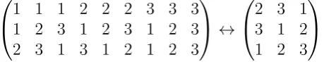
once. AnOA(3, n)orthogonal array represents a Latin square, where the three rows of the orthogonal array correspond to row number, column number and symbol of the Latin square (cf. Figure 2.4). So, a Latin square can also be considered as a set of triples. In general, a set ofk−2mutually orthogonal Latin squares (MOLS) can be identified with an orthogonal arrayOA(k, n), fork≥3.





1 1 1 2 2 2 3 3 3 1 2 3 1 2 3 1 2 3 2 3 1 3 1 2 1 2 3



↔





2 3 1 3 1 2 1 2 3



[image:38.595.184.414.675.719.2]



(39)

Latin Hypercubes of Class r

The definition of Latin hypercubes of dimension strictly greater than two is not obvious at all, because the extension is non-trivial and depends on several choices. The litera-ture provides different definitions of Latin hypercubes, where each construction has its advantages and disadvantages. In this research, we follow the approach of Kishen [53] who introduced Latin hypercubes of classr. This approach was adapted by Ethier [32] who provided various results on Latin hypercubes of classr, and, forr = 1, it leads to the Latin hypercubes defined by the two famous experts on Latin squares McKay and Wanless [67].

Definition 2.4.2. A Latin hypercube of dimension d, order n and class r is a

d-dimensional array with entries from a set of size nr _{such that in every} _r_-subarray each entry occurs exactly once. We write LHC(d, n, r) for such cubes (and sometimes LHC(d, n)instead of LHC(d, n,1)).

Example 2.4.3. The following is an example of a Latin hypercube of dimension3, order

3and class2. This cuboid has the top layerL1, middle layerL2 and bottom layerL3.

L1 =      

1 2 3 4 5 6 7 8 9

     

, L2 =      

5 6 4 8 9 7 2 3 1

     

, L3 =      

9 7 8 3 1 2 6 4 5

     

Two dimensional Latin hypercubes of class 1 are Latin squares; however, in this research we encounter further types of squares. A repetitive square is an n ×n array whose rows (or columns) are a permutation of the vectors

(1,1,1, ...,1),(2,2,2, ...,2), ...,(n, n, n, ..., n),

(40)

2.4. Further Combinatorics 39

Example 2.4.4. Two repetitive squares are the following:

           

1 1 1 1 · · · 1

2 2 2 2 · · · 2

3 3 3 3 · · · 3

..

. ... ... ... · · · ...

n n n n · · · n

            ,            

1 2 3 4 · · · n

..

. ... ... · · · ...

1 2 3 4 · · · n

            .

Now, we move to symmetry breaking of Latin hypercubes. A Latin square is in

reduced formif both its first row and first column are1, ..., n. It is calledsemi-reducedif the first row is1, ..., n, but not necessarily the first column. By permuting the rows and columns, every Latin square is similar to a reduced Latin square; however, this cannot be achieved for to higher classes (cf. Example 2.4.3). There, we need to stick to semi-reduced versions. That is, a Latin hypercube of class r is semi-reduced if the first r -subarray is naturally ordered with entries1, ..., nr_{. Every Latin hypercube of class} _r _is

similar to a semi-reduced one, and semi-reduced hypercubes simplify the calculations made in Chapter 6.

Hall’s Marriage Theorem

Hall’s marriage theorem is a very famous result in combinatorics and one of the key results in the theory of completions and extensions of Latin squares. Similarly, in this thesis we apply a modified version of this theorem to extensions of Latin hypercubes of classr(see Chapter 6). But before we get to that let us state Hall’s theorem.

(41)

Theorem 2.4.5(Hall’s Marriage Theorem). The setS admits a transversaltif and only if for every subsetX ⊆S, we have

|X| ≤ | [

A∈X

A|.

Our modified version of this theorem is given in terms of graphs. For this, we assume the setSis finite and contains the setsA1, ..., An. Then, define a bipartite graphΓwith

partsX andY as follows. LetX =SandY =

n

S

i=1

Ai. There is an edge betweenx∈X

andy∈Y if and only ify∈x. A transversal ofScorresponds to a matching inΓwhich covers all the vertices inX. However, we set a condition such that a perfect matching is produced. But before, an auxiliary theorem is needed.

Theorem 2.4.6(Dirac’s Theorem, Thm. 3 in [30]). A connected graph onnvertices with minimum valency n

2 has a Hamiltonian cycle.

Now, we come to the central result.

Theorem 2.4.7(Modified Hall’s Marriage Theorem). LetΓbe a bipartite graph on 2n

vertices whose parts X andY have n vertices each. If the minimal valency in Γ is at least n

2, then there exists a perfect matching inΓ.

Proof. Let the vertices inXbe setsA1, ..., Anand the vertices inY be elementsa1, ..., an,

where an element aj lies in Ai if the two vertices are adjacent. Hence, we are in the

situation of Hall’s theorem. Let L ⊆ X andR ⊆ Y its neighbourhood. As Γadmits a Hamiltonian cycle by Lemma 2.4.6, its restriction onL andR shows that |L| ≤ |R|. Thus, Hall’s theorem implies that there is a transversal forA1, ..., Anwhich corresponds

(42)

41

Chapter 3 Synchronization Theory

This chapter discusses the essentials of synchronization theory, its connection to per-mutation groups and graph theory, and the newest results on synchronizing ranks. The first sections lay the foundation for the following chapters regarding synchronizing semi-groups and synchronizing permutation semi-groups, and introduce the important equivalence between non-synchronizing transformations and graph endomorphisms. This equiva-lence provides a key technique in the analysis of synchronizing groups and is used fre-quently throughout this research.

The contribution in this chapter is given in the last section and provides bounds on the ranks of non-synchronizing transformations for groups with permutation rank3. Al-though, these results have already been published in joint work with Ara´ujo, Bentz, Cameron and Royle in [9], the bound has been considerably improved by the author.

Synchronizing Semigroups and Permutation Groups

(43)

permuta-tion groups is provided (cf. Neumann [69]), and synchronizing permutapermuta-tion groups are put into the context of other permutation group properties such as primitivity and 2 -transitivity.

Recall from Sections 2.1.1 and 2.2.1, we assume that the transformation semigroups and permutation groups we consider act on at least3points.

Definition 3.1.1(Synchronizing Semigroups). A transformation semigroup S ⊆ Tn is

synchronizingif it contains a transformation of rank1.

The main focus of this thesis lies on semigroups of the formhG, ti, for a permutation groupGand a singular transformation t. Hence, a synchronizing permutation group is defined as follows.

Definition 3.1.2(Synchronizing Groups). 1. A permutation group G synchronizes the transformationtif the semigrouphG, tiis synchronizing.

2. The groupGissynchronizingifGsynchronizes every singular transformationt.

Example 3.1.3. Cyclic groupsCp, for a primep, are synchronizing. This can be observed

directly, but it also follows from Corollary 3.3.8.

This definition provides a simple consequence for supergroups ofG.

Lemma 3.1.4. Any group containing a synchronizing subgroup is synchronizing.

The Main Problem in Synchronization Theory Motivated by Ara´ujo’s programme for tackling the ˇCern´y conjecture, the main problem in synchronization theory is the clas-sification of synchronizing permutation groups. Another significant and related problem is the classification of tuples(G, t)such that the corresponding semigrouphG, tiis syn-chronizing. In this thesis, we will tackle both problems.

(44)

3.1. Synchronizing Semigroups and Permutation Groups 43

namely by using section-regular partitions. Letπbe a partition of n = {1, ..., n}andσ

a subset ofn. The setσis asection(ortransversal) forπif it contains exactly one point from each part ofπ. In this regard, the partitionπis calledsection-regularfor the group

Gwith sectionσif the setσgis a section forπ, for all permutationsg ∈G. Equivalently,

πis a section-regular partition forGwith sectionσif the setσis a section for the partition

πg, for allg ∈G. This concept gives rise to the following equivalence.

Theorem 3.1.5. A permutation group Gis synchronizing if and only if there is no non-trivial section-regular partition forG.

Proof. A section-regular partitionπwith sectionσdefines an idempotent transformation

twith kernelπ and imageσ. Then, hG, tiis not synchronizing. Conversely, ifGis not synchronizing, then there is a transformationt of minimal rank not synchronized byG

whose kernel is a section regular partition with its image as the section.

Corollary 3.1.6. LetS =hG, tibe a non-synchronizing semigroup andf ∈Sof minimal rank. Then, the kernelker(f)is a section regular partition forGwith sectionim(f).

IfGis transitive, then the partitionπis necessarily uniform.

Lemma 3.1.7([69], Thm. 2.1). LetGbe transitive andπbe a section-regular partition forGwith sectionσ. Then,πis uniform.

The transformations induced by such a uniform section regular partition have uniform kernel, and thus they are calleduniform transformations. This property is crucial for the definition of almost synchronizing groups, later. However, next we place the synchroniz-ing property in line with other permutation group properties.

Lemma 3.1.8. 1. A2-set-transitive groupGis synchronizing. 2. A synchronizing group is primitive.

(45)

Proof. AssumeGis2-set-transitive, but not synchronizing; that is, there is a transforma-tiont of minimal rank r not synchronized by G. However, sinceG is 2-set-transitive, there is an element g ∈ G mapping two elements of the image oft to the same kernel class oft. Consequently, the elementtgthas rank< r; a contradiction.

Next assumeGis synchronizing but imprimitive, then any non-trivial partitionπfixed byGprovides a section-regular partition for any sectionσ.

Finally, assumeGis synchronizing and primitive, but not basic. Our goal is to provide a section-regular partition contradicting the assumption. As G is not basic, Ω can be identified with the coordinatesΓn_{for some set}_Γ_{. One possible partition is the following:}

Letπbe a partition ofΩaccording to the element ofΓfrom the first coordinate. So, in fact,πis a partition of the hypercubeΓninto hypercubesΓn−1(the cubeΓnis sliced into

nslices). Therefore, the diagonalσ ={(x, x, ..., x) : x ∈ S}acts as a section for every image ofπunderG. This is a contradiction to Thm. 3.1.5.

In consequence, the following implications are true for permutation groups.

2-transitive ⇒2-set-transitive⇒synchronizing⇒basic⇒primitive.

Graphs and Synchronizing Permutation Groups

A major breakthrough in the study of synchronizing permutation groups comes via a graph theoretical approach [20]. This result was found by Cameron and Kazanidis and works: If a group does not synchronize a transformationt, then t is a graph endomor-phism of a certain graph. In more detail, they defined the kernel graph Gr(S) for a transformation semigroup S on n points. This graph has vertex set {1, ..., n} and two verticesvandware adjacent if there isnotransformationt ∈Swithvt =wt.

(46)

3.2. Graphs and Synchronizing Permutation Groups 45

direct applications to synchronization theory.

Lemma 3.2.1. IfΓ =Gr(S), then the following hold. 1. S ≤End(Γ).

2. Γhas clique number equal to its chromatic number.

3. If S is synchronizing, thenΓis the null graph onn vertices, i.e. a graph with no edges.

4. IfSis a permutation group, thenΓis the complete graph.

Proof. Everything except for 2.is trivial. So, pick an element t in S of minimal rank

r. The image of t is a clique of size r in Γ, since t is minimal. But this means t is a homomorphism fromΓ to the complete graph Kr, which certifies that t is a colouring.

From Chapter 2 it is known that having clique number equal to chromatic number is equivalent to having a complete core. Moreover, endomorphisms of Gr(S) of minimal rank play an important role.

Corollary 3.2.2. IfΓ =Gr(S)is a non-trivial graph admitting a singular endomorphism of minimal rankr >1, thenχ(Γ) =ω(Γ) = r, and vice versa.

The key tool in synchronization theory is given by the next result which has a semi-group and a permutation semi-group version. First, the semisemi-group version is given.

Theorem 3.2.3. Let S be a transformation semigroup which is not a group. Then the following are equivalent:

1. S is not synchronizing,

(47)

Proof. The implication 3. ⇒ 2. is obvious and 2. ⇒ 1. follows from Lemma 3.2.1. SupposeSis not synchronizing. As before,Γ =Gr(S)is a non-trivial graph whose core is complete. Above, we have also verified thatS ≤End(Gr(S)).

The following is the permutation group version.

Theorem 3.2.4. A permutation groupGdoes not synchronize a mapf if and only if there is a non-trivial graphΓ, whose core is complete, such thatG≤Aut(Γ)andf ∈End(Γ).

Corollary 3.2.5. Gis non-synchronizing if and only if there is a non-trivial graphΓwith complete core, such thatG≤Aut(Γ).

Next, we have a look at the graph Gr(S) for a particular semigroup S. Let Γ be a graph with endomorphism monoid End(Γ). The hull of Γ is the graph Gr(End(Γ))

and is denoted by Hull(Γ). This graph plays a major role in the proofs of the previous theorems and in synchronization theory itself; so, Chapter 8 is dedicated to it. However, we present its basic properties here.

Lemma 3.2.6. LetΓbe a graph and∆ =Hull(Γ). Then, 1. Γis a spanning subgraph of∆,

2. ∆has clique number equal to chromatic number, 3. Aut(Γ) ≤Aut(∆),

4. End(Γ) ≤End(∆). In particular,

1. the null graph is a hull,

(48)

3.3. Synchronizing Permutation Groups 47

The hull turns out to be completing Γ or at least adding extra symmetry to Γ, as

Aut(∆)containsAut(Γ). In particular, the fourth property becomes important, but we will postpone it until Section 8.1 where we are going to highlight the advantages of graphs which are hulls.

Synchronizing Permutation Groups

Developing the Main Tools

In this section, the tools for the classification of synchronizing groups are developed. As mentioned above, Theorem 3.2.4 is currently the key tool in synchronization theory, so an algorithm for this classification is built around this theorem. But before we reveal it, we provide further auxiliary results.

The first of these results regards the isomorphism types of graphs.

Lemma 3.3.1. LetΓ1 andΓ2 be two graphs andφ : Γ1 → Γ2 an isomorphism. A map

f : Γ1 →Γ1 is an endomorphism ofΓ1if and only ifφ−1f φis an endomorphism ofΓ2.

Corollary 3.3.2. The groupAut(Γ1)is synchronizing if and only ifAut(Γ2)is.

The most simple case is whereGhas permutation rank3and even order. In this case there are just two complementary non-trivial orbital graphs.

Example 3.3.3. The group Sn, for n ≥ 5, has a primitive action on2-sets of

permuta-tion rank 3and the invariant graphs are the triangular graph T(n) and its complement. Furthermore,Snis synchronizing if and only ifnis odd [20].

In particular,S11acts on55points and the Mathieu groupM11acts on55points, both

as permutation rank3groups. However, there is only one connected non-trivial strongly regular graph on 55 points which implies that both graphs have to be isomorphic, and thusM11is also synchronizing.

(49)

Lemma 3.3.4. Let the groupGbe the2-closure of the permutation groupH. Then,Gis synchronizing if and only ifH is synchronizing.

Corollary 3.3.5. Let the groupsG1andG2have the same2-closureG(up to permutation

isomorphism). Then,G1 is synchronizing if and only ifG2is.

The above two “facts” are also true for primitivity and2-set-transitivity; so the syn-chronization property is in line with other permutation group properties. In addition, for vertex-transitive graphs another necessary condition is of major use (cf. [20]).

Lemma 3.3.6. LetΓbe a vertex-transitive graph onnvertices withω(Γ) =χ(Γ)(i.e.,Γ has a complete core). Then,ω(Γ)α(Γ) =n, whereα(Γ)is the co-clique number.

The Algorithm

This algorithm to classify the synchronizing permutation groups can also be found in [17]. It determines whether a group is synchronizing or not. Let G be a permutation group.

1. Compute all orbital graphs ofG(this is computationally fast);

2. Compute clique numberωand co-clique numberα(NP-hard, but very fast in prac-tice).

3. Compute the chromatic numberχfor every orbital graphΓwithω(Γ)·α(Γ) = n

(very hard, NP-hard). 4. Check ifω =χ.

Then,Gis synchronizing if and only if no graph withω =χis found .

(50)

3.3. Synchronizing Permutation Groups 49

However, the easiest case would be if this decision problem would be solvable by knowing the degree of the permutation group. Thus, in the next section we will discuss the role of the degree.

Synchronizing Degrees

Deciding if a group is synchronizing just by examining its degree would simplify the previous algorithm drastically. Unfortunately, such a result would be too good to be true. Still, we can not do it for all degrees, but at least for prime degrees and degrees of the form2p, forpprime.

Suppose the monoidhG, tiis non-synchronizing, whereGis a transitive permutation group. Then, it contains an elementf ∈ hG, tiof minimal rankr > 1, and as we have seen in the previous section the concept of a map of minimal rank is rather fruitful. In particular, sincef induces a uniform section-regular partition, r is a divisor of n. This provides the following simple observation.

Proposition 3.3.7. LetG be a transitive group of degreen with smallest prime divisor

p1, and letf be a map of rankr.

1. Ifr < p1, thenGsynchronizesf.

2. IfGis not synchronizing, then we can find a map admitting this by looking at ranks which are at mostn/p1 and dividen.

Proof. 1. By Corollary 3.1.6, a map of minimal rank not synchronized byGneeds to dividen.

2. Again, we search for maps of minimal rank not synchronized byG, where a witness of minimal rank has rank r ≤ n/p1. By the same corollary such a map needs to

dividen.

(51)

A similar result holds for groups of degree2p.

Theorem 3.3.9(Cor. 2.5,[69]). IfGis primitive of degree2p, thenGis synchronizing.

Computation: Non-Synchronizing Primitive Groups Of Small Degree

In Appendix E, all2-closed primitive non-synchronizing groups of degree less than (and including)100and all2-closed primitive non-synchronizing groups of permutation rank

3of degree less than630are determined.

Using the small primitive permutation groups library in GAP [36], we computed the representatives of each isomorphism class of 2-closed groups. Then, for each group we calculated the isomorphism types of all invariant graphs, and for each representative graph we checked whether it admits singular endomorphisms or not. If at least oneG -invariant graph admits singular endomorphisms, thenGis not synchronizing.

Almost Synchronizing Groups

In the previous section, the primitive non-synchronizing permutation groups of small degree were determined, and as can be seen from Appendix E there are various non-synchronizing groups.

One class of groups of particular interest is given by the automorphism groups of pseudo-cores. Godsil and Royle defined a pseudo-core to be a graph which is either a core or whose singular endomorphisms are colourings. Hence, if there are singular endomorphisms, then the automorphism group of such a graphΓwould synchronize all endomorphisms, except for the ones of rank χ(Γ) = ω(Γ). For instance, the square lattice graphL2(n), forn ≥ 3, and the triangular graphT(n), n ≥ 5, are pseudo-cores

(we justify that in Thm 4.1.1 and Section 4.2.1).

(52)

distin-3.4. Almost Synchronizing Groups 51

guishes primitive from synchronizing groups. In detail, it appeared that primitive groups synchronize all transformations except the ones with uniform kernel. This gave rise to the definition of almost synchronizing groups.

Definition 3.4.1. A permutation group is almost synchronizing if it synchronizes all transformations with non-uniform kernel.

Lemma 3.4.2. An almost synchronizing group is primitive.

Proof. Assuming the groupGis imprimitive, then the transformationt which collapses one block of imprimitivity into a single point and is the identity on all other blocks is not synchronized byG.

From the various examples of almost synchronizing groups, it was believed that all primitive groups are almost synchronizing (except for possibly finitely many groups). This was conjectured by Ara´ujo, and is stated as a problem in [7].

Conjecture 3.4.3. The primitive permutation groups are almost synchronizing.

So, from that moment the goal of several researchers was to prove this conjecture; and thus, in [7] the authors tackled this problem by providing the first families of groups satisfying it. However, it was believed that if the conjecture would be true, a classification of the synchronizing groups would be needed to prove it, which would brings us back to the original task (namely, the main problem of synchronization theory); but eventually, in [9] the authors provided sporadic counter-examples, as well as infinite families of counter-examples to this conjecture. This has led to two sub-problems. The first is the question of a classification of almost synchronizing groups [9, Problem 7.1]. The second is a relaxed version of the previous conjecture, and Remark 3.5.4 mentions a first result towards it.

(53)

A

D

E C

[image:53.595.231.365.88.159.2]

B

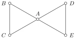
Figure 3.1: The butterfly

The smallest counter-example to the first conjecture is the primitive automorphism group of line graph of the Tutte-Coxeter graph. This group has degree45and admits a non-uniform graph endomorphisms whose image forms a butterfly (cf. Figure 3.1).

At the start of this research, this Conjecture 3.4.3 was still open and the aim of this thesis was to work towards a verification. The first place to look for a counter-example is the non-basic primitive groups; such a group is contained in the automorphism group of the Hamming graph. By that time it was already known that the Hamming graph admits uniform singular endomorphism of ranksnk_{, for}₁ _≤_k _≤ _m₋₁_{, where}_m _{is its}

dimension; however, Chapter 5 shows that all its singular endomorphisms are uniform. For the remainder of this section, we summarise the recent results on almost synchro-nizing groups. The groups considered next result are groups of permutation rank3.

Theorem 3.4.5(cf. [7]). 1. If Gis a subgroup of PΓL(n, q) containingP SL(n, q), wheren ≥5, acting on the lines of the projective space, thenGis almost synchro-nizing.

2. Let G be the semidirect product of the additive groups of _Fp2 by the subgroup

of index 2 in the multiplicative group of _Fp2, for p a prime. Then G is almost

synchronizing.

3. LetGbe the symplectic groupP Sp(4, q)or be obtained from it by adjoining field automorphisms, whereqis a power of2. ThenGis almost synchronizing.

(54)

3.5. Synchronizing Ranks 53

However, the following result generalises the previous theorem.

Theorem 3.4.6(see Roberson [72]). All strongly regular graphs are pseudo-cores. Hence, all groups of permutation rank3are almost synchronizing.

The next result is a consequence of the investigation undertaken in Chapter 5.

Theorem 3.4.7. Let G = SnoSm (with primitive product action) be the automorphism group of the Hamming graph. Then, form = 2and3the groupGis almost synchroniz-ing.

Proof. The groupG has permutation rankm+ 1; hence, form = 2 we have permuta-tion rank3. This case is covered by Theorem 3.4.6. However, for m = 3 we need to consider6non-trivial graphs. We see in Chapter 5 that all these graphs admit uniform endomorphisms.

The real problem arises when dealing with bigger values for m as the number of orbital graphs grows exponentially; however, more on this topic will be explained in Chapter 5.

Synchronizing Ranks

Primitive Groups and Synchronizing Ranks

In this section, we are concerned with the situation where a group does synchronize some, but not all transformations; and in particular, with the question, which ranks do the trans-formations not synchronized have? This problem is the first step towards a further analy-sis of the difference between synchronizing and non-synchronizing permutation groups, and one could say between primitive and almost synchronizing groups. The results here were also used to verify some cases of Ara´ujo’s conjecture on the equivalence of primitive and almost synchronizing groups.

(55)

· · ·

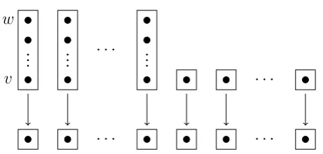
[image:55.595.229.373.83.190.2]

v w

Figure 3.2: Rystsov’s Theorem

Definition 3.5.1. Let G be a permutation group andr a positive integer. Then, r is a

synchronizing rank if G synchronizes all transformations of rank r; otherwise, r is a

non-synchronizing rank.

The first result on synchronizing ranks was established by Rystsov [73]. He provided a new characterisation of primitive groups using the means of synchronization, which is reproduced here.

Theorem 3.5.2(Rystsov). A transitive groupGof degree nis primitive if and only if it synchronizes every map of rankn−1.

Proof. IfGis imprimitive, then we form the complete multi-partite graph by assigning an edge to two vertices which are not in the same block ofG. The map which collapses all the points in one of the blocks forms a singular endomorphism of this graph which; so by theorem 3.2.4,Gis not synchronizing.

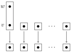
Conversely, assumeGis transitive andtis a map of rankn−1not synchronized by

G. Then, there is a graph Γ such that hG, ti ≤ End(Γ), by Theorem 3.2.4. Suppose

vt = wt, then v and w have the same set of neighbours, since each neighbour set is mapped bijectively to the neighbour set ofvt = wtbyt(see Figure 3.2). So, we define an equivalence relation by the following rule: v ≡ w if v and w have the same set of neighbours. This, relation isG-invariant and, thus,Gis imprimitive.

(56)

3.5. Synchronizing Ranks 55

the bound on synchronizing ranks of groups of permutation rank 3. The most recent results are as follows.

Theorem 3.5.3. A primitive groupGsynchronizes

1. every transformation of rankn−2,n−3andn−4. 2. every transformation of rank2.

3. every non-uniform transformation of rank3or4.

If, in addition,Ghas permutation rank3, then it synchronizes every map of rank bigger thann−(1 +√n−1/12).

Remark 3.5.4. Note that although the results on the ranksn−2, n−3andn−4hold for general primitive groups, the results on groups of permutation rank3are much stronger due to the additional structure provided by theG-invariant graphs, that is by their strong regularity. Moreover, this bound is a first result towards Conjecture 3.4.4.

Remark 3.5.5. During the final stages of this research the author learned of the pub-lication by Roberson [72] containing the result from Theorem 3.4.6. Result makes the bound from the previous theorem on groups of permutation rank3and the next section obsolete. However, the author decided to include the next section, since it contains the methods which have possibly some potential.

Groups of Permutation Rank 3

The Results

The result on groups of permutation rank 3 in the previous theorem originally comes from the research carried out in this thesis. However, due to its theoretical consequences and its similar methodology it has been published along with the results on ranksn−3