Bivariate Zero Inflated Power Series Distribution

(1)

Bivariate Zero-Inflated Power Series Distribution

Patil Maruti Krishna1, Shirke Digambar Tukaram2

1

Department of Statistics, P. V. P. Mahavidyalaya, Kavathe Mahankal, Sangli, India 2

Department of Statistics, ShivajiUniversity, Kolhapur, India E-mail: mkpatil_stats@rediffmail.com, dtshirke@gmail.com Received December 19, 2010; revised May 12, 2011; accepted May 15, 2011

Abstract

Many researchers have discussed zero-inflated univariate distributions. These univariate models are not suitable, for modeling events that involve different types of counts or defects. To model several types of de-fects, multivariate Poisson model is one of the appropriate models. This can further be modified to incorpo-rate inflation at zero and we can have multivariate zero-inflated Poisson distribution. In the present article, we introduce a new Bivariate Zero Inflated Power Series Distribution and discuss inference related to the parameters involved in the model. We also discuss the inference related to Bivariate Zero Inflated Poisson Distribution. The model has been applied to a real life data. Extension to k-variate zero inflated power series distribution is also discussed.

Keywords:Bivariate Zero-Inflated Power Series Distribution, Bivariate Zero-Inflated Poisson Distribution,

K-Variate Zero-Inflated Power Series Distribution

1. Introduction

In a manufacturing process there may exist several types of (say m) defects—for example, solder short circuits, solder voids, absence of solder etc. on one printed circuit board. These defects cause different types of product failure and generate different types of equipment prob-lems. In the above example there can be only one type of defect which occurs more frequently and the other de-fects occurs very rarely. Another situation could be both types of defects occur rarely and so on. To model several types of defects, multivariate Poisson model is one of the appropriate models to use. This can further be modified to incorporate inflation at zero and we can have multi-variate zero-inflated Poisson (MZIP) distribution. There are several ways to construct MZIP distributions. In the literature, Chin-Shang et al. [1] have discussed various types of MZIP models and investigated their distribu-tional properties. Deshmukh and Kasture [2] have stud-ied bivariate distribution with truncated Poisson marginal distributions. Gupta et al. [3] have considered inflated distributions at the point zero and studied the structural properties of the inflated distribution. Gupta et al. [4] have discussed score test for zero-inflated generalized Poisson regression model. Holgate [5] described the

es-timation of covariance parameter of bivariate Poisson distribution by iterative method. Lambert [6] considered zero-inflated Poisson regression model. Laxminarayana et al. [7] have studied bivariate Poisson distribution and the distributional properties of the model. Patil and Shirke [8] studied testing parameter of the power series distribution of a zero-inflated power series model. Patil and Shirke [9] also studied equality of inflation parame-ters of two zero-inflated power series distributions. It appears that majority of the study in the literature is re-stricted to Poisson distribution and its extension to mul-tivariate set up. Relatively less has been reported for the family of distributions containing other distributions.

(2)

2. Bivariate Zero-Inflated Power Series

Distribution

Let X and Y be two random variables with

probabil-ity mass functions





 

_{ }

1

1 1

,

x

a x P x

f

 



 and





 

2

2 2

,

y

b y P y

f

 





, .

x yT

where T is the common support of X and Y, ₁0,

2 0

  , a(.), b(.) 0 f₁

 

₁ 



a x

 

₁x ,

 

2 2

 

2 .

y

f  



b y 

Define,







 



 



 









 



 



, 1 2 1 1 2 2

1 1 2 2

, , , , , ,

1 X Y

P x y P x P y

g x E g X g y E g Y

    





 

 _   _, (2.1)

where, g₁

 

x and g₂( )y are bounded function on 2.

note that

We PX Y,



x y, ,  1, ,2



is a proper bivariate

distribution for a suitable choice of . Based on the distribution (2.1), in the following ntroduce three types of BZIPSD.

Type-I BZIPSD

we i

: When there is an inflation only at



x,y

  

 0,0 , we define the BZIPSD as











    



    

, 1 2

1 2

, 1 2

1 π π 0,0, , , , , 0,0 ,0 π 1

, ,π, , ,

π , ,π, , , , , 0,0

X Y

P x y

P x y

P x y x y

     

  

 _ _ _  _{ }

  

 

 



(2.2)

Type-II BZIPSD: When there is inflation at X component only, we define the BZIPSD as

(2.3)

Type-III BZIPSD: When there is inflation at component only, we define the BZIPSD as

(2.4)

In the present discussion we focus only on Type-IBZIPSD, re

Moment Generating Function

of (X,Y) is











    



    

, 1 2

1 2

, 1 2

1 π π 0, , , , , , 0,0 ,0 π 1

, ,π, , ,

π , ,π, , , , , 0,0

X Y

P y x y

P x y

P x y x y

     

  

 _ _ _  _{ }

  

 

 _



Y

-

 





  

 





, 1 2

1 2

, 1 2

1 π π ,0, , , , , 0,0 , 0,1, 2,

, ,π, , ,

π , ,π, , , , 0,1, 2, , 1, 2,3,

0 π 1

X Y

P x x y x x

P x y

P x y x y

     

  

 _ _ _  _

  

 



 



 

sults on the remaining two can be obtained analogously. The moment generating function













   



 





 







1 2

, 1 2

1 1 2 2 1 1 1 1 2 2 2 2

, ,

1 π π

t X t Y X Y

X Y

t X t Y

M t t E e

M t t

M t M t  E e g X M t E g X E e g Y M t E g Y

 

   

    _ _ _ _ _ _ _ _

(2.5)

Therefore, we have

 

M t M

 





 





 





1 , 1

1 1

2 , 2

2 2

, 0

1 π π

0,

1 π π

X X Y

Y X Y

t

M t

M t M t

M t

       

(2.6)

where MX

 

t1

 

j

f  and f_j







fj

 



 

denote

and MY

 

t2

m vari

are the moment generat-ing functions of rando ables X and Y of zero-

inflated power series distribution and M t1

 

1 and

 

2 2

M t are the moment generating functions dom

s having power series distribution with parame-ters 1

of ran variable

 and 2 respectively.

Su ose pp and

 

2

j f 





 respectively for This gives us

 



 

1, 2

j .



1 1

_{ }

1 1

f

E X M

f ₁

π

0

X

 



 



 

2 2

_{ }

 

2 2 2 π

0

Y

f

E Y M

f

 

  

 

 

_{ }

1

 

1 1

_{ }

 

1 2 1 1 1 1 1

1 1 1 1

π

( ) f

Var X f f

f f

 

 _ _ _

 

 _ 

 

 

  

 

(3)

 

_{ }

2

 

2 2

_{ }

 

2 2 2 2 2 2 2

2 2 2 2

π

( ) f

Var X f f

f f    _ _ _           _   _  _,

and the correlation coefficient is

   







  

 







 

  

 

_{ }

 

_{ }

 

1 1 1 1 1 1 2 2 2 2 2 2

1 1 2 2

1 2

2 2

1 1 2 2

1 1 1 2 2 2

1 1 1 1 1 2 2 2 2 2

1 1 2 2

π π

f e f e f f e f e f

e f e f

f f _f _f

f f f f

f f               _ _ _ _                _      _           _ _ _{ } _ _  _      _{ }     _  _ _{ } _   (2.7)

3. Estimation of the Parameters of BZIPSD

Let ,

 



X Yi, i



i1, 2,3, n be a random sample

ob-served from BZIPSD



π, , ,  ₁ ₂



. The likelihood function for the observed random sample is given by.

























1 2 1

π, , , ; , ,

i

a n

L    x y



  1 2 (3

1

1 2

1 π π 0,0, , ,

π , , , , i

XY i

a

XY i i

P

P x y

        



.1)

where if 0 and otherwise.

The co din unct ven by,

1 i

a 

rrespon



  

, 0,

i i x y 

g log likelihood f

0 i

a 

ion is gi

















1 2

0 1 2

lo ,

log 1 π π XY 0,0, , ,

n P

 

  





, 1 2

1 1

g π, , ; , ,

logπ log , , , ,

n n

i i X Y i i

i i

L x y

a a P x y



  

 









)

   (3.2

log 0 π L  

 , ₁

log 0 L   

 , ₂

log 0 L   

 and

log 0 L    

give the following equations.











0 , 0,0, , ,1 2

(1 π) π 0,0, ,

X Y a n P P        1

, 1 2

1 0 , π n i i

X Y 

 





 (3.3)

 

_

_









 

_

_





1 1

0 , 1 2

, 1 2

1 , 1 2

π 0,0, , ,

1 π π 0,0, , ,

, , , , 0 , , , , X Y X Y n

X Y i i i

i X Y i i n P

P

P x y

a

P x y

                   _    



_ (3.4)  

_

_





 

_

_





2 2

0 , 1 2

, 1 2

1 , 1 2

π 0,0, , ,

1 π π (0,0, , , )

, , , , 0 , , , , X Y X Y n

X Y i i i

i X Y i i n P

P

P x y

a

P x y

                    _  _  



 

_

_





 

_

_





0 , 1 2

, 1 2

1 , 1 2

π 0,0, , ,

1 π π (0,0, , , )

, , , , 0 , , , , X Y X Y n

X Y i i i

i X Y i i n P

P

P x y

a

P x y

                    _ _  



 (3.6)

where P  _{X Y}_, (.) denote _ PX Y, (.)

 

Solving Equations (3.3) to (3.6) simultaneously we get maximum likelihood estimators of the desired four pa-rameters. We note that all the four likelihood equations are non-linear in nature and do not have clo

lution. Now, we discuss a particular case namely BZIPD.

sed form of BZIPSD

4. Bivariate Zero-Inflated Poisson

Distribution

Let us set a x

   

 x!1, b y

   

 y!1, 1

 

x

g x e ,

 

2

y

g y e ,

 

1

1 1

f  e ,

 

2

2 2

f  e in the model

(2.1). Then we get BZIPD with probability mass func-tion.





   

(3.5)





 

















   

 

1 2 1 1 2 , , , 0,0 π 1 , , 0,0 where 1 1

x y

c

x y

P

1 2 1 2

1 π π 1 1 c 1 c

2 ( ) c ! ! X x Y y

x y e

e e e

x y

c e



  _ 



e   e e

e         x y   _ _       (4. 1

The moment generating function of (X,Y) is

(4.2)             )   _ _ 









 



 





 



 







1 2

1 1 2 2 0 0

1 1 2 2

1 π π , ,

1 .

t x t y

x y

e P x e P y

g x E g X g y E g Y

(4)

It is clear from the expressions of moment generating functions of X and that the marginal distributions

of X and Y are univariate zero-inflated power series dis-tributions with param ters

Y

e



π,1



and



π,2



respec-tively. Further we have

 

π 1 and

 

π 2

E X   E Y  

 





 

1 2



1 2





π 1 1 π

and π 1 1 π

Var X Var Y          

The correlation coefficient is turns out to be  





 







1 2

2   c

  1 2

2

1 2 1 2

1 1 π 1 π

c e            (4.3)

Remark 1: When there is no inflation , the cor-

 



π1



relation coefficient  is given by 2 1 2

1 2

c

c e  

 _     _, which coincides with the correlation coefficient given by Laxminarayan et al. [8]

Remark 2: If we choose g(.) to be an her

suit-able bounded function, we will have different form of BZIPD. Some other possible functions can be

 

z,

g z a 0 a 1; g z( )ez

0

etc.

Remark 3: If   , we get Bivariate Zero-Inflated Poisson distribution based on two independent random variables.

Estimation of the Parameters of BZIPD

Suppose



x y_i, _i



;i1, 2, , n is a random sample

ob-served from BZIPD



π, ,  ₁ ₂,



;i1, 2, , n. Then the likelihood function is given by



















 









1 2 1 2 1 2 1 2 1 2 1 ( ) 1 1 2 π, , , ; ,

(1 ) π 1 1 1

π 1 ! ! i i i i i i n a c c i a x y

x c y c

i i

L x y

e e e

e

e e e e

x y                _

_

                            



(4.4) where ai1 if



x yi, i

  

 0,

y ot 0 and otherwise.

The corresponding log likelihood is given by, ai 0 











 









_

_

 

1

 

2

 

1 1 1

log log log

i i i i i

i i i

a x  a y  a

  













 







1 2 1 2

1 2

1 2 0 1 2

1 1

log π, , , ; , log 1 π π 1 1 1 log(π)

! log ! log 1 i i

n n

c c

i i

n n n n n

x c y c

i i i i

i i

L x y n e e a a

x a y a e e e e

                                      



(4.5)

The mles of the parameters can be obtained equations e by solving and log 0 L    

in the followi

simultaneously. These equations are given ng: log ₀ π L  

 , 1 2

log 0 L   _  log 0 L   _  ,  



















 



1 2 1 2 1 2

1 π πe  1  1 1 2

0

1

1 1 1

0 π 1 n c c i i c c a e e e              

   1 

n e e

   



(4.6)   



 













 















_



_



_

1 2 2 1 1 2

1 2 1 2

1 2 1 2 ( ) 0 1 0 1

1 i _

π 1 1 1 1

1 π π 1 1 1

0 1 i i i c c c c n y c c

i i n i

i _x _c _y _c

n e c e e e e

e e e

a x _e _e _e

n n c a

e e e e

                                                          _



c c     (4.7)



 













 

























1 2 1 2 ₁ 1c ₁ e e

   2

1 2 1 2

2 1 1 2 ( ) 0 1 0 1 2

π 1 1

1 π π 1 1 1

0 1

i

i i

c c c

c c

n

x

c c

i i n i

i _x _c _y _c

i

n e c e e

e e e

a y _e _e _e

n n c a

e e e e

(5)



 









 























1 2 1 2 1 2 1 2

1 2

( ) 0

1

π 1 1

1 π π 1 1 1

0 1

i i

c c

x c y c

n

i _x _c _y _c

i

n e e e

e e e

e e e e

a

e e e e

   

 



   

   



 

    

   

 

 

    

 



of the marginal distribution of Y to ZIPD we get Chi square statistic = 0.6065 and P value = 0.4360. The table value of = 3.841. Therefore, ZIPD fits well for X_{and Y dat}

Thus now we can test whet BZIPD

(4.9)

From the above equations, it is clear that Equations (4.6) to (4.9) are non-linear in nature. Solving these equations is computationally cumbersome. Laxminara-yan et al. [7], adopt method of moments for the model without inflation parameter (i.e. ). In their model they have used estimates based on Method of Moment Estimators (MME), which coincide with Maximum Likelihood Estimators (MLE) of the marginal distribu-tions. This is not the case for the joint distribution. We have to solve four equations simultaneously in order to et the MLEs. In the following we obtain maximum like-lihood estimators for the following example and test for goodness of fit.

5. An Application

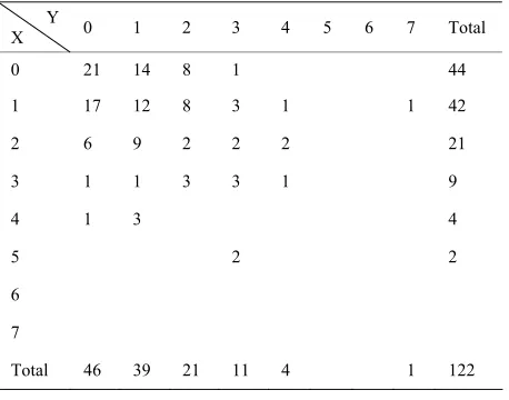
The data set in Table 1 reported by Arbous and Kerrich [10],

π1

g

represents accidents sustained by 122 railway men in consecutive periods of 6 and 5 years.

X is the accident distribution of 122 railway men dur-ing 1937-1942 and Y is the accident distribution of 122 railway men during 1943-1947.

By assuming marginal distributions of X is ZIPD



π,1



. The MLEs of X data are ˆπ0.8938 and

1

ˆ 1.2564

  Similarly assuming marginal distribution of Y is ZIPD



π,2



. The MLEs of Y data are ˆπ0.8494,

2

ˆ _1.3221

[image:5.595.78.287.81.156.2]

  _{. Using these mles we fit the data of the} mar-ginal distribution of X to ZIPD, we get Chi square statis-tic = 0.74843 and P value = 0.3869. If we fit the data Table 1. Bivariate accident distribution of 122 railway men

0 1 2 3 4 5 6 7 Total during two periods.

Y X

0 21 14 8 1 44

1 17 12 8 3 1 1 42

9

5

2 6 9 2 2 2 21

3 1 1 3 3 1

4 1 3 4

2 2

6

7

Total 46 39 21 11 4 1 122

2 (1,0.05) 

a.

her data is coming from



π, , 1 2



.

n (4.5) using m likeliho

0

Maximizing the log likelihood in the

Equatio MATLAB R12 software we get

maximu od estimators of the parameters as

π0.94 ,  1 1.210,  2 1.20,  1.220 -Inflated

. With

Zero Poisson

Distribution to the above data. The expected frequencies are as shown in the Table 2.

From the chi-square good

calculated , is less than the table value of alue is 0.392369. Hence we

o-Inflated Poisson Distribu-tion fits well for the data.

Remark 4: There can be m ny ways to define k

-vari-A k-variate Zero-Inflated Power Series Distribution ca b e ed

these parameters we fit Bivariate

ness of fit, we observed that

2 _4.102062

 

9.488. The P v hat Bivariate Zer 2

(4,0.05)

 

conclude t

a

ate ZIPSD by extending the above defined BZIPSD. One of the ways is given below.

n e d fin as

















1 π π , , f 0

,

, f

X

P x P x 

 

i ,π

πP x, i x 0

X   x

  

 

 

where





1, , ,2 k



    _, X 



X X₁, ₂,X_k















 







, ,

i

X

X i i

P x

P x g E g X



  

 _  _

 



i



1 1

i

k k

i i

x



,



i

X i i

P x 

ries Distri uti

is probability ma fu cti of ow r Se-o

In ted to parameters involved in

m an a p si arly.

modat

ons. Further work under consideration is te

model fo

≥2 Total

ss n on P e

b n. ference odel c

rela be

the ted

this

ttem mil

In the present work we introduced a new bivariate zero-inflated power series distribution. This distribution can accom e number of zero-inflated bivariate dis-crete distributi

sting of independence for BZIPSD. Application of the proposed r some other distributions like Bivari-ate Zero-InflBivari-ated Negative Binomial Distribution or k-variate zero inflated Poisson distribution can also be

Table 2. Expected frequencies using BZIPD.

Y

X 0 1

0 21.1914 11.5500 8.7747 41.5161

1 11.6746 15.1344 14.5680 41.3770

≥2 8.9933 14.7627 15.3421 39.0981

[image:5.595.59.288.546.726.2] [image:5.595.306.537.628.721.2]

(6)

[1] L. Chin-Shang, K. Kyungmoo, J. P. Peterson and P. A. Brinkley, “Multivariate Zero-Inflated Poisson and Their Applications,” Technometrics,Vol.41, No. 1,

99, pp. 29-38.doi:10.2307/1270992

doi: 10.1081/STA-120026576

considered. These models are useful to model

zero-in-flated bivariate data. [5] P. Holgate, “Estimation for the Bivariate Poisson

Distri-307/1269547

6. References

Models

19

[2] S. R. Deshmukh and M. S. Kasture, “Bivariat

tion with Truncated Poisson Marginal Distributions,”

Communication in Statistics: Theory and Metord

31, No. 4, 2002, pp. 527-534.

doi:10.1081/STA-120003132

e

Distribu-s, Vol.

[3] P. L. Gupta and R. C. Tripathi, “Inflated Modified Power Series Distributions with Applications,” Communication in Statistics: Theory and Metords, Vol. 24, No. 9, 1995,

pp. 2355-2374.doi:10.1080/03610929508831621

[4] R. L. Gupta and R. C. Tripathi “Score Test for Zero- Inflated Generalized Poisson Regression Model,” Com-munication in Statistics: Theory and Metords, Vol. 33,

No. 1, 2004, pp. 47-64.

bution,” Biometrika,Vol. 51, No. 1-2, 1964, pp. 241-245. [6] D. Lambert, “Zero-Inflated Poisson Regression, with an

Application to Defects in Manufacturing,” Technometrics,

Vol. 34, No. 1, 1992, pp. 1-14.doi:10.2

[7] J. Lakshiminarayana, S. N. N. Pandit and K. Srinivasa Rao, “On a Bivariate Poisson distribution,” Communica-tion in Statistics: Theory and Metords, Vol. 28, No. 2, 1999, pp. 267-276.

[8] M. K. Patil and D. T. Shirke, “Testing Parameter of the Power Series Distribution of a Zero-Inflated Power Series Model,” Statistical Methodology,Vol. 4, No. 4, 2007, pp.

393-406.doi:10.1016/j.stamet.2006.12.001

[9] M. K. Patil and D. T. Shirke, “Tests for Equality of Infla-tion Parameters of Two Zero-Inflated Power Series Dis-tributions,” Communications in Statistics: Theory and Methods, Vol. 40, No. 14, 2011, pp. 2539-2553.

doi:10.1080/03610926.2010.489172

[10] A. G. Arbous and J. E. Kerrich, “Accident Statistics and the Concept of Accident Proneness,” Biometrics, Vol. 7,