Neural Modeling of Multivariable Nonlinear Stochastic System Variable Learning Rate Case

doi:10.4236/ica.2011.23020 Published Online August 2011 (http://www.SciRP.org/journal/ica)

Neural Modeling of Multivariable Nonlinear Stochastic

System. Variable Learning Rate Case

Ayachi Errachdi, Ihsen Saad, Mohamed Benrejeb

Unit of Research LARA Automatic, le Belvedere, Tunisia

E-mail:[email protected], [email protected], [email protected] Received December 23, 2010; revised January 20, 2011; accepted January 27, 2011

Abstract

The objective of this paper is to develop a variable learning rate for neural modeling of multivariable nonlinear stochastic system. The corresponding parameter is obtained by gradient descent method optimiza-tion. The effectiveness of the suggested algorithm applied to the identification of behavior of two nonlinear stochastic systems is demonstrated by simulation experiments.

Keywords: Neural Networks, Multivariable System, Stochastic, Learning Rate, Modeling

1. Introduction

The Neural Networks (NN) was well used in modeling of nonlinear systems because of its ability of learning, its generalization and its approximation [1-4]. Indeed, this approach provides an effective solution for wide classes of nonlinear systems which are not known or only partial state information is available [5].

Identification is the process of determining the dy- namic model of a system from measurements inputs/ outputs [6]. Often, the measured output system is tainted noise. This is due either to the effect of disturbances act-ing at different parts of the process, either to measure-ment noise. Therefore these noises may introduce errors in the identification. The stochastic model is a solution to overcome this problem [7]. In this paper, a multivariable nonlinear stochastic system is our interest.

Among the parameters of the NN model, the learning rate ( ) has an important role in training phase. In this phase several tests are taken account to find the suitable fixed value. For instance, this parameter can slow down this phase of training [8,9] if it is small. However, if this parameter is large, the training phase is occurring quickly and it becomes unstable [8,9]. To overcome this problem, an adaptive learning rate was asked in [8,9]. This solu- tion is applied in training algorithm of a nonlinear sin- gle-variable system [8] and in multivariable nonlinear system [9]. In this paper, a variable learning rate of neu- ral network is developed in order to model a multivari- able nonlinear stochastic system. Different cases of sig- nal ratio to noise (SNR) are taken account to show the

influence of the noise in identification and the stability of training phase.

This paper is organized as follows. In second section, a multivariable system modeling by neural networks is presented. In third section, the fixed learning rate method is showed. The simulation of the multivariable stochastic systems by NN method using fixed learning rate is de- tailed in the fourth section. The development of the variable learning rate and results simulations are pre- sented in fifth section. Conclusions are given in sixth section.

2. Multivariable System Modeling by Neural

Networks

To find the neural model of such nonlinear systems, some stages must be respected [10]. Firstly the input variables are standardized and centered. Then, the struc- ture of the model is chosen. Finally, the synaptic weights are estimated and the obtained model must be validated. In this context, different algorithms are interested of the synaptic weights estimation. For instance, the gradient descent algorithm [11], the conjugate gradient algorithm [11], the one step secant [11], the Levenberg-Marquardt method [11] and resilient Backpropagation algorithm [11] are developed and confirmed their effectiveness in train- ing. In this paper, the gradient descent algorithm is our interest.

1 ,

N

il

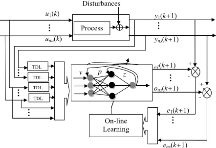
model [12], that is given by the Equation (1). The archi- tecture of the RNN is presented in Figure 1.





 





 





2

1

1 , ,

, , 1

i p i i

i i

y k f y k y k n

u k u k n

  _  

  



 (1)

The output of the hidden node is given by the following equation: th l 1 2 1

, 1, ,

N

l lj j

j

h p v l







 _ (2)

The neural output is given by the following equa-tion: th i





 

2 1 2 1 1 1 1

, 1, ,

N N

i lj j

l j

N

l il l

o k f f p v z

f f h z i ns

           _   _        _{ }  

 



   

1 _

  

(3)

Finally, the compact form is defined as:













 

 

 

 

 

   

2 2 2 2 1

1 _{11 1}

1 1 1 1 1 ... ns N _ns N nsN N T o k O k o k

f h f h _{z z}

f

z z

f h f h

f Z k F P k v k             _     _{  }  _{  }     _  _{ } _  _       _ _ _           (4) where

 

 

 

 

 

1

2 2 1 1

2 11 1 1 1 ... N

N N N N

N

T

p p

f h v k

f

p p v k

f h F Pv   _{    }   _{    }  _{      }   _{    }              

The principle of neural modeling of the multivariable stochastic system is showing in Figure 1.

To show the influence of disturbances on modeling, a noise signal is added to the output system. Dif- ferent cases of Signal Noise Ratio (SNRi) are taken. This

(SNRi) measures the correspondence between the system

output and the estimated output, the equation of is as follows:

 

i b k i SNR

 





 





0 0 1 1 N i i k i N i i k

y k y N

SNR

b k b N     





(5)

unu(k)

-+

-+

ens(k+1)

e1(k+1) ons(k+1) o1(k+1)

yns(k+1)

y1(k+1) Disturbances

u1(k)

On-line Learning

z

v p

Process

[image:2.595.313.534.79.230.2]

TDL TDL TDL TDL

Figure 1. Principle of the neural modeling of the multivari-able stochastic system.

The accuracy of correlations relative to the measured values is finding by various statistical means. The criteria exploited in this study were the Relative Error (RE), Root Mean Square Error (RMSE) and Mean Absolute Percentage Error (MAPE) [11] given by :







₂



1 2 2

i i i

REE_ y o y _

  (6)

 

 

 

0 100 N i i k i

MAPE e y k o k

N 





 (7)

3. Fixed Learning Rate Method

The neural system modeling is the research of parame- ters (weights) model. The search of these weights is the subjects of different works [1-6,8-13]. The gradient de- scent method is one among different methods which was well applied on neural identification for single-variable system [8] and for multivariable system [9]. In this paper, the same principle is suggested to be applied on neural identification of the multivariable stochastic systems. Indeed, the _ith criterion is minimized as follows:

 

1



 



2 1

 

 

2

2 2

i i i i

J k  e k  _y k o k _ (8) By application of the GD method, the theory of [1] is used; we find then [9]:

 For the variation of the synaptic weights of the hidden layer towards the output layer with



i1, ,_ ns



.

 

 

 

   

i i

il i i i

il il

J k o k

z e

z k z k

   

   

  k (9)

The compact form (4) is used here, so we find

 



_{ }

 



 

     

'

T il

il i l i

il

i l i

z F Pv

z f h e

z k

f h F Pv e k

Finally, the synaptic weights of the hidden layer to- wards the output layer can be written in the following way:

 



1



     

il il i l i

z k z k  f h F Pv e k (11)

 For the variation of the synaptic weights of the input layer towards the hidden layer.

 

 

 

   

 



_{ }

 



 

   

 

i lj i lj i i i lj T il

i l i

lj T

i l il i

J k p p k o k e k p k

z F Pv

f h e

p k k

f h F Pv z v e k

                   (12)

Finally, the synaptic weights of input layer towards the hidden layer can be written in the following way:

 



1



       

lj lj i l il i

p k p k  f h F Pv z k e k (13) In these expressions, i is a positive constant value

[8,9] which represents the learning rate (0 i 1) and

 

F Pv represents Jacobian matrix of F Pv

 

T

.

 

1

1, , 2

1 l N

N lj j j

F Pv diag f p v

       _ _{ }    



  (14) 1 1 1 2 1 1

1 _{1, ,}

N lj j N

j

lj j _N

j

lj j j

l N

f p v

f p v

p v    _        _{ }       _{ }   







 (15)

4. Simulation of Multivariable Nonlinear

Stochastic Systems

(

SNR



5)



In this section, two types of multivariable nonlinear sto-

chastic systems with 2 dimensions are

presented with . The system



[8] and [14] are defined respectively by the following equations:



nu2,ns2





1

S



SNR5

 

S2

 





 



 





 





 





 





 



 





 

 

1 1 1

1

1

1 1 1

2 2 2

2

1 2

1 0.3 0.6 1

0.6sin π

+0.3sin 3π

0.1sin 5π

1 0.3 0.6 1

0.8sin 2 1.2

y k y k y k

u k

u k

S u k b k

y k y k y k

y k

u k b k

                     _   _{ } 

 





 

_{ }

   

 





 

   

_{ }



 



 

1 1 3 2 2 1 2 2 1 2

1 1 2 1

2 2 2 2 0.8 1 2 0.8 1 2

y k u k u k

y k

y k

b k S

y k y k y k u k

y k y k b k         _      _{ }  _   _   (17)

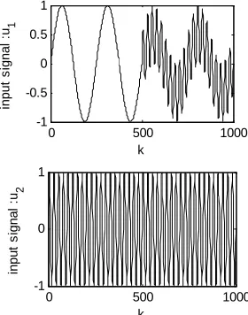
with 1 and 2 are a random signals, or u1 and 2 are the input signals of the systems considered defined by:

b b u

 

1 2π sin 250 k u k  _

 



 (18)

and

 

2 2π sin 25 k u k  _

 



 (19) The input signal and are presented in Figure 2.

1

u u₂

4.1. Simulation Results of System (S1)

A dynamic NN is used to simulate a multivariable nonlinear stochastic system (S1)



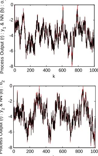
. In Figure 3, the evolution of the process output and the NN output of the system (S1) is presented. The estimation error be- tween these two outputs is presented in Figure 4.



SNR5

The obtained results, present that for a fixed learning rate ₁0.32, the NN output ₁ follows the measured output ₁ with an error of prediction and that ₂ follows the measured output ₂ with an error of prediction o y o e 1 0.0720 e  y

20.0601whose learning rate is 2 0.27

  .

0 500 1000 -1 -0.5 0 0.5 1 input s ignal : u1 k

[image:3.595.352.492.511.689.2]

0 500 1000 -1 0 1 in p u t s ig n a l :u 2 k





(16)

0 200 400 600 800 1000 -8

-6 -4 -2 0

k

P

roc

es

s

O

ut

put

(

r)

:

y1

&

N

N

(b

) :

o1

0 200 400 600 800 1000 -8

-6 -4 -2 0

P

roc

e

s

s

O

u

tput

(

r)

:

y2

&

N

N

(

b

) : o

2

[image:4.595.99.246.78.321.2]

k

Figure 3. Output of process and NN of system (S1) using a fixed learning rate.

0 200 400 600 800 1000 -0.1

0 0.1

L

ear

ni

n

g E

rr

or

:

e1

k

0 200 400 600 800 1000 -0.1

0 0.1

Le

ar

n

ing

E

rr

o

r :

e2

[image:4.595.351.497.81.321.2]

k

Figure 4. Learning error between the output of process and NN.

If this system has not an added noise, the error of pre-diction is e10.0384 and e20.0375 [9].

4.2. Simulation Results of System (S2)

A dynamic NN is used to simulate a multivariable nonlinear stochastic system (S2)



. In Figure 5, the evolution of the process output and the NN output of the system (S2) is presented. The estimation error be- tween these two outputs is presented in Figure 6.



SNR5

The obtained results showing in Figure 5, present that for a fixed learning rate 10.3, the NN output o1 follows the measured output 1 with an error of predic-tion 1 and that o2 follows the meas- ured output with an error of prediction

y 0.0650

e 

2

y e₂0.0670

0 500 1000

-8 -6 -4 -2 0

P

roc

es

s

O

u

tput

(

r)

:

y1

&

N

N

(

b

) : o

1

k

0 500 1000

-8 -6 -4 -2 0

P

roc

e

s

s

Out

put

(

r)

:

y2

&

N

N

(b

) :

o2

k

Figure 5. Output of process and NN of system (S2) using fixed learning rate.

0 500 1000

-0.1 0 0.1

Lear

ni

ng

E

rr

or

:

e1

k

0 500 1000

-0.1 0 0.1

Le

ar

ni

n

g

E

rr

o

r :

e2

k

Figure 6. Learning error between the output of process and NN.

whose learning rate is 20.25.

However, if b10 and , the error of predict-

tion is 2

0 b 

1 0.0531

e  ₂

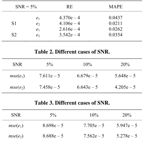
Table 1 shows the obtained results of each statistical indicator in the system (S1) and (S2) in the case of fixed learning rate.

and e 0.0471 [9].

Three cases of SNR 5,10 and 20





are taken to show the influence of disturbances modeling. The obtained results are presented in Table 2 for the first system and in table 3 for the second system.

In both Tables2 and 3, when the SNR increases the

 

i

mse e decrease, it is due under the presence of dis-turbances in the system.

[image:4.595.349.501.366.499.2] [image:4.595.97.249.366.498.2]

Table 1. Values of different statistical indicators.

SNR = 5% RE MAPE

S1

S2

e1 e2 e1 e2

4.370e – 4 4.106e – 4 2.616e – 4 3.542e – 4

[image:5.595.55.285.94.322.2]

0.0437 0.0211 0.0262 0.0354

Table 2. Different cases of SNR.

SNR 5% 10% 20%

mse(e1) 7.611e – 5 6.679e – 5 5.648e – 5

mse(e2) 7.458e – 5 6.643e – 5 4.205e – 5

Table 3. Different cases of SNR.

SNR 5% 10% 20%

mse(e1) 8.698e – 5 7.705e – 5 5.947e – 5

mse(e2) 8.688e – 5 7.562e – 5 5.278e – 5

the suitable learning rate it is necessary to carry out sev- eral tests by keeping the condition that . This research of thelearning rate can slow down the phase of training. To cure this disadvantage and in order to accel-erate the phase of training, a variable learning rate is used and a fast algorithm will be developed.



0 i 1



)

5. The Proposed Fast Algorithm

The need for using a variable learning rate is to have a fast training [8-9,15-18]. To answer this condition, the difference of the estimation error at and at

is calculated [8,9].

th

i (k 1

 

k





 







 

 

1 1

i i i i

i i

e k e k y k o k

y k o k

     

 



1

(20)

We suppose that





















1 1

and

1 1

i i

i i i

y k y k y k

o k o k o k

    

    





i

(21)

by application of [8,9]



1







i i

y k o k

   1 (22) then the Equation (20) can be





 





 

   

 

 

 

 

1 1

i i i

i

i i l

lj

T T

l il il

e k e k o k

o k

e k f h

p k

We introduce (10) and (12),





 

 

 

     

 

   

 

1

+

i i

T

l i l

T T

il i l il i

e k e k

i

f h F Pv f h F Pv e k

z F Pv f h F Pv z v e k v

 

  



 

  _



   _

(24)

so we find





 

 

   

   

 

   

2 2

1

T

i i i l

T T

il il i

i i i

e k e k f h F Pv F Pv

z F Pv F Pv z v v e k

k e k

 

 

 

    _



 

 _

 

(25)

with

 

 

  

   

2 2

_il

T

i l

T

il

k f h F Pv F P

z F Pv F Pv z v v

   _



 

 _



T

v

(26)

at



k1



the ith estimation error is



1



1

 

i i i

e k  _   k _e ki

 

(27)

To ensure the convergence of the th estimation error,

i i.e., lim i

 

0

ke k  , the condition 1 i i

 

k 1 has to

be satisfied [8,9]. This condition implies

 

1 0 i 2i k



 

i

. It is clear that the upper range of the learning rate ( ) is variable because i

 

k depends on

, il and lj. The fastest learning occurs when the

learning rate is:

v z p

 

   



   



1_{( ) 1} 2 _'2

_il ' '

T

i i l

T T

il

k f h F Pv F

z F Pv F Pv z v v

 _  _  _

 

 _

Pv

(28)

Note that this selection of i implies



1



1

   

0

e k_i   _  _{i i} k _e k_i  . It’s certain that the

learning process cannot finish instantly because of the approximation which is caused by the finite sampling time contrary to the theory which is proved that it can be happen if infinitely fast sampling can occur.

lj f h F Pv z z F Pv P v

 



    



   

 

 

  _    _

(23)

Using the obtained variable learning rate i, the syn-

certain that the learning process cannot finish instantly because of the approximation caused by the finite sam-

pling time contrary to the theorie which proved that it can be happen if infinitely fast sampling can occur.

     

   

 

   

i

   

il i l i _{T T}

l il

F Pv e k

z f h F Pv e k

T il f h F Pv F Pv z F Pv F Pv z v v  

 

  

 

 _    _ (29)

   

 

 

 

   

   

( )

il i T

lj i l il i T T

l il

F Pv z v e k

p f h F Pv z v e k

T

T il

f h F Pv F Pv z F Pv F Pv z v v

 





 

  

 

 _    _ (30)

Finally, zil

 

k and plj can be:

 





   

   

   

1

( )

i

il il T T

l il

F Pv e k

z k z k _T

il f h F Pv F Pv z F Pv F Pv z v v 

  

 

 _    _ (31)

 





 

 

 

   

   

1 il i

lj lj T T

l il

F Pv z v e k

p k p k

T

T il

f h F Pv F Pv z F Pv F Pv z v v





  

 

 _    _ (32)

rate, the neural output 1 follows the measured output 1 with an error of prediction 1 and that 2 follows the measured output 2 with an error of predict- tion 2

o

y e 0.0634 o

y 0.0588

e  . However, if b₁0 and b₂0, the error of prediction is e10.0175 and e20.0369 [9].

5.1. Simulation Results of System (S1) (SNR5)

In this section, the obtained variable learning rate (1,2) are applied. In Figure 7, the evolution of the process output and the NN output of the system (S1) is presented. The error estimation between these two outputs is pre- sented in Figure 8.

5.2. Simulation Results of System (S2) (SNR5)

The obtained results present that for a variable learning

The evolution of the process output and the NN output of the system (S2) is presented in Figure 9. The error be- tween these two outputs is presented in Figure 10. The evolution of the squared error in two cases; fixed and variable learning rates is presented in Figures 11 and 12.

0 200 400 600 800 1000 -8

-6 -4 -2 0

Pr

o

c

e

s

s

O

u

tp

u

t (

r)

: y

1

&

NN (b

)

: o

1

k

0 200 400 600 800 1000 -8

-6 -4 -2 0

P

roc

e

s

s

O

u

tput

(r

) :

y 2

&

N

N

(b

) :

o 2

k

The obtained results, concerning system (S2), present that for a variable learning rate, the neural output 1 follows the measured output with an error of pre- dicttion

o

1

y

1 0.0539

e  and that ₂ follows the measured output with an error of prediction

o

2

y e₂0.0668.

0 200 400 600 800 1000 -0.1

0 0.1

L

ear

ni

ng

E

rr

or

:

e1

k

0 200 400 600 800 1000 -0.1

0 0.1

Lear

ni

ng E

rr

or

:

e2

[image:6.595.88.249.430.686.2]

k

Figure 7. Output of process and NN of system (S1) using a variable learning rate.

[image:6.595.338.505.547.693.2]

0 200 400 600 800 1000 -8

-6 -4 -2 0

P

roc

es

s

Out

put

(r) :

y1

&

N

N

(b)

: o

1

k

0 200 400 600 800 1000 -8

-6 -4 -2 0

P

roc

es

s

Ou

tput

(r) :

y2

&

N

N

(b

) :

o2

k

Figure 9. Output of process and NN of system (S2) using a variable learning rate.

0 200 400 600 800 1000 -0.1

0 0.1

Lear

ni

n

g E

rr

or

:

e1

k

0 200 400 600 800 1000 -0.1

0 0.1

Lear

nin

g

E

rr

o

r :

e2

k

Figure 10. Learning error between the output of process and NN.

However, if and , the error of prediction

is 1and [9].

0 b 

2 2

0 b  0.0166

1 2

The obtained results presented in Figures 11 and 12 showing that, when a variable learning rate is used, the convergence of the squared error is very faster than a fixed learning rate is used.

0.029

e  e 

Table 4 shows the obtained results of each statistical indicator in the system (S1) and (S2) in the case of vari- able learning rate.

We took three cases of to show

the influence of disturbances modeling. The obtained results are presented in Table 5 for the first system and in Table 6 for the second system. In both tables, when the increases the decrease, it is due un- der the presence of disturbances in the system.

(5,10 and 20) SNR

( )i

e e

SNR ms

The obtained values in Tables 5 and 6 are lower compared to which are calculated in Ta- bles 2 and 3, that explains the variable rate adjusts with

( )i

mse e ( )i

e e ms

0 200 400 600 800 1000 0

0.5 1x 10

-8

iterations

M

e

an

S

q

u

e

r

E

rror Fixed rate:0.32

Variable rate

0 200 400 600 800 1000 0

2 4 6 8x 10

-4

iterations

M

ean S

q

u

e

r E

rror fixed rate:0.27

Variable rate

Figure 11. Evolution of the mean squared error of (S1).

0 200 400 600 800 1000 0

1 2 3x 10

-9

iterations

M

ean S

quer

E

rr

or Fixed rate:0.3 Variable rate

0 200 400 600 800 1000 0

2 4 6 8x 10

-3

iterations

me

an S

que

r

E

rr

o

r

fixed rate:0.25 Variable rate

Figure 12. Evolution of the mean squared error of (S2).

Table 4. Values of different statistical indicators.

SNR = 5% RE MAPE

S1

S2

e1 e2 e1 e2

3.256e – 4 3.793e – 4 6.453e – 4 6.236e – 4

0.0326 0.0379 0.0645 0.0624

Table 5. Different cases of SNR.

SNR 5% 10% 20%

mse(e1) mse(e2)

5.906e – 5 6.501e – 5

5.152e – 5 5.552e – 5

3.932e – 5 4.310e – 5

Table 6. Different cases of SNR.

SNR 5% 10% 20%

mse(e1)

changes in examples.

6. Conclusions

In this paper, a variable learning rate for neural modeling of multivariable nonlinear stochastic system is suggested. This parameter can slow down the training phase when it is chosen as small, and can be unstable when it is chosen as large. To avoid this step, a variable learning rate method is developed and it is applied in identification of nonlinear stochastic system. The advantages of the pro- posed algorithm are firstly the simplicity to apply it in a multi-input multi-output nonlinear system. Secondly, the gain of the training time is remarked and the result qual- ity is noticed. Besides, this algorithm is a manner to avoid the search for such fixed training rate which pre- sents a disadvantage at the level the phase of training. In contrary, the variable learning rate algorithm does not require any experimentation for the selection of an ap- propriate value of the learning rate. The proposed algo- rithm can be applied in real time process modeling. Dif- ferent cases of SNR are discussed to test the developed method and it showed that the obtained results using a variable learning rate is very satisfy than when the fixed learning rate was used.

7. References

[1] K. Kara, “Application des Réseaux de Neurones à l’identification des Systèmes Non Linéaire,” Thesis, Con- stantine University, 1995.

[2] S. R. Chu, R. Shoureshi and N. Tenorio “Neural Net-works for System Identification,” IEEE Control System Magazine, Vol. 10, No. 3, 1990, pp. 31-35.

[3] S. Chen and S. A. Billings, “Neural Networks for Non- linear System Modeling and Identification,” Inernational Journal of Control,Vol. 56, No. 2, 1992, pp. 319-346.

doi:10.1080/00207179208934317

[4] N. N. Karabutov, “Structures, Fields and Methods of Iden- tification of Nonlinear Static Systems in the Condi-tions of Uncertainty,” Intelligent Control and Automation (ICA), Vol. 1, No. 1, 2010, pp. 1-59.

[5] D. C. Psichogios and L. H. Ungar, “Direct and Indirect Model-Based Control Using Artificial Neural Networks,” Industrial and Engineering Chemistry Research, Vol. 30, No. 12, 1991, pp. 25-64.

doi:10.1021/ie00060a009

[6] A. Errachdi, I. Saad and M. Benrejeb, “On-Line Identify- cation Method Based on Dynamic Neural Network,” In-ternational Review of Automatic Control, Vol. 3, No. 5,

2010, pp. 474-479.

[7] A. M. Subramaniam, A. Manju and M. J. Nigam, “A Novel Stochastic Algorithm Using Pythagorean Means for Minimization,” Intelligent Control and Automation, Vol. 1, No. 1, 2010, pp. 82-89.

doi:10.4236/ica.2010.12009

[8] D. Sha and B. Bajic, “On-Line Adaptive Learning Rate BP Algorithm for MLP and Application to an Identifica-tion Problem,” Journal of Applied Computer Science, Vol. 7, No. 2, 1999, pp. 67-82.

[9] A. Errachdi, I. Saad and M. Benrejeb, “Neural Modelling of Multivariable Nonlinear System. Variable Learning Rate Case,”18th Mediterranean Conference on Control and Automation, Marrakech, 2010, pp. 557-562.

[10] P. Borne, M. Benrejeb and J. Haggege, “Les Réseaux de Neurones. Présentation et Application,” Editions Technip, Paris, 2007.

[11] S. Chabaa, A. Zeroual and J. Antari, “Identification and Prediction of Internet Traffic Using Artificial Neural Net- Works,” Journal of Intelligent Learning Systems & Ap- plications, Vol. 2, No. 1, 2010, pp. 147-155.

[12] M. Korenberg, S. A. Billings, Y. P. Liu and P. J. Mcllroy, “Orthogonal Parameter Estimation Algorithm for Non- linear Stochastic Systems,” International Journal of Con-trol, Vol. 48, No. 1, 1988, pp. 346-354.

doi:10.1080/00207178808906169

[13] A. Errachdi, I. Saad and M. Benrejeb, “Internal Model Control for Nonlinear Time-Varying System Using Neu-ral Networks,” 11th

International Conference on Sciences and Techniques of Automatic Control & Computer Engi-neering, Anaheim, 2010, pp. 1-13.

[14] D. Sha, “A New Neural Networks Based Adaptive Model Predictive Control for Unknown Multiple Variable No-Linear systems,” International Journal of Advanced Mechatronic Systems, Vol. 1, No. 2, 2008, pp. 146-155.

doi:10.1504/IJAMECHS.2008.022013

[15] R. P. Brent, “Fast Training Algorithms for Multilayer Neural Nets,” IEEE Transactions on Neural Networks, Vol. 2, No. 3, 1991, pp. 346-354.

doi:10.1109/72.97911

[16] R. A. Jacobs, “Increase Rates of Convergence through Learning Rate Adaptation,” IEEE Transactions onNeural Networks, Vol. 1, No. 4, 1988, pp. 295-307.

[17] D. C. Park, M. A. El-Sharkawi and R. J. Marks, “An Adaptively Trained Neural Network,” IEEE Transactions on Neural Networks, Vol. 2, No. 3, 1991, pp. 334-345.

doi:10.1109/72.97910

[18] P. Saratchandran, “Dynamic Programming Approach to Optimal Weight Selection in Multilayer Neural Net-works,” IEEE Transactions on Neural Networks, Vol. 2, No. 4, 1991, pp. 465-467. doi:10.1109/72.88167

Nomenclature

i

y

:

vector of process output, its average valuey_i,

i

u : vector of process input,

p

f : unknown function of process,

1

n : input delay,

2

n : output delay, n₁n₂,

U : input of the process, U  _u k₁

 

_u_n

 

k _T, Y: output of the process, Y  _y k₁

 

_y_ns

 

k _T,

i

o: vector of RNN output,

O: output of the RNN model, O



o₁o_ns



T,

1

N : number of nodes of input layer,

2

N : number of nodes of hidden layer,

lj

p : synaptic weights of the input layer towards the hid-den layer, P   plj with and

,

2 1, , l _ N

1 1, , j _ N

v : input vector of the RNN model,





1

1

1

2

( ) ( 1) ( ) ( 1)

N

i i i

i

v v v

u k u k n y k

y k n

 

  

  

 

  

,

ns: number of nodes of output layer,

il

z : synaptic weights of hidden layer towards the output layer, Z

 

zil with l1, , N2 and i1, , ns,

i

 : learning rate, 0i1,

: a scaling coefficient used to expand the range of RNN output, 0  1,

f : activation function, f h

 

l is the output of the

node,

th l

 

i

e k : error between the measured process output and the measured RNN output,

th i th

i

 

 

i

 

e ki yi( k o k ,

E: vector of error, E _e k₁

 

e_ns

 

k _T,

N: number of observations, TDL: Tapped Delay Line block,

l

h: th output of neuron of hidden layer, l

 

 

1

 

2

T

N

F Pv  f h _f h _

 

 

1

F Pv diag f h f

,

 

2 T

N

h

  

  _  _{ } ,

 

i

b k : noise of measurement of symmetric terminal  ,

 



,



,

b k_i    

i