Analytical and Numerical Solutions for a Rotating Annular Disk of Variable Thickness

doi:10.4236/am.2010.15057 Published Online November 2010 (http://www.SciRP.org/journal/am)

Analytical and Numerical Solutions for a Rotating Annular

Disk of Variable Thickness

Ashraf M. Zenkour1,2_{, Daoud S. Mashat}1

1_{Department of Mathematics, Faculty of Science, King AbdulAziz University,} Jeddah, Saudi Arabia

2_{Department of Mathematics, Faculty of Science, Kafrelsheikh University, Kafr El-Sheikh, Egypt} E-mail: [email protected]

Received July 19, 2010; revised October 9, 2010; accepted October 12, 2010

Abstract

In this paper, the analytical and numerical solutions for rotating variable-thickness solid disk and numerical solution for rotating variable-thickness annular disk are presented. The outer edge of the solid disk and the inner and outer edges of the annular disk are considered to have clamped boundary conditions. Two different cases for the radially varying thickness of the solid and annular disks are given. The numerical solution as well as the analytical solution is available for the first case of the solid disk while the analytical solution is not available for the second case of the annular disk. Both analytical and numerical results for displacement and stresses will be investigated for the first case of radially varying thickness. The accuracy of the present numerical solution is discussed and its ability of use for the second case of radially varying thickness is in-vestigated. Finally, the distributions of displacement and stresses will be presented and the appropriate com-parisons and discussions are made at the same angular velocity.

Keywords: Rotating, Annular Disk, Solid Disk, Finite Difference Method

1. Introduction

The problems of rotating solid and annular disks have been performed under various interesting assumptions and the topic can be easily found in most of the standard elasticity books [1-5]. Most of the research works are concentrated on the analytical solutions of rotating disks with simple cross-section geometries of uniform thick- ness and especially variable thickness [6-14]. The ana- lytical elasticity solutions of such rotating disks are avai- lable in many books of elasticity.

As many rotating components in use have complex cross-sectional geometries, they cannot be dealt with using the existing analytical methods. Numerical me- thods, such as the finite element method [15], the boundary element method [16] and Runge-Kutta’s algo- rithm [17], can be applied to cope with these rotating components.

In this paper, we will present the analytical solution for the rotating solid disk with arbitrary cross-section of continuously variable thickness. In the following, a unified governing equation will be first derived from the basic equations of the rotating disks and the proposed

stress-strain relationship. Next, finite difference method (FDM) is introduced to solve the governing equation. A comparison between both analytical and numerical solutions is made. The accuracy of the numerical solu- tion is used to find the displacement and stresses of rotating variable-thickness annular disk whose analytical solution is not available. Finally, a number of numerical examples are given to demonstrate the validity of the proposed method.

2. Basic Equations

As the effect of thickness variation of rotating disks can be taken into account in their equation of motion, the theory of the variable-thickness disks can give good results as that of the uniform-thickness disks as long as they meet the assumption of plane stress. After consi- dering this effect, the equation of motion of rotating disks with variable thickness can be written as





2 2

d

0,

stresses, r is the radial coordinate,  is the density of the rotating disk,  is the constant angular velocity, and h is the thickness which is function of the radial coordinate r.

The relations between the radial displacement ur and the strains are irrespective of the thickness of the rotating disk. They can be written as

d

, ,

d

r r

r

u u

r  r

    (2) where r and  are the radial and circumferential

strains, respectively.

For the elastic deformation, the constitutive equations for the rotating disk can be described with Hooke’s law

, .

r r

r _E    _E

   

      (3)

Using (2) into Equation (3), one can obtain the constitutive equations for _r and _ as:

2

2

d

, d

1

d . d 1

r r

r

r r

u u

E

r r

u u

E

r r



 



 



 

 _  _

  

 

 _  _

  

(4)

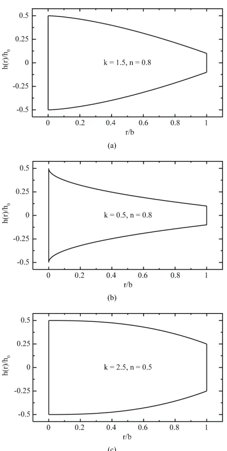
Let us consider a symmetric thin disk with respect to the mid-plane, its profile varying in the radial direction according to the formula see Figure 1:

 

0 1 ,

k

r

h r h n

b

 _{ }     _{ } 

 

 

  (5) where h0 is the thickness at the axis of the disk, n and k are geometric parameters h r( ) (0  n 1,k0), and b is the outer radius of the solid disk. A uniform-thickness disk is obtained by setting n = 0 and a linearly decreasing thickness is obtained by setting k = 1. Furthermore, if k < 1, the profile is concave and if k > 1, it is convex. The thickness of the disk is assumed to be sufficiently small compared to its diameter so that

3. Formulation and Elastic Solution for Solid

Disk

The substitution of Equations (4) and (5) into Equation (1) produces the following confluent hypergeometric differential equation for the radial displacement u rr( ) :

 

 

 

 

2 2

2

2 2 3

d d

1 (1 )

d

d ₁

1

1 0.

1

k

r r

k

k

r k

u r _r u

r n k

b r

r _n r

b r kn

b _{u r}

E r

n b 

 

 

 _   _

 



 

  

 _{ }  

 _ 

 

(6)

(a)

(b)

[image:2.595.309.541.70.531.2]

(c)

Figure 1. Variable-thickness solid disk profiles for (a) k = 1.5 and n = 0.8; (b) k = 0.5 and n = 0.8 and (c) k = 2.5 and n

= 0.5.





 

 

















2

2

2 2 2

1 ,

,

, , ,

1

, , .

r

r r

r r

R r b

b E

U R u r

b E

 

 

  

   



   



  

  

  



(7)

simple form









2 2 2 3 1 1 d d d d 1 1 1 0. 1 k k k k

n k R R

U U

R

R

R nR

n k R

U R nR                (8)

The general solution of the above equation can be written as

 

1 1

 

2 2

 

 

,

U R C F R C F R P R (9)

where C1 and C2 are arbitrary constants and F1 and 2

F are given by:

 





  



1 , , , ,

k

F R RH    nR (10)

 





 





2

1

1 , 1 , 2 , k ,

F R H nR

R   

    (11)

in which









2 2 4 1 1 1 , 2 2 4 1

1 1 _{, 1} 2_.

2 2

k k

k k

k k

k k k

                 (12)

The functions H([ , ], [ ], )   z are the generalized hyper-geometric functions,



  





   

_{ }

0 , , , , ! 0, 1,

q q q

q _q

H z z

q z            



₍₁₃₎

where ( ) q is the Pochhammer symbol given by

 

 _q  



1



 2 ...

 

 q 1







_{ }

q



,



 

     

 (14) in which  represents Gamma function.

The term P R( ) in Equation (9) is the particular solution of Equation (8) which can be written as

 



2



 

2 2

 

 

2 1

 

1 2

4 R F R d R F R d ,

P R  k _F R R F R R_

 







 (15) where



1



2



k 1 4



2



2 2 2





1



1



k 3 , nk  k R F F k F  k F nk  R F

      _    _ (16)

in which

 





 





3 1 , 1 , 1 , ,

k

F R R H    nR (17)

 





 





4 1

2 , 2 , 3 , k ,

F R H nR

R   

    (18)

The substitution of Equation (9) into Equation (4) with the aid of the dimensionless forms given in Equation (7) gives the radial and circumferential stresses in the forms of (19) and (20):

 

1 1 2 1 3 2 2







2 1 4

1 1

1 1 d

,

2 2 d

k k

r

k nR

k nR P P

R C F F C F F

R k R k R R

 

   

     _   _    _  _ 

    (19)

 

1 1 2 1 3 2 2







2 1 4

1 1

1 1 d _.

2 2 d

k

k _{k nR}

k nR P P

R C F F C F F

R k R k R R



  

  

     _   _    _  _ 

    (20)

4. Analytical Solution for the Rotating Solid

Disk

The analytical elastic solution for the solid disk with variable-thickness is completed by the application of the boundary conditions. Since the radial displacement should be vanished and the stresses should be finite at the center of the disk, then the constant C₂ vanishes. The radial displacement is vanished at the outer edge of the disk, r = b or (R = 1), hence

 

 

1 1 1 . 1 P C F

  (21)

So, one can easily obtain the solution for the present rotating variable-thickness solid disk by the substitution

of Equation (21) into Equations (9), (19) and (20).

5. Finite Difference Algorithm for Solid Disk

The resolution of the elastic problem of rotating disk with variable thickness is to solve a second-order differential equation, Equation (8), under the given boundary conditions. This equation can be written in the following general form:

 

 

 

 

 

,

0 1, 0 1 0,

U p R U q R U s R

R U U

  

    (22)

 









 









 

2 1 1 , 1 1 1 , 1 . k k k k n k R p R

nR R

n k R

q R

nR R

s R R

            (23)

It is clear that the above problem has a unique solution because ( ), ( ),p R q R and ( )s R are continuous on the given interval ]0,1] and ( ) 0q R  on ]0,1]. The linear second-order boundary value problem given in Equation (22) requires that difference-quotient approximations be used for approximating U and U. First we select an integer N0 and divided the interval ]0,1] into

(N1) equal subintervals, whose end points are the mesh points Ri  i R, for i0,1,...,N1, where

1/ ( 1)

R N

   . At the interior mesh points, ,Ri

1, 2,..., ,

i N the differential equation to the approximated is

 

_i

         

_{i i i i i} .

U R  p R U R q R U R s R (24)

If we apply the centered difference approximations of ( )i

U R and U R( )i to Equation (24), we arrive at the system:

 

 

 

   

2 1 2 1

1 2 ( )

2

1 ,

2

i i i i

i i i

R

p R U R q R U

R_{p R U R s R}

     _{ }  _{ } _   _       _{ }      (25)

for each i1, 2,..., .N The N equations, together with the boundary conditions

0 1 0, 0, N U U  

 (26)

Are sufficient to determine the unknowns Ui, 0,1, 2,..., 1

i N . The resulting system of Equations (25) is expresses in the tri-diagonal N N -matrix form:

,

AU B (27) where

   

 

 

 

 

2 , , 1 , 1 , , 2

2 , 1, 2,..., , 1 , 1, 2,..., 1,

2

1 , 2,3,..., , 2

0, 1, 2,..., 2,, 3, 4,..., , 2, , 1, 2,..., .

i i i

i i i

i i i

i j j i

i i

A R q R i N

R

A p R i N

R

A p R i N

A A i N

j N j i

B R s R i N

                          (28)

The solution of the finite difference discretization of

the two-point linear boundary value problem can therefore be found easily even for very small mesh sizes.

6. Numerical Examples and Discussion for

Solid Disk

Some numerical examples for the rotating variable- thickness solid disks will be given according the analytical and numerical solutions ( 0.3). According to Equation (7), the following dimensionless response characteristics

 

 







 

 





 

 



2

2

1 2 2

, 1 , , , . r r r E

u U R u r

b

R _ R  r _ r

             (29)

determined as per the analytical solution are compared with those obtained by the numerical FDM solution.

The results of the present investigations for the radial displacement

u

are reported in Table 1. For this example, N = 9, 19, 39 and 79, so R has the corresponding values 0.1, 0.05, 0.025 and 0.0125, respectively.

If we use the Richardson extrapolation method with 0.1,0.05,0.025,

R

  and 0.0125 we obtain results listed in Table 2. The first extrapolation is









1

4 0.05 0.1

Ext ;

3

i i

i

U  R U  R

 (30)

the second extrapolation is









2

4 0.025 0.05

Ext ;

3

i i

i

U  R U  R

 (31)

the third extrapolation is









3

4 0.0125 0.025

Ext ;

3

i i

i

U  R U  R

 (32)

the forth extrapolation is

2 1

4

16 Ext Ext

Ext ;

15

i i

i



 (33)

and the final extrapolation is

3 2

5

16 Ext Ext

Ext .

15

i i

i



 (34)

All of the results of Ext_4i and Ext_5i are correct to the decimal places listed. In fact, if sufficient digits are maintained, these approximations give results that agree with the exact solution with maximum error of

8

[image:5.595.58.288.206.686.2]

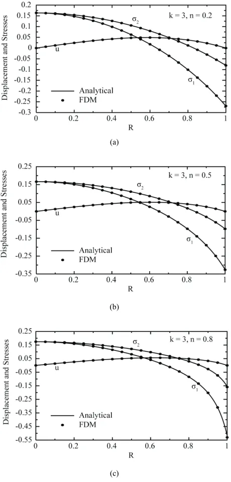
The distribution of the radial displacement, radial and circumferential stresses are presented in Figure 2. The numerical FDM solution is compared with the analytical solution for the rotating variable-thickness sold disk with k = 3 and various values of n. It is clear that, the FDM gives displacement and stresses with excellent accuracy with the exact analytical solution. It can be seen from Figure 2 that the FDM can describe the displacement and stresses through-the-thickness very well enough.

(a)

(b)

(c)

Figure 2. Dimensionless radial displacement u, radial stress

σ1 and circumferential stress σ2 for the variable-thickness solid disk (k = 3): (a) n = 0.2, (b) n = 0.5 and (c) n = 0.8.

7. Formulation and Numerical Solution for

Annular Disk

Here we consider a thin annular disk varies continuously in the form of a form of a general parabolic function (see Figure 3):

 

0 1 ,

k

r a

h r h n

b a

 _{  }      _  

 

 

  (35)

(a)

(b)

(c)

Figure 3. Variable-thickness annular disk profiles for (a) k

= 1.5 and n = 0.8, (b) k = 0.5 and n = 0.8 and (c) k = 2.5 and

where a is the inner radius of the annular disk. The equilibrium equation corresponding to Equation (35) may be easily given but its analytical solution is not.

The substitution of Equations (4) and (35) into Equa- tion (1) with the help of the dimensionless forms given in Equation (7), produces the following confluent hyper- geometric differential equation for the radial displace- ment U R( ) of the annular disk:

(a)

(b)

[image:6.595.308.539.75.272.2]

(b)

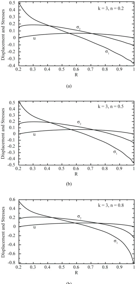
Figure 4. Dimensionless radial displacement u, radial stress

σ1 and circumferential stress σ2 for the variable-thickness annular disk (k = 3): (a) n = 0.2, (b) n = 0.5 and (c) n = 0.8.

Figure 5. Dimensionless radial displacement u of the variable-thickness annular disk for di®erent values of k

and n.

















2 2

2

4

d ₁ d

d

d 1

1 0,

1

k k

k k

U nkRR U

R R

R

R R A nR

n kRR R

U R A

R A nR



 

 

 

   

 

 

 

   



   

 

(36)

where

, .

1

a R A

A R

b A



 

 (37)

Making analogous steps as given for the solid disk, Equation (36) can be written in the following general form:

 

 

 

 

 

,

1, 1 0,

U p R U q R U s R

A R U A U

  

    (38) where the prime ( ') denotes differentiation with respect to R and

 









 









 

2 2

1 _{1 ,}

1

1

1 ,

1

.

k

k

k

k

nkRR p R

R R A nR

n kRR q R

R R A nR

R s R

R A 

 

 

  

   

 

 

 

 

   

 

  

(39)

[image:6.595.56.288.196.672.2]

and circumferential stresses. Taking n = 0.2, 0.5 and 0.8, and k = 0.5, 1.5, 2.5 and 3 in the variable thickness function given in Equation (35), a rotating annular disk with such variable thickness is studied. The inner and outer radii of the disk are taken to be a = 0.2 b (R = A = 0.2) and b (R = 1), and the results are given in terms of the rotating angular velocity. The results calculated with the FDM for displacement and stresses of a rotating variable-thickness annular disk are given in Figures 3-7.

8. Conclusions

[image:7.595.56.287.246.442.2]

This paper presents a unified numerical method for the

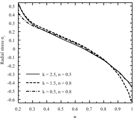
Figure 6. Dimensionless radial stress σ1 in the variable- thickness annular disk for different values of k and n.

Figure 7. Dimensionless circumferential stress σ2 in the variable-thickness annular disk for di®erent values of k

and n.

elastic calculation of rotating disks with a general, arbi- trary configuration. The governing equation was derived from the equilibrium equation and the stress- strain relationship. The analytical solution was given for the rotating variable-thickness solid disk. The calculation of the rotating sold and annular disks was turned into finding the solution of a second-order differential equa- tion under the given conditions at two boundary fixed points. Finite difference method algorithm was intro- duced to solve the governing equation for both solid and annular disks and a number of numerical examples were studied. The results from the analytical and FDM solutions were compared. The proposed FDM approach gives very agreeable results to the analytical solution.

9. Acknowledgements

The investigators would like to express their appreciation to the Deanship of Scientific Research at King AbdulAziz University for its financial support of this study, Grant No. ع/168/428.

10. References

[1] S. P. Timoshenko and J. N. Goodier, “Theory of Elastic-ity,” McGraw-Hill, New York, 1970.

[2] S. C. Ugral and S. K. Fenster, “Advanced Strength and Applied Elasticity,” Elsevier, New York, 1987.

[3] U. Gamer, “Tresca’s Yield Condition and the Rotating Disk,” ASME Journal of Applied Mechanics, Vol. 50, No. 2, 1983, pp. 676-678.

[4] U. Gamer, “Elastic-Plastic Deformation of the Rotating Solid Disk,” Ingenieur-Archiv, Vol. 45, No. 4, 1984, pp. 345-354.

[5] A. M. Zenkour, “Analytical Solutions for Rotating Ex-ponentially-Graded Annular Disks with Various Bound-ary Conditions,” International Journal of Structural Sta-bility and Dynamics, Vol. 5, No. 4, 2005, pp. 557-577. [6] U. Güven, “Elastic-Plastic Stresses in a Rotating Annular

Disk of Variable Thickness and Variable Density,” In-ternational Journal of Mechanical Sciences, Vol. 34, No. 2, 1992, pp. 133-138.

[7] U. Güven, “On the Stress in the Elastic-Plastic Annular Disk of Variable Thickness under External Pressure,” In-ternational Journal of Solidsand Structures, Vol. 30, No. 5, 1993, pp. 651-658.

[8] U. Güven, “Stress Distribution in a Linear Hardening Annular Disk of Variable Thickness Subjected to Exter-nal Pressure,” International Journal of Mechanical Sci-ences, Vol. 40, No. 6, 1998, pp. 589-601.

[image:7.595.57.286.477.678.2]

[10] A. N. Eraslan, “Inelastic Deformation of Rotating Vari-able Thickness Solid Disks by Tresca and Von Mises Cri-teria,” International Journal for Computational Me- thods in Engineering Science, Vol. 3, 2000, pp. 89-101. [11] A. N. Eraslan and Y. Orcan, “On the Rotating

Elas-tic-Plastic Solid Disks of Variable Thickness Having Concave Profiles,” International Journal of Mechanical Sciences, Vol. 44, No. 7, 2002, pp. 1445-1466.

[12] A. N. Eraslan, “Stress Distributions in Elastic-Plastic Rotating Disks with Elliptical Thickness Profiles Using Tresca and von Mises Criteria,” Zurich Alternative Asset Management, Vol. 85, 2005, pp. 252-266.

[13] A. M. Zenkour and M. N. M. Allam, “On the Rotating Fiber-Reinforced Viscoelastic Composite Solid and An-nular Disks of Variable Thickness,” International Journal

for Computational Methods in Engineering Science and Mechanics,Vol.7, No. 1, 2006, pp. 21-31.

[14] A. M. Zenkour, “Thermoelastic Solutions for Annular Disks with Arbitrary Variable Thickness,” Structural Engineering and Mechanics, Vol. 24, No. 5, 2006, pp. 515-528. [15] O. C. Zienkiewicz, “The Finite Element Method in

Engi-neering Science,” McGraw-Hill, London, 1971.

[16] P. K. Banerjee and R. Butterfield, “Boundary Element Methods in Engineering Science,” McGraw-Hill, New York, 1981.