Algorithms for Tissue Image Analysis using Multifractal Techniques

(1)

Algorithms for

Tissue Image Analysis using

Multifractal Techniques

A thesis submitted in partial fulfilment

of the requirements for

the Degree of Master of Science

in Computer Science and Software Engineering

in the University of Canterbury

by

ChiangHau TAY

Dr R. Mukundan……….. Supervisor Associate Professor, Department of Computer Science and Software Engineering

Dr D. Racoceanu……….Co-Supervisor Director, Image & Pervasive Access Lab, Singapore

University of Canterbury

(2)

Abstract

Histopathological classification and grading of biopsy specimens play an

important role in early cancer detection and prognosis. Nottingham Grading System

(NGS) is one of the standard grading procedures used in breast cancer assessment,

where three parameters, Mitotic Count (MC), Nuclear Pleomorphism (NP), and

Tubule Formation (TF) are used for prognostic information. The grading takes into

account the deviations in cellular structures and appearance between tumour and

normal cells, using measures such as density, size, colour, and regularity. Cell

structures in tissue images are also known to exhibit multifractal characteristics.

This research focused on the multifractal properties of several graded biopsy

specimens and analysed the dependency and variation of the fractal parameters

with respect to the scores pre-assigned by pathologists. The effectiveness of using

multifractal techniques on breast cancer grading was measured with a set of

quantitative evaluations for MC, NP, and TF criteria. The developed method for

MC scoring has obtained 82.87% true positive rate on detecting mitotic cells.

Furthermore, the overall positive classification rates for NP and TF analysis were

67.38% and 71.82%, respectively, while obtaining 30.26% of false classification

rate for NP analysis and 27.17% for TF analysis. The results have shown that

multifractal formalism is a feasible and novel method that could be used for

(3)

Acknowledgements

It is my pleasure to thank my supervisor Dr R. Mukundan for his guidance

and help during my research. My Masters degree could not be achieved without his

support and advice.

Special thanks to the staff members of the Image & Pervasive Access Lab

(IPAL), Singapore. This thesis would not have been possible without the support

from the director of IPAL, Dr D. Racoceanu, my co-supervisor, who has provided

valuable inputs. The group has provided essential software, histopathological

images, and related information which were extremely useful for this research. I am

grateful for the help and support received from Dr L. Roux and Dr N. Lomenie

during my visit to IPAL.

It is an honour for me to have the financial support from the Department of

Computer Science and Software Engineering for me to visit IPAL in Singapore. I

would also like to thank the Department for providing all the support and resources

required for my research.

Finally, I must acknowledge the support from my family, friends, Mrs S. Day

from Learning Skills Centre, and colleagues from the department for helping and

(4)

i

List of Figures

Figure 1-1 The top nine most frequent cancers for women worldwide, 2008 [2] .. 2

Figure 1-2 A whole slide image at a ×1.0 magnification scale [10] ... 3

Figure 2-1 The number of mitotic count per 10 HPF by the field diameter [22] ... 8

Figure 2-2 Four stages of mitosis: (a) prophase (b) metaphase (c) anaphase (d) telophase [22] ... 8

Figure 2-3 Impact of number of critical cell nuclei to the error rate of NP scoring [33]... 12

Figure 2-4 Example of (a) a histopathological image (b) results where red represents type 3 malignant, magenta represents type 2 malignant, blue represents type 1 malignant, and green represents benign object [34]... 13

Figure 2-5 Scatter plot for the classification of section images using the number of cancer cells and tubules as features parameters; C1, C2, and C3 are the quadratic classifier which associated with G I, G II, and G III (Score 1, 2, and 3) [36] ... 14

Figure 2-6 General schematic of Nottingham Grading System ... 16

Figure 3-1 Window size of w = 1, 3, 5 at the black centre pixel, p (reproduced from [40]) ... 20

Figure 3-2 The (a) original image (b) border for calculating multifractal measure ... 21

Figure 3-3 The greyscale image (left) and its corresponding intensity histogram (right) ... 23

Figure 3-4 The α-image (left) and its corresponding α-histogram (right) ... 24

Figure 3-5 The binary images produced by thresholding the α-image at different α-series ... 25

Figure 3-6 Multifractal spectrum: (a) actual form (b) continuous form ... 26

Figure 3-7 Box-counting method that uses different box sizes ε ... 27

Figure 3-8 Multifractal spectrum: (a) original discrete function (b) sixth order polynomial equation ... 29

Figure 3-9 The magnified portion of the α-histogram of the sum measure from Figure 3-4 ... 30

(7)

iv

Figure 3-11 Example of an medical image (a) original; result after: (b) Sobel operator (c) Robbers operator (d) Prewitt operator (e) Log operator (f) Hölder exponent [53] ... 31

Figure 3-12 Image of a retinal vessel structure: (a) normal (b) pathological state [58]... 32

Figure 3-13 Summary of calculating the Hölder exponent and multifractal dimension... 34

Figure 4-1 System overview of the multifractal analysis of the tissue images .... 36

Figure 4-2 Screenshots of the FrameWork Viewer ... 38

Figure 4-3 Sample images of pre-labelled: (a) NP (b) TF scores, (from top to bottom) Score 1, Score 2, and Score 3 ... 39

Figure 4-4 The developed GUI for cropping 10 sub-image frames from a NP/TF-labelled region ... 40

Figure 4-5 Tissue micro-textures identified using image processing [36] ... 41

Figure 4-6 The tissue image example of (a) epithelial type (b) non-epithelial type ... 41

Figure 4-7 The α-range of sub-image frames from a histopathological sample .. 43

Figure 4-8 The process of detecting a mitotic cell: (a) original image with a manually detected mitotic cell (b) the binary threshold image (c) the computationally detected mitotic cell ... 44

Figure 4-9 (a) The original sub-image frame, and the binary α-image of the specific α-sub-range for NP analysis: (b) max measure (c) inv-min measure (d) sum measure (e) Iso measure ... 46

Figure 4-10 (a) The original sub-image frame, and the binary α-image of the specific α-sub-range for TF analysis: (b) max measure (c) inv-min measure (d) sum measure (e) Iso measure ... 47

Figure 4-11 Multifractal spectrum for NP and TF analysis: (a) max measure (b) inv-min measure (c) sum measure (d) Iso measure ... 48

Figure 4-12 Improvement of NP analysis: (a) the original image (b) before enhancement (c) after enhancement of inv-min measure (d) before enhancement (e) after enhancement of sum measure ... 50

Figure 4-13 Improvement of TF analysis: (a) the original image (b) before enhancement (c) after enhancement of inv-min measure (d) before enhancement (e) after enhancement of sum measure ... 51

(8)

v

Figure 4-15 The features of multifractal spectrum for NP analysis: (a) max

measure (b) inv-min measure (c) sum measure (d) Iso measure ... 52

Figure 4-16 The features of multifractal spectrum for TF analysis: (a) max measure (b) inv-min measure (c) sum measure (d) Iso measure ... 53

Figure 4-17 The multifractal spectrum that uses different α-range ... 54

Figure 4-18 Multifractal spectrum of the original function and the cubic polynomial function ... 54

Figure 4-19 Displaying different colour models of an input image ... 55

Figure 4-20 Displaying multifractal spectra of four sub-image frames ... 56

Figure 4-21 Advanced application of visualization for multifractal spectrum ... 57

Figure 4-22 Displaying mitotic cell detection ... 58

Figure 4-23 Summary of pre-processing the tissue images with multifractal techniques ... 60

Figure 4-24 Summary of the procedure of breast cancer grading system ... 61

Figure 5-1 Examples of an image frame and its presentation in different colour models ... 64

Figure 5-2 The effect of different colour models to the average α-range of sum measure (×20.0) ... 65

Figure 5-3 The effect of using red channel, green channel, and greyscale to the average α-range of sum measure (×40.0) ... 66

Figure 5-4 ROI: (a) original image sample (b-c) result from Huang et al. [20, 64] (d-f) results obtained from this research: max, sum, Iso measures .... 68

Figure 5-5 The effect of α-threshold on mitotic cell detection ... 70

Figure 5-6 The effect of different α-thresholds to the average size of the mitotic cells ... 71

Figure 5-7 An unexpected behaviour of the system: (a) manually identified mitotic cell, M1 (b) a mistakenly detected mitotic cell, C1 ... 72

Figure 5-8 An undesired behaviour of the system: (a) two manually identified mitotic cells, M1 and M2 (b) a detected mitotic cell, C1, the other mitotic cells are omitted ... 73

Figure 5-9 The ROC curves for NP classification ... 77

Figure 5-10 The ROC curves for NP classification after introducing the weight factors ... 79

Figure 5-11 Two examples of α-sub-range with undeterminable local maxima .... 80

(9)

vi

List of Tables

Table 2-1 Nottingham Grading System [16]... 6

Table 2-2 NGS for Nuclear Pleomorphism [16] ... 10

Table 2-3 NGS for Tubule Formation [16] ... 14

Table 2-4 Summary of the evaluations for NGS parameters ... 17

Table 4-1 The number of image frames used for data analysis ... 40

Table 4-2 Examples of α-range from a histopathological example ... 42

Table 4-3 Properties of the multifractal spectrum for NP and TF analysis ... 48

Table 5-1 The α-threshold list for classifying the types of tissue structures ... 67

Table 5-2 The classification results for NP scores using different multifractal measures ... 76

Table 5-3 The classification results for NP scores based on the voting system of any two multifractal results ... 78

Table 5-4 The classification results for NP scores based on the combination of any two multifractal results after introducing the weight factors ... 80

Table 5-5 The classification results for TF scores using different multifractal measures ... 82

Table 5-6 The classification results for TF scores based on the combination of any two multifractal results after introducing the weight factors ... 83

(10)

vii

List of Abbreviations

ACM Active Contour Model

ASL Arterial spin labelling

ASR Age-standardised rate

AT Area that represents water, carbohydrate, lipid or gas

CMY Cyan, magenta, and yellow (colour space)

CPU Central processing unit

CT Computed tomography

ECM Collagen-based matrix

EEG Electroencephalogram

FMRI Functional Magnetic Resonance Imaging

GPU Graphics processing unit

HPF High-power field

IARC International Agency for Research on Cancer

IPAL Image & Pervasive Access Lab

MC Mitotic Count

MF-DFA Multifractal Detruded Fluctuation Analysis

NGS Nottingham Grading System

NM1 Nuclei of inflammatory cells

NM2 Cell nuclei of epithelial origin

NM3 Nuclei of cancer cells

NP Nuclear Pleomorphism

(11)

viii ROC Receiver operating characteristic

ROI Region of interest

SBR Scarff-Bloom-Richardson

SVM Support Vector Machine

SWS Slow wave sleep

TF Tubule Formation

(12)

1

Chapter 1:

Introduction

Cancer is a term that describes the uncontrolled growth of abnormal cells in

the body [1]. Normal cells follow the orderly path of growth, division, and death.

Cancer cells begin to form when this process breaks down, as they continue to

expand and divide. This leads to a mass of abnormal cells that grows out of control.

Healthy tissue can be invaded by cancer cells; it can harm the body when the

abnormal cells start to form lumps or masses of tissue, known as tumours, which

can interfere with the body’s system and function.

More than 100 different types of cancer have now been discovered.

According to the statistics collected by the International Agency for Research on

Cancer (IARC), breast cancer is the most frequent type of cancer among women

worldwide, as shown in Figure 1-1 [2-4]. The statistic has shown that the incidence

and mortality rates for breast cancer have rapid growth in many Eastern European,

Asian, Latin American, and African countries [5]. In addition, breast cancer is the

major cause of death for women in several developing and developed countries.

Lack of funding and resources are the reason why these patients do not receive

(13)

[image:13.595.126.465.111.333.2]

2

Figure 1-1 The top nine most frequent cancers for women worldwide, 2008 [2]

Studies have shown that death from breast cancer can be reduced if the

disease is managed. An age-standardised rate (ASR) was introduced to adjust the

population age structures based on different periods of time, geographic areas, and

population sub-groups. ASR is the ratio of a specific rate in the population being

studied over the population of an age group in standard population [6]. A health

services research showed the incidence rate of breast cancer is 39.0 ASR per

100,000 people, while the mortality rate is 12.5 ASR per 100,000 people.

Compared to lung cancer which has a high incidence-to-mortality ratio of 1: 0.81,

breast cancer has a lower ratio of 1: 0.32 [2]. Improving disease management can

increase the chances of survival and recovery from breast cancer [7].

1.1 Motivation

Early detection plays an important role in reducing cancer mortality. The

current procedure for breast cancer grading is manually performed by pathologists.

Breast tissue samples of patients are taken and examined under microscopes.

Pathologists grade the tissue samples based on the deviation of the cell structures

from normal tissues. A pathologist may have to examine hundreds of slides daily

[8], which is a subjective and time consuming process.

0 10 20 30 40

Breast

Colorectum

Cervix uteri

Lung

Stomach

Corpus uteri

Liver

Ovary

Thyroid

ASR rate per 100,000

Incidence

(14)

3

Histopathological images (images of biopsy samples) are now available in

high resolution and high magnification digital format which can be further

processed to extract useful structural information. However, the manual analysis of

such huge sets of data can be time consuming [9]. Figure 1-2 is an example of a

compressed image of a full size histopathological image. The original size of this

biopsy sample was 14,654 μm × 11,026 μm. At a ×40.0 magnification scale, this

histopathological image can be represented in digital format with a resolution of

[image:14.595.99.500.276.585.2]

58,630 × 44,216 pixels, and it requires 449,149 Kb of digital data storage.

Figure 1-2 A whole slide image at a ×1.0 magnification scale [10]

The medical data used in this research were provided by Image & Pervasive

Access Lab (IPAL), Singapore. The research group in IPAL is constructing a

“cognitive virtual microscopic framework” for the breast cancer grading system.

This framework introduces a “knowledge-driven medical imaging environment”; it

can provide a system that is effective, efficient, reliable, and traceable assistance

(15)

4

George and Sager showed that tumours can be classified using the

multifractal techniques [11]. This research is going beyond George and Sager’s

research to measure the effectiveness of using multifractal techniques to grade the

tissues of breast cancer tumours.

1.2 Objectives

Cell structures have multifractal characteristics that could be directly used for

identifying pathological conditions. Multifractal formalism has been developed by

many researchers; it has been recently used in the domain of biomedical image

processing. Applying multifractal techniques is a novel approach for analysing

breast cancer grading. This research aims to explore the relationship between

various multifractal measures of cell structures in the tissue samples and the

corresponding scores assigned by pathologists.

However, this grading system does not replace the work of pathologists;

rather, it provides a pre-screening analysis for them. The system should reduce the

workload of pathologists and alert them to the cases that require closer attention.

1.3 Publication

The work of this Master’s research has been published in the 26th

International Conference Image and Vision Computing New Zealand

(IVCNZ 2011). The details of the paper are as follows:

ChiangHau Tay, Ramakrishnan Mukundan, and Daniel Racoceanu.

Multifractal Analysis of Histopathological Tissue Images. In Image and

Vision Computing New Zealand. IVCNZ ’2011. 26th International

(16)

5

1.4 Thesis Overview

The thesis contains six chapters, and it is presented as follows:

 Chapter 2 outlines the overview of breast cancer grading and summarises the related work developed by other researches in breast cancer analysis.

 Chapter 3 contains the working procedure of multifractal technique and demonstrates the algorithms to calculate the multifractal spectrum. Several

applications of multifractal analysis are reviewed in this chapter.

 Chapter 4 presents the outline of the system structure and implementation of this research. The developed methods are fully described and explained.

 Chapter 5 contains the results and the discussion of the implemented methods.

(17)

6

Chapter 2:

Background and Literature Survey

The overview of breast cancer diagnosis is presented in this chapter. The

methods for evaluating the features of breast cancer grading are summarised.

2.1 Overview of Breast Cancer Grading

Scarff-Bloom-Richardson (SBR) system has been commonly used in the

United States since 1957 [12]. Nuclear grading was one of the main focuses in SBR

system; however, the effects of tubules have not been considered. In 1998, two

European histopathologists, Professor Elston (Professor of Tumour Pathology) and

Dr Ellis (Reader of Pathology) modified SBR system into Nottingham Grading

System (NGS) [13, 14], which focuses on three criteria: Mitotic Count (MC),

Nuclear Pleomorphism (NP), and Tubule Formation (TF). Each criterion

contributes 1 to 3 points, and they are added to give a final equivalent grade, as

shown in Table 2-1. Both Collage of American Pathologists and World Health

Organization recommended NGS for breast cancer grading [15] because NGS

introduces more specific criteria [13]. Hence it has become the current standard.

Table 2-1 Nottingham Grading System [16]

Overall grade Equivalent grade Combined histological grade

Low Grade I 3-5 points

Intermediate Grade II 6-7 points

(18)

7

However, the presence of solely a good grading system does not guarantee

the reliability of pathology results. Pathologists could analyse these medical tests

based on their experience and subjective opinions [17]; hence the grade of a cancer

case could have a low agreement between pathologists [18]. Dunne and Going

carried out a case study to analyse the breast cancer grading ranked by different

pathologists. The results showed that differences might arise from individual

decision on nuclear grading in breast carcinoma. Professional pathologists

specialised in breast cancer tended to grade higher pleomorphism scores than

non-specialists [19]. Huang et al. also noticed that different doctors could give

different diagnosis for the same biopsy samples. Although it is not a usual case, a

doctor can make different prognosis on a same medical test at different times [20].

Therefore, a computer-aided system is required to provide a standard and

quantitative measurement for breast cancer assessment. Currently, many computer

science researchers focus their studies on the algorithms for automatic and

semi-automatic breast cancer grading system based on the NGS criteria. These

researches aim to perform the time-consuming pre-screening job, and to provide

(19)

8

2.2 Mitotic Count Scoring

The scoring for Mitotic Count (MC) calculates the number of mitotic cells

found in a high-power field (HPF). HPF is a term used in microscope; it refers to

the visible area under maximum magnification power of a microscope. The

diameter of the “field of view” varies between microscopes [21]; the numbers of

mitotic count related to NGS in 10 HPF is shown in Figure 2-1.

Figure 2-1 The number of mitotic count per 10 HPF by the field diameter [22]

Mitosis detection is challenging because the mitotic cells are small and have

different shapes. The mitosis has four main stages determined by the shapes of the

nucleus (Figure 2-2): prophase, metaphase, anaphase, and telophase [22, 23]. A

mitotic cell refers to the daughter cells form at metaphase, anaphase, and telophase;

whereas cells at prophase are not considered as mitotic cells [22]. Different

circumstances make the process of detecting mitotic cells even more challenging.

(a) (b) (c) (d)

(20)

9

Kamen et al. studied an automated recognition of mitosis in tissue sections in

1984. The aim of their study was to maximise the number of detected mitotic cells.

Potential mitotic cells were selected by using global and local segmentation

techniques. The global threshold separated darker elements (mitotic cells, artefacts,

and inflammatory cells) from the background pixels which were brighter; the local

threshold then performed a second sieving process to the darker elements. Contour

features were applied on classification of mitotic cells and non-mitotic cells. This

method had a result of a large net loss of 37% mitotic cells, and 5% of non-mitotic

cells were mistaken as mitotic cells [24]. Low image quality and unsuitable staining

preparation were the cause of the unsatisfactory result [25].

In 1993, Kate et al. used region growing method to segment mitotic cells [25].

The method was able to correctly classify 81% of the mitotic cells, while obtaining

30% of false positive rate. A mitotic cell has the darkest pixel in the cell region; a

seed can start from the darkest pixel and expand to the neighbouring pixels which

have similar intensity properties. During the classification process, Kate et al.

analysed contour features for detecting the hairy feature of mitotic cells and

“optical density measurements” to observe the object feature of mitosis. During the

training stage, the semi-automated method required the users’ input to classify

mitotic cells and non-mitotic cells. The system then learned from the first training

experiment and re-evaluated the entire training set. The result of the fully automatic

method was not ready for clinical practice, but the semi-automated method could

be used as a pre-screening device.

The improvement work from Kate et al. was carried on by Beliën et al. in

1997. They investigated the effects of spatial resolution on the results of automatic

mitosis recognition. The process was slow due to hardware limitation back then.

They suggested that higher resolution in breast cancer sections can improve the

resolution of the hairy features of mitotic cells, but the irrelevant artefacts formed

during the preparation of the microscope slides also gained better resolution. The

(21)

10

worked better at higher spatial resolution. They managed to reduce the false

negative rate from 19% [25] to 5-8%, but the false positive rate was still

unsatisfactory, ranging from 22% and 42% [26].

In 2008, Dalle et al. classified potential mitotic cells by matching the shapes

and intensity properties of test cells with those of mitotic cells. They captured a set

of histological image frames, each of 1,024 × 1,280 pixels, from a patient’s sample.

The average count of mitotic cells over all image frames was calculated and

multiplied by a factor of 10. NGS states that the MC score is evaluated by the total

mitotic cells found from 10 randomly selected cell regions; hence the multiplication

factor was introduced. This method was tested and compared with the results

analysed by a pathologist. Four out of six grading results agreed with the expert,

one was overestimated, and one was underestimated [27].

Segmentation of mitotic cells is complicated; researchers found that mitotic

cells are small and can be easily confused with artefacts. However, mitotic cells

have unique hairy features which make them detectable.

2.3 Nuclear Pleomorphism Scoring

Nuclear Pleomorphism (NP) score focuses on the shapes, chromatin

distribution, and sizes of cell nuclei. The score of NP is listed in Table 2-2; one of

the key factors in NP scoring is cell nuclei detection. Many methods have been

proposed for cell nuclei segmentation, such as thresholding [28], watershed [29],

morphological operation [30], and generic features [31]. However, only the

methods developed for breast cancer are reviewed in this section.

Table 2-2 NGS for Nuclear Pleomorphism [16] Score Nuclear Pleomorphism scoring

1 Small regular uniform cells

(22)

11

Cosatto et al. described a robust method for measuring the size of neoplastic

nuclei. They used an Active Contour Model (ACM) to segment cell nuclei and

classified them with a Support Vector Machine (SVM). To remove colour

variations, Cosatto et al. converted a colour image into CMY (cyan, magenta, and

yellow) colour space. Then, a 2D Difference of Gaussian filter was applied to find

the malignant cells, which are always larger than a normal nucleus. Elliptical

nuclei, which have symmetric shapes, could be detected with a Hough transform

operation. The outline of an elliptical nucleus could be approximated with ACM.

The SVM classifier was trained to analyse the shape, texture, and fitness of the

outline of the malignancies. Cosatto et al. showed that their result obtained 92%

true positive and 20% false negative in classifying malignant and benign cells [32].

Although their method had yet to provide actual NP grading, accurately measuring

the sizes of malignant cells is a key parameter in NP scoring.

Dalle et al. applied Gaussian function to model the probability distributions

of the colours of cells used for NP scoring. Each NP score had a global Gaussian

model which defined the mean and covariance matrix of the colours in its

corresponding type of cells; these models represented three types of chromatin

distribution: homogeneous, moderate, and clumped. On the other hand, every

detected cell had its own Gaussian model which was then compared with the global

model. A cell was denoted as a particular type of cell when its colour distribution

was similar to that global model. Six medical samples were tested, where three of

them were Score 2 and three were Score 3. This method had correctly classified all

medical tests with Score 2 and only one for Score 3. The other two Score 3 cases

were underestimated to be Score 2. Dalle et al. were confident to their result

because a pathologist only needs enough numbers of cell regions which are Score 2

and Score 3 to make an assessment [27].

Unlike other existing methods that tended to detect every cell in the image,

Dalle et al. showed that NP scoring could be achieved by analysing the critical cell

(23)

12

together and have larger shape than inflammatory cells and mitotic cells.

Dalle et al. first detected a region of interest (ROI), described in [27], and applied a

gamma correction to the red channel of the ROI. Gamma correction can change the

brightness and the ratio of red, green, and blue of an image; it highlighted the cell

nuclei from the background. Then, a threshold operation was applied to separate

cell nuclei and background. Nearby clusters could be connected with a dilation

operation, while the isolated clusters remained isolated. After that, an erosion

operation was applied to separate connected clusters. A candidate critical cell

nucleus was large and had close-by critical cell nuclei. The measurement for NP

score was based on the size, shape and, texture of the critical cell nuclei.

Overall, Dalle et al. found that 7.84% of cell nuclei were incorrectly

classified. Besides, they also found that the number of critical cell nuclei was

crucial for classification (Figure 2-3). To minimise the error rate to 7.8%, at least

40 cell nuclei were required for Score 3. Similarly, NP Score 2 required a minimum

of 50 cell nuclei to keep the error rate below 12%. This method used less

processing time while maintaining a good accuracy of the classification [33].

Figure 2-3 Impact of number of critical cell nuclei to the error rate of NP scoring [33]

A breast cancer detection method which combined neural network as a

classifier tool was presented by Singh et al. They classified malignant breast tumor

into three types: Type 1, Type 2, and Type 3. The adaptive thresholding method

(24)

13

separate stained tissue and background, Singh et al. assumed that local variations

occurred during the preparation did not affect the measurements. Once the

individual cells had been detected and segmented, the neural network classified

malignant and benign nuclei based on eight different nucleus characteristics. The

result of a histopathological image after applying the method is shown in

Figure 2-4. The proposed system gave an overall accuracy of 95.80%, which is

relatively high for breast tumour screening [34].

(a) (b)

Figure 2-4 Example of (a) a histopathological image (b) results where red represents type 3 malignant, magenta represents type 2 malignant, blue represents type 1 malignant, and

green represents benign object [34]

The score of NP is based on the deviation of cell nuclei in an invasive breast

tissue region. Although there are many different methods developed for cell nuclei

segmentation, literatures agreed that the performance of NP scoring is dependent

on accurate segmentation of cell nuclei.

2.4 Tubule Formation Scoring

Tubules refer to the white blobs (lumina) surrounded by a continuous string

of cell nuclei [35]. The scoring of Tubule Formation (TF) measures the percentage

of tubules present in a histopathological image. NGS for TF score is shown in

(25)

14

Table 2-3 NGS for Tubule Formation [16] Score Tubule Formation scoring

1 Majority of tubule (> 75%) 2 Moderate degree of tubule (10-75%) 3 Marked nuclear variation (< 10%)

Petushi et al. showed that the microstructure existed in a histological image

could be modelled; this model could localize TF via segmentation and machine

learning classification of the cell nuclei [36, 37]. The grading for each section

image could be distinguished by measuring the average distances between the

centroids of closest nuclei in a high density region. Besides, Petushi et al. also

noticed that there was a correlation between tubules and cancer cells. As shown in

Figure 2-5, a section image which had majority nuclei of cancer cells contained a

fewer number of tubules. Based on these texture features, the section image could

be classified as Score 1 and Score 3. The overall results had shown that this method

worked well in Score 1 and 3 cases, but the result of Score 2 was less satisfactory

[36].

Figure 2-5 Scatter plot for the classification of section images using the number of cancer cells and tubules as features parameters; C1, C2, and C3 are the quadratic classifier which

(26)

15

A “rules-based system modelling” that transformed medical concepts into

computer vision concepts were developed by Tutac et al. Their model was

developed for a full NGS diagnosis tool, but only the development for TF is

described in this section. Tutac et al. defined “DarkCellsCluster” as a symbolic rule

which contained a group of adjacent cells with intensity value setup between very

dark and white limits. The pathological criterion TF could be satisfied when the

symbolic rule for TF “WhiteBlobs” were included in the “DarkCellsCluster”. The

local grading TF (single criterion of NGS) was calculated with the ratio of TF ROI

over the area of “DarkCellsCluster”. Among six breast cancer tests which

composed to 5,600 frames, this method obtained 11% testing errors for TF scores.

Although the average single component error (including MC and NP) was 11%, the

global grading errors of NGS was 0% [35]. As a result, the final NGS grade was

not affected by single component errors.

Dalle et al. used a morphological operation to segment tubules in a low

resolution global image. A blob structure containing fat or lumina region was

considered a TF. Subsequently, the blob structures presented in the neoplasm could

be found with the morphological filling operation. The ratio of the section occupied

by tubules and the total area of cells in the image frames denoted the TF score.

However, the results based on this method tended to score lower than the

pathologist’s. Dalle et al. explained that their system had slightly stricter

measurements [27].

All researchers agreed that localising the white blobs surrounded by cell

nuclei was the first step to analyse TF score in the biopsy slides. Hence, it was an

(27)

16

2.5 Summary of Literature Review

NGS is the benchmark for breast cancer analysis, where MC, NP, and TF are

used for prognostic information, as shown in Figure 2-6. Automatic and

semi-automatic methods for breast cancer diagnosis have been developed by many

researchers. Most of the methods were proposed to address a single NGS criterion.

Only a few researches focused on complete breast cancer diagnosis tools which had

an equivalent grading result with NGS. A brief description of how literatures

approached NGS parameters is summarised in Table 2-4.

Figure 2-6 General schematic of Nottingham Grading System Nottingham

Grading System (NGS)

Mitotic Count (MC)

Score: 1, 2, 3

Nuclear Pleomorphism (NP)

Score: 1, 2, 3

Tubule Formation (TF)

Score: 1, 2, 3

Grade I ···Score 3-5 Grade II ···Score 6-7 Grade III ···Score 8-9

(28)

[image:28.595.92.506.161.433.2]

17

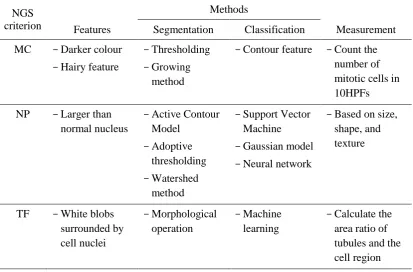
Table 2-4 Summary of the evaluations for NGS parameters

NGS criterion

Methods

Features Segmentation Classification Measurement MC -Darker colour

-Hairy feature

-Thresholding -Growing

method

-Contour feature -Count the number of mitotic cells in 10HPFs NP -Larger than

normal nucleus

-Active Contour Model

-Adoptive thresholding -Watershed

method

-Support Vector Machine -Gaussian model -Neural network

-Based on size, shape, and texture

TF -White blobs surrounded by cell nuclei

-Morphological operation

-Machine learning

(29)

18

Chapter 3:

Multifractal Analysis

Biomedical image processing involves segmentation, automatic recognition,

and classification of the image features. Image analysis for tissue and cell images is

complicated and challenging. The shapes of the tissues and cells are irregular; they

are different in size and have different orientations. Hence, performing such

complex tasks requires more advanced techniques than traditional image analysis

methods [38].

Natural objects exhibit statistical self-similarity, a repetition of form over a

variety of scales [39]. Tissues and cells have the feature of self-similarity with

varying degrees of randomness, so they belong to a class of objects known as

multifractal [40]. Multifractal refers to configurations with different observed

degree of fractal dimension, an attribute that describes the level of self-similarity

[41]. Many researchers conclude that multifractal technique is an effective and

robust tool for image segmentation and interpretation [38, 42-44]. Therefore,

multifractal technique has been widely applied in biomedical image processing.

This chapter includes the process of calculating Hölder exponent, denoted as

α-value, the description of variation in local density of the image. Moreover, the

types of multifractal measures are illustrated in detail with the properties of each

measure. The computation of multifractal spectrum, which describes the fractal

(30)

19

multifractal techniques on biomedical image processing are reviewed in Section 3.5

of this chapter.

3.1 Hölder exponent

A digital image is numerically represented by a two-dimensional array with a

configuration of M rows and N columns; each index, known as pixel, contains a

unique property. Depending on the types of digital image, the unique property of a

pixel can be different. For example, the pixels of a binary image have binary

values, the pixels of a greyscale image have intensity values, and the pixels of a

colour image have red, green, blue, and alpha values.

Multifractal describes the fractal properties of an image using an

intensity-based measure within the neighbourhood of each pixel. In an example of a

greyscale image, each pixel in the image has an intensity value which is

represented as a multi-level of grey value. These grey values are linearly

interpolated from black to white, ranging from 0 to 1. The local singularity

coefficient, also known as the Hölder exponent [38, 44, 45], or α-value, reflects the

local behaviour of a function μp(w), described in Equation 3.1, around the pixel

[46]. The window of size w, is centred at the pixel p, as shown in Figure 3-1. The

variation of the intensity measure with respect to w can be characterised as follows:

(3.1)

(3.2)

(3.3)

where C is an arbitrary constant. In Equation 3.1, αp is an unknown quantity that

needs to be estimated using the measured values of μp. In Equation 3.2, d is the

total number of windows used in the computation of αp. The value of αp can be

estimated from the slope of the linear regression line in a log-log plot where log(μp)

is plotted against log(w). Furthermore, the slope of a linear regression line is

calculated with given n sets of X and Y, by:

(31)

20

Figure 3-1 Window size of w = 1, 3, 5 at the black centre pixel, p (reproduced from [40])

In Nilsson’s research on multifractal-based image analysis [47] , different

neighbouring shapes can affect the estimation of the local dimension. He applied

three different shapes (square, rhombus, and round) on the calculation. For a

homogeneous region, only the square window had a regression slope of two. On the

other hand, I. Reljin and B. Reljin stated that “the measure is regular” when the

α-value is approximately two, for instance, “the probability of the signal changes is small” [44]. Based on this property, Nilsson determined square window to be the

natural choice, and it was used in this research.

An image contains a range of positive, finite α-values, namely the α-range,

with a minimum value of αmin and a maximum value of αmax. Under some

circumstances, the minimum α-value could be zero. These α-values are stored in a

two-dimensional matrix where each element corresponds to the pixel’s location on

the original image. The resulting image given by computing the local singularity of

the original image is called the α-image.

As the computation for the Hölder exponent requires a window surrounding

each pixel, a problem will occur when computing the pixels around the edge of the

image. A border of width w (the width of corresponding square window) is

assigned to address this issue. The pixels located at the border will not be present in

the image, but the intensity values are included in the calculation of Hölder

exponents of their inner neighbouring pixels. Figure 3-2(b) shows that only the

(32)

21

(a) (b)

Figure 3-2 The (a) original image (b) border for calculating multifractal measure

3.2 Multifractal Measures

There are four common types of intensity measures in multifractal analysis:

maximum measure, inverse-minimum measure, summation measure, and Iso

measure [38, 48, 49].

The function of a multifractal measure is denoted as μw(m, n). Let g(k, l)

represent the intensity value at pixel (m, n), and Ω be the set of all pixels within the

measured neighbourhood of a square window size w.

Since the α-value is always greater than or equal to zero, a pixel which is not

involved in the calculation is denoted as background and is assigned with a

negative α-value.

3.2.1 Maximum measure (max measure)

In the max measure, as shown in Equation 3.5, μw(m, n) represents the

maximum intensity value within the square region. A problem may occur if all

pixels are completely black with an intensity value of exactly 0. This may cause

mathematical error for computing log(0). To avoid this error, completely black

pixels are treated as background and are neglected in calculations of max measure.

(33)

22

3.2.2 Inverse-minimum measure (inv-min measure)

The minimum measure finds the minimum intensity value and assigns it to

μw(m, n). Nilsson revealed that minimum measure was not reliable [47]; hence,

Hemsley suggested the inverse-minimum measure which takes the positive

difference between μw(m, n) and 1 (Equation 3.6) [40]. However, this may cause

another mathematical error when every pixel is completely white, with intensity

value of exactly 1. To prevent computing log(0), completely white pixels are

treated as background and are ignored in calculations of inv-min measure.

(3.6)

3.2.3 Summation measure (sum measure)

Sum measure sums all pixel intensities in the neighbourhood. Similarly if all

pixels are completely black, then Equation (3.7) will encounter error for calculating

log(0). Therefore, completely black pixels are treated as background and will not

be considered in calculations of sum measure.

(3.7)

3.2.4 Iso measure

Iso measure, as illustrated in Equation (3.8), counts the number of pixels in

the neighbourhood which have a similar intensity values to the centred pixel. If the

centred pixel is the only pixel with unique intensity in the region, then μw(m, n) is 1.

Since the probability that the pixels in a neighbourhood to have an identical

intensity value is very low, the Iso measure can be modified to accept a 5% degree

of accuracy [40]. This adjustment allows more pixels that have similar intensity

values to the centred pixel to be considered in the multifractal measurement.

(34)

23

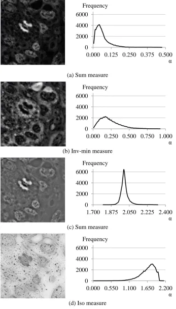
3.3 The α-image

The results of using different multifractal measures are illustrated in

Figure 3-4, and the original greyscale image is shown in Figure 3-3 for comparison.

The α-range for each measure is different: [0.0000, 0.4808] for max measure,

[0.0000, 0.9354] for inv-min measure, [1.7917, 2.3315] for sum measure, and

[0.0000, 2.1694] for Iso measure. For display purpose, the original image in

Figure 3-3 and α-images in Figure 3-4 are normalised to [0.0, 1.0], black to white.

Besides, the α-histogram for each multifractal measure shows that the distribution

of α-values has a bell-shaped curve, and is skewed and translated along the α-axis

respectively.

Figure 3-3 The greyscale image (left) and its corresponding intensity histogram (right)

0 2000 4000 6000

0.00 0.25 0.50 0.75 1.00 Frequency

(35)

24 (a) Sum measure

(b) Inv-min measure

(c) Sum measure

[image:35.595.121.469.108.716.2]

(d) Iso measure

Figure 3-4 The α-image (left) and its corresponding α-histogram (right)

0 2000 4000 6000

0.000 0.125 0.250 0.375 0.500 Frequency

α

0 2000 4000 6000

0.000 0.250 0.500 0.750 1.000 Frequency

α

0 2000 4000 6000

1.700 1.875 2.050 2.225 2.400 Frequency

α

0 2000 4000 6000

0.000 0.550 1.100 1.650 2.200 Frequency

(36)

25

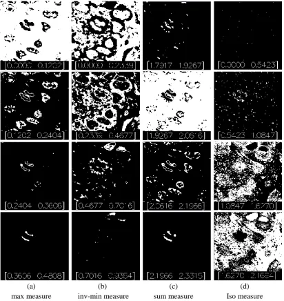
The binary images for each multifractal measure displayed in Figure 3-5 are

produced by thresholding the α-image at different α-series. These α-series represent

every quarter of the α-ranges. Only the pixels with α-values within the particular

α-series are assigned as ones and all the others as zeros. For a particular α-series

and multifractal measure, some of the tissue substances are more observable in the

binary image. Hence, image features can be detected in a particular range of the

α-values. This is a unique feature of multifractal analysis. More details are

discussed in Chapter 4.

(a) max measure

(b) inv-min measure

(c) sum measure

[image:36.595.97.510.278.715.2]

(37)

26

3.4 The Multifractal Spectrum

The following step of multifractal analysis is the calculation of fractal

dimension where sets of points have the same singularity coefficient α. Multifractal

spectrum characterises the intensity of the image; it is a unique description of the

geometric property of fractal dimension. Besides, it can be presented by plots of

fractal dimension against α-value, as shown in Figure 3-6. The resulting discrete

plot (Figure 3-6 (a)) can be displayed as a continuous function, as shown in

Figure 3-6 (b). Clearly, the latter presentation is easier to read and understand;

hence, multifractal spectrum is presented as continuous functions in this thesis.

(a) (b)

Figure 3-6 Multifractal spectrum: (a) actual form (b) continuous form

3.4.1 Fractal dimension

Theiler demonstrated that fractal dimension can be estimated using a

box-counting method, a correlation algorithm, or a fixed-mass ball technique [50].

Box counting is one of the most commonly used methods for calculating fractal

dimension [41, 45, 48] because it is simple and easy to implement. For an N by N

image, box counting only requires an average O((N2/2)logN) computation time

[49], while maintaining a good estimation for the image’s fractal dimension [51].

3.4.2 Box-counting method

Box-counting method counts the number of boxes, n(ε) with box size ε, that

contain pixels with α-values within the α-interval [αi, αi+1], as shown in Figure 3-7.

The α-intervals are obtained by subdividing the range of α-values into a

pre-specified number of sub-intervals. In this research, the number of sub-intervals 0.00

0.75 1.50

0.000 0.125 0.250 0.375 Fractal dimension

α 0.00 0.75 1.50

0.000 0.125 0.250 0.375 Fractal dimension

(38)

27

is 100. Referring to Equation 3.9, the fractal dimension, f(α), can be obtained by

calculating the slope of linear regression line of the plot of log(n(ε)) against log(ε).

The size of box ε starts from half the size of the input image of size N, and

recursively reduces until 1, as shown in Equation 3.11.

(3.9)

(3.10) , , (3.11)

(a) ε = 128 (b) ε = 64 (c) ε = 32

Figure 3-7 Box-counting method that uses different box sizes ε

3.4.3 Polynomial curve fitting

As mentioned earlier, multifractal spectrum is a discrete function of α-values;

it can be expressed as a continuous function. Representing a large set of f(x) values

by a continuous polynomial curve (see Figure 3-8 (b)) is useful for obtaining a

small set of coefficients that we can use for comparing or matching two multifractal

spectra. A general n-th order polynomial equation, f(α), is an expression which

consists of sets of variables and constants, defined as follow:

_(3.12)

where x is the variable, n is a non-negative integer, and a0, a1, a2, …, an are

(39)

28

Suppose the data points of a multifractal spectrum are the m-th pairs of

vectors, (x1, y1), (x2, y2), …, (xm, ym), where x is the value of α and y is the value of

f(α), then a least squares method can fit the spectrum to a polynomial function,

described as follow:

(3.13) (3.14) (3.15) (3.16)

The unknown coefficients a0, a1, …, an can be obtained by solving the linear

(40)

29

An example of polynomial fitting with a sixth order polynomial equation for

the multifractal spectrum (in Figure 3-6) is demonstrated in Figure 3-8. The

equation is given to be:

(3.17)

with a correlation coefficient of 0.9650.

(a) (b)

Figure 3-8 Multifractal spectrum: (a) original discrete function (b) sixth order polynomial equation

3.4.4 Adjusting the α-range

Noise often exists in digital images. A simple equalisation can minimise the

problem. As discussed in Section 3.3, the α-histogram in Figure 3-4 shows that all

α-values of the image are distributed along its unique α-range, from αmin to αmax.

Each α-interval in the α-histogram has its own count for the number of pixels with

particular α-values. The α-value can be treated as noise when its occurrence in

corresponding α-interval is below a certain threshold. In this research, the threshold

is set to 65, which is 0.1% of the total number of pixels in a 256×256 size image.

The new α-range can be modified by neglecting α-values of occurrence below the

threshold.

As shown in Figure 3-9, the α-image based on the summation measure has

α-values distributed between 1.79 and 2.33. The bold boxes in the figure show the α-intervals where the α-values have occurrence below the threshold of 65. These α-values are treated as noise and are excluded; the modified α-range is now from

0.00 0.75 1.50

0.000 0.250 0.500 f(α)

α 0.00 0.75 1.50

0.000 0.250 0.500 f(α)

(41)

30

1.90 to 2.13. Note that the α-values which located in the middle of the histogram

are not treated as noise even if its occurrence in corresponding α-interval is below

[image:41.595.100.495.416.670.2]

the threshold.

Figure 3-9 The magnified portion of the α-histogram of the sum measure from Figure 3-4

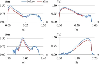
The effect of adjusting the α-range and re-sampling the spectrum is

demonstrated in Figure 3-10. It should be noted that the multifractal spectra have

similar trends as the α-histograms show in Figure 3-4. All further calculations on

multifractal spectrum will include the α-range adjustment.

(a) (b)

(c) (d)

Figure 3-10 The effect of adjusting the α-range of the multifractal spectrum for Figure 3-3 which uses the (a) max measure (b) inv-min measure (c) sum measure (d) Iso measure

0 65

1.79 1.85 1.90 1.95 2.01 2.06 2.12 2.17 2.22 2.28 Frequency

α

0.00 0.75 1.50

0.00 0.25 0.50

before after f(α)

α 0.00 0.75 1.50

0.00 0.50 1.00

f(α)

α

0.00 0.75 1.50

1.70 2.05 2.40

f(α)

α 0.00 0.75 1.50

0.00 1.10 2.20

f(α)

(42)

31

3.5 Applications in Medical Image Processing

Song et al. related electroencephalogram (EEG) signals with multifractal

theory. They compared EEG signals with rapid eye movement (REM) sleep and

four different sleep stages: awake, Stage 1, Stage 2, and slow wave sleep (SWS).

The fluctuation in signals could have correlated, uncorrelated, and anti-correlated

behaviours. Song et al. showed that EEG signals during different sleep stages could

be differentiated with multifractal measures. Human sleep EEG signals during

awaken stage, Stage 1, and REM sleep had shown anti-correlated behaviours, while

Stage 2 sleep had uncorrelated behaviour, and SWS stage had correlated behaviour.

Different sleep stages were briefly classified, and a total error rate of 41.8% was

found [52]. Therefore, Song et al. recommended that a set of scalars could better

describe human sleep EEGs rather than a single dominant scale which were

suggested in other researches.

(a) (b) (c)

(d) (e) (f)

Figure 3-11 Example of an medical image (a) original; result after: (b) Sobel operator (c) Robbers operator (d) Prewitt operator (e) Log operator (f) Hölder exponent [53]

Qi and Yu applied multifractal spectrum as an edge detection tool for a

medical computed tomography (CT) image. They compared the result with four

(43)

32

and Log operator. As shown in Figure 3-11, these operators could not precisely

display the edge information. Intact edges could not be detected with Robert, Sobel,

and Prewitt operators, while Log operator could not obtain continuous edges.

However Hölder exponent could detect exact edges with a proper selection of

multifractal spectrum threshold. Therefore, multifractal theory was concluded to be

a relatively effective method for edge detection [53].

The structure of the human retinal vessels had been proven to have

geometrical fractal properties by many literatures. Applying the fractal concepts,

Family et al. presented the first quantitative analysis on the geometry of blood

vessels in normal human retina in 1989 [54]. A year later, Mainster concluded that

fractal geometry offered a more accurate description of ocular anatomy as fractal

dimension could characterise a complete vascular patterns span over the retina [55].

Landini et al. (1995) [56] and Avakian et al. (2002) [57] pointed that the previous

work only focused on a single fractal analysis: retinal vessels might have different

properties in different regions. In 2006, T. Stosic and B. Stosic showed that human

retinal vessels have geometrical multifractal properties. Examples of retinal vessel

are illustrated in Figure 3-12. T. Stosic and B. Stosic also found that by comparing

the normal cases with pathological cases, images with pathological cases tended to

have lower generalized dimensions and have a shifted spectrum range. However,

they suggested more detailed studies were needed to explore the statistical

significance between normal and pathological cases [58].

(a) (b)

(44)

33

The time series of human brain activity could be extracted from arterial spin

labelling (ASL) Functional Magnetic Resonance Imaging (FMRI). Some

researchers focused on multifractal formalism when analysing these human brain

function. Multifractal formalism for FMRI analysis were based on two methods:

Wavelet Modulus Maxima Method (WTMM) [59] and Multifractal Detruded

Fluctuation Analysis (MF-DFA) method [60]. Shimuze et al. proposed a

multifractal FMRI analysis based on WTMM, which had high accuracy in the

scaling analysis and did not require a prior knowledge of the paradigm. However,

the extension of application on ASL function time series was limited by the

complexity of this method [61, 62]. On the other hand, Kantelhardt et al. studied

multifractal analysis which is based on MF-DFA. Although both WTMM and

MF-DFA provided similar results, Kantelhardt et al. showed that MF-DFA was

more reliable than WTMM [60]. Soares et al. used MF-DFA method and

demonstrated that the voxels from activated and non-activated brain regions

showed clear differences in the multifractal spectra [63]. The time series of human

brain activity exhibited self-similarity formalism and could be described with

multifractal spectra.

3.6 Summary of Multifractal Method

Square window is used for calculating the local singularity coefficient of the

image, and the result of the calculation is called the α-image. Four multifractal

measures are applied; each measure has its unique characteristics. Multifractal

spectrum is a function which describes the geometrical property of the α-image; it

can be estimated via box counting method. A brief flow chart to describe the

process of calculating the Hölder exponent and multifractal dimension is

(45)

[image:45.595.97.497.103.558.2]

34

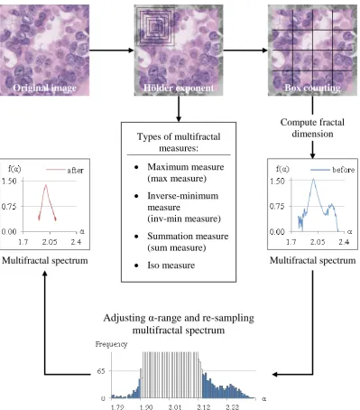
Figure 3-13 Summary of calculating the Hölder exponent and multifractal dimension

Multifractal formalism is an effective tool for biomedical image processing.

Many researchers have proposed using this technique for different medical

applications. The multifractal analysis designed for breast cancer grading is

discussed in Chapter 4.

Original image Hölder exponent Box counting

Types of multifractal measures:  Maximum measure

(max measure)  Inverse-minimum

measure

(inv-min measure)  Summation measure

(sum measure)  Iso measure

Compute fractal dimension

Multifractal spectrum Multifractal spectrum

(46)

35

Chapter 4:

System Structure and Implementation

The criteria denoted for NGS (described in Chapter 2) and multifractal theory

(defined in Chapter 3) are combined and demonstrated along with the description

of the structure for the breast cancer analysis system in this chapter.

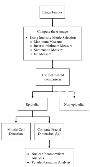
4.1 System Overview

The system overview for the multifractal analysis of breast cancer grading is

indicated in Figure 4-1. First, the image frames are loaded to the system, and the

calculation for Hölder exponent based on four multifractal measures is performed

to generate the α-images. Then, the α-threshold comparison is applied to separate

the sub-image frames of epithelial type tissues from those of non-epithelial type

tissues. Once the epithelial sub-image frames are identified, the system detects the

mitotic cells and computes the fractal spectra of the α-images. Finally, the

(47)

[image:47.595.120.426.89.654.2]

36

Figure 4-1 System overview of the multifractal analysis of the tissue images

Image Frames

Compute the α-image  Using Intensity Metric Selection

o Maximum Measure

o Inverse-minimum Measure

o Summation Measure

o Iso Measure

The α-threshold comparison

Non-epithelial Epithelial

Mitotic Cell Detection

Compute Fractal Dimension, f(α)

 Nuclear Pleomorphism Analysis

(48)

37

4.1.1

Image data extraction

The high resolution, high magnification histopathological images and data

used in this research were provided by IPAL, where 17 histopathological images

were identified and graded by pathologists. These images can be viewed with the

FrameWork Viewer, a software workstation for laboratories imaging. As shown in

Figure 4-2, pathologists can label the invasive regions, identify the mitotic cell, and

grade the invasive areas with NP and TF scores based on NGS.

Figure 4-3 shows some of the image samples, with the size of 1,024 × 1,024

pixels each, that had NP and TF scores pre-assigned by pathologists. Tissue

substances of similar types occupy a relatively small area of a section image. Hence

the identified ROIs need to be cropped into smaller sub-images. Figure 4-4 is an

example of the developed graphical user interface (GUI) program that collects the

sub-images. The GUI program was built under the OpenGL framework; more

developed visualising programs can be found in Section 4.5. The sub-images are

randomly sub-divided into smaller image frames with the size of 288 × 288 pixels

each, from the labelled invasive region of the histopathological image. Each image

frame contains a border of 16 pixels wide, which is the window size for measuring

local singularity coefficient. The sizes of the final α-images are 256 × 256 pixels

each.

Each of the 17 histopathological images contributed 150 to 250 sub-image

frames. 850 sub-image frames were non-epithelial type. 3,270 sub-image frames

were epithelial types and had NP score pre-labelled by pathologists; only 600

sub-image frames had TF score pre-labelled. The number of image frames analysed

(49)

38

(a) A view of a full slide biopsy sample

[image:49.595.96.505.102.713.2]

(b) A section view of ×5.0 zoom in

(50)

39

[image:50.595.308.494.107.683.2]

(a) (b)

(51)

40

[image:51.595.100.500.106.507.2]

Figure 4-4 The developed GUI for cropping 10 sub-image frames from a NP/TF-labelled region

Table 4-1 The number of image frames used for data analysis Score

Criterion 1 2 3 Total

NP 350 970 1,950 3,270

Algorithms for Tissue Image Analysis using Multifractal Techniques

Algorithms for

Tissue Image Analysis using

Multifractal Techniques

A thesis submitted in partial fulfilment

of the requirements for

the Degree of Master of Science

in the University of Canterbury

by

ChiangHau TAY

University of Canterbury

Abstract

Acknowledgements

Table of Contents

List of Figures

List of Tables

List of Abbreviations

Chapter 1:

Introduction

1.1 Motivation

1.2 Objectives

1.3 Publication

1.4 Thesis Overview

Chapter 2:

Background and Literature Survey

2.1 Overview of Breast Cancer Grading

2.2 Mitotic Count Scoring

2.3 Nuclear Pleomorphism Scoring

2.4 Tubule Formation Scoring

2.5 Summary of Literature Review

Chapter 3:

Multifractal Analysis

3.1 Hölder exponent

3.2 Multifractal Measures

3.3 The α-image

3.4 The Multifractal Spectrum

3.5 Applications in Medical Image Processing

3.6 Summary of Multifractal Method

Chapter 4:

System Structure and Implementation

4.1 System Overview

4.1.1