Simulation Driven Design of a Passive Liquid Cooling System for a Thermoelectric Generator

UNCORRECTED

PROOF

Applied Energy

Simulation-driven design of a passive liquid cooling system for a thermoelectric

generator

M.J. Deasy, N. Baudin, S.M. O'Shaughnessy, A.J. Robinson

Department of Mechanical & Manufacturing Engineering, Parsons Building, Trinity College Dublin, Ireland

A R T I C L E I N F O

Keywords:

Thermoelectric generator Electricity generation Natural convection Passive cooling Thermosyphon Liquid cooling

A B S T R A C T

Active cooling of thermoelectric generators (TEGs) is problematic since mechanical devices such as pumps and fans draw a high proportion of the limited power generated. Increasing the coolant fluid flow rate is typically a scenario of diminishing gains since the increased TEG power can be more than offset by the increase in power required for the fluid mover. Passive air cooling is an option, however the high air-side thermal resistance results in poor TEG power performance and low thermal efficiency. To address these issues, and others, a passive single phase liquid thermosyphon cooling system for use with TEGs has been designed, computationally simulated and experimentally tested. The novelty of the cooling system centres not only on the hot-side heat exchanger design, but also on the use of an open liquid reservoir as a dual-purposed heat store and air-side heat sink. This results in an effective source-to-sink heat exchange system that is entirely passive while providing effective cooling. This work describes the Simulation-Driven Design approach used to design the system for an example of a single TEG, experimental verification of the simulation results and TEG performance characteristics with the new cooling system.

Nomenclature

Aws wetted surface area, m⁠2

Cp specific heat capacity, J/kg K

g gravitational acceleration, m/s⁠2

Gr Grashof number,–

h fin height, m

havg average heat transfer coefficient, W/m⁠2K

k thermal conductivity, W/m K

kAl thermal conductivity, W/m K

L fin length, m

p static pressure, Pa

Pelec electrical power, W

Q heat flow to heat sink, W

Qevap heat loss due to evaporation, W

Qmanifold heat loss through manifold, W

Qpipe heat loss through pipe walls, W

Qres,sides heat loss through reservoir walls, W

q″ heat flux, W/m⁠2

Ra rayleigh number,–

RL electrical resistance of load,Ω

RTEG electrical resistance of TEG,Ω

Rth thermal resistance, K/W

s fin spacing, m

sopt optimal fin spacing, m

Tc TEG cold side temperature, K

Tfeed feed water temperature, K

Tfin,avg average fin temperature, K

Th TEG hot side temperature, K

Ths average heat sink base temperature, K

Tretn return water temperature, K

Tws heat sink wetted surface temperature, K

ΔTlm log mean temp. difference, K

ΔTTEG TEG temperature difference, K

α thermal diffusivity, m⁠2_/s

αeff effective seebeck co-efficient, V/K

β thermal expansion coefficient, 1/K

ρ density, kg/m⁠3

μ dynamic viscosity, Pa s

υ kinematic viscosity, m⁠2_/s

⁎ _{Corresponding author.}

Email address:arobins@tcd.ie (A.J. Robinson)

http://dx.doi.org/10.1016/j.apenergy.2017.07.127

UNCORRECTED

PROOF

Thermoelectric generators (TEG) are solid state semi-conductor de-vices that convert heat directly into electricity via the thermoelectric effect. Despite their low efficiency of <7%, the absence of moving parts makes TEGs reliable power generators when operated under sta-ble thermo-mechanical conditions [1]. As with any heat engine operat-ing on a thermodynamic cycle, a TEG requires both a heat source and a heat sink, with associated heat exchangers to maintain the tempera-ture differential as high as possible to maximize thermal efficiency. This study focusses on the cooling mechanisms for thermoelectric generators which can be categorised as active or passive and can use air or liquid as coolants.

Air cooled natural convection is a passive cooling technique whereby the heat is transferred directly to ambient air, with the coolant flow being driven by buoyancy forces. Generally, finned metallic heat sinks are required to dissipate the heat load in order to achieve a feasible air-side thermal resistance. Albeit a passive technique, the major draw-back of air cooled natural convective heat sinks for TEG applications is their comparatively large size compared to the TEG, with associated heat spreading and convective thermal resistances which limits cooling effectiveness and thermal efficiency. In studies such as Refs. [2–4], the TEG systems have implemented natural air cooling, however the power output is low and well below the maximum rated power. However, the excellent reliability associated with the system having no moving parts makes this solution viable for space exploration [5], automotive heat re-covery applications [6], remote power applications [7], domestic power generation [3,4], and solar power generation [8]. It is worth noting that a hybrid passive solution to improve heat spreading over the air-side fins, and thus natural air cooling effectiveness, is to employ heat pipes [9,10].

Forced air cooled systems use mechanical means, such as fans and blowers, to substantially increase the air-side convective heat transfer coefficient compared with natural convection. This results in substan-tially lower thermal resistance and a more compact form factor of the cooling system. Although the TEG thermal efficiency may increase, the power requirement for the air mover must be taken into account when considering the Coefficient of Performance (COP) of the overall TEG sys-tem, since this energy must be supplied by the TEG [11,12]. TEG system start-up also becomes problematic since the electric motors on fans and blowers have a minimum cut-in voltage. The dilemma is that the TEG may require forced air flow in order to produce the minimum cut-in voltage to run the fan/blower. This then requires an electrical store, such as a battery, in order to run the air mover during start up or times of low power generation. Fans and blowers also suffer from reliability issues due to failure of mechanical components over long term use. Re-gardless, force air systems have been investigated for domestic and in-dustrial applications [13–16], with acceptable power generation. Heat pipes have also been implemented in order to increase the area avail-able for air-side cooling and thus improve the thermal resistance and TEG power output [17].

Liquid cooled forced convection is employed for higher power TEG applications. The high convective heat transfer coefficients achieved with liquids, in particular water, can also reduce the hot-side heat sink footprint to that of the TEG [18]. However, the end-to-end sys-tem can involve many components, including a pump, remote air-side heat sink and connecting tubing and fittings which increases the over-all complexity and can adversely affect cost [1] and reliability. Posi-tively, forced liquid cooled systems can achieve power generation com-parable to the manufacturer’s specifications. Once again, however, the COP of the integrated system must be considered since electrical power is required for circulating the liquid and air-side fan, when applicable. The former is particularly relevant for compact hot-side heat exchangers

which require a high fin density to reach the target thermal resistance, which can adversely affect the required hydraulic pumping power due to increased pressure drop. Despite some shortcomings, forced liquid systems are commonly used in automotive [19,20], marine [21], indus-trial [22,23] and domestic cogeneration [24,25] applications.

An ideal cooling system for TEGs would incorporate the benefits associated with the cooling effectiveness of forced convective systems with the infinite COP and high reliability of fully passive systems. To this end, liquid cooled natural convection systems may provide an ideal engineering solution, though the published literature on this is limited. Champier et al. [26] used TEGs to cogenerate electricity and hot wa-ter from a domestic solid fuel stove with four TEGs attached directly to a reservoir of water. Initial demonstrators showed that the power gen-eration was comparatively low per module, though this was improved by using finned heatsinks on the hot-side of the liquid cooling system. Juanicóet al. [27] developed a low cost TEG system using domestic hot water radiators in a single-phase thermosyphon configuration. The sys-tem thermal-hydraulics was modelled demonstrating that syssys-tem opti-mization was realizable.

There exists few commercially available off-grid TEG power genera-tors, typically marketed for use in camping and emergency power gen-eration. Devices such as the PowerPot, FlameStower and Biolite Ket-tleCharge use a small water reservoir directly attached to a TEG, with the heat being supplied by combustion of fuel. These systems are de-signed to take advantage of the very high heat transfer coefficients asso-ciated with nucleate boiling which can maintain hot-side TEG tempera-tures in the region of 100°C. Though these devices provide a useful ser-vice and are completely passive, the performance of the TEG is greatly reduced by the high cold side temperature which reduces the thermal efficiency.

The above review illustrates that there are several methods available to provide cooling for TEG systems. The ideal system should provide ef-fective cooling and operate passively. The latter is of utmost importance since it targets the lack of parasitic electricity draw from the limited power generated by TEGs, mitigates start-up issues and improves long term reliability. These issues are addressed in this work, where a single phase water thermosyphon concept is described. Designed using Simu-lation Driven Design (SDD), the passive system uses a compact hot-side finned heat exchanger and a remote reservoir. A novel aspect of the design is that, opposed to a conventional finned air-side natural con-vection heat sink, the reservoir acts in the capacity as a gravity-pump, a thermal store and a passive heat sink in order to provide effective cold-side heat sink temperatures of the TEG over long periods of time (>10 h).

1.1. TEG theory and properties

Like any heat engine, to generate electrical energy a TEG requires heat transfer from a source of heat while simultaneously dissipated heat to a heat sink. A TEG produces power in response to a temperature dif-ference across the module. The power output not only depends on the temperature of the heat source and sink, the effectiveness of heat trans-fer to/from the TEG but also the electrical load resistance connected to the power leads of the TEG. A full thermal-electrical description of TEG behaviour can be found in [28–30] and elsewhere and will not be out-lined here for conciseness. In short, the electrical power produced by a single TEG module is expressed as;

(1)

UNCORRECTED

PROOF

load resistance, R⁠L.

The system proposed in this study is designed for operation with one TEG module, although it is likely suitable and scalable for use with multiple modules. For illustration purposes a single TEG module (TEG1B-12610-5.1) supplied by TECTEG is investigated in this study, though the cooling concept and methodology is feasible for any TEG and it is not the purpose of this investigation to test different modules. The specifications for the chosen TEG are given in Table 1.

This particular TEG is fabricated from Bismuth Telluride, which has a maximum Seebeck coefficient at∼50°C and a maximum operating temperature of 300°C. Provided the TEG is maintained below its max-imum operating temperature, a larger temperature difference will of course produce greater power, as Eq. (1) expresses. However, as the av-erage temperature of the TEG increases, the potential to produce power will also decrease. Thus, for the same temperature difference, main

Table 1 TEG specifications.

Type Bi⁠2Te⁠3

Max. hot side temperature 300°C

Dimensions 40 mm×40 mm

Open circuit voltage 7.2 V

Internal resistance 1.8Ω

Match load output voltage/current 3.6 V/2 A

Match load max. output power 7.2 W

Heat flow through the module ∼148 W

Fig. 1.Power output as a function of TEG temperature difference and average module temperature for the TEG1B-12610-5.1.

taining the TEG at a lower average temperature will generate more power, as illustrated in Fig. 1.

1.2. Design overview

This study focusses specifically on optimizing the heat dissipation, or cooling system, of a single TEG heated by a controllable heat source. The cooling mechanism predominantly relies upon natural circulation of water between the heat source and an open water reservoir. For this single phase thermosyphon system the driving force for fluid circula-tion is buoyancy. As heat energy is dissipated to the water at the source, density gradients are established which causes warmer fluid to rise and flow, via connecting tubing, to the top portion of the reservoir. Cold fluid flows downward from the bottom region of the reservoir to the heated zone to conserve mass, establishing a circulation loop between the heat source and the reservoir. At steady state, the water reservoir acts as the remote heat sink to the air, transferring the applied heat load by natural convection and free surface evaporation. This arrangement may therefore be classified as passive since it does not require electricity to operate. The cooling potential of the proposed system is investigated for both intermittent and continuous operation of the TEG.

2. Experimental apparatus

2.1. Heater block

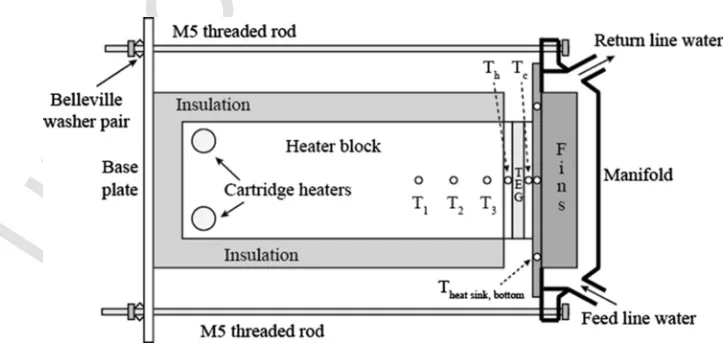
Fig. 2 shows a sketch of the heater meter bar assembly used in the experiments. It consists of an aluminium heater block of cross-section 40 mm×40 mm into which two 6 mm diameter cartridge heaters, rated at 175 W, are placed. Three 1.55 mm holes are drilled 20 mm deep into the centre of the block to accommodate K-Type 1.5 mm diameter stain-less steel sheathed grounded thermocouples. The thermocouples are lo-cated at 5 mm, 25 mm and 45 mm from the right end of the block and facilitate estimation of the temperature gradient, and thus the supplied heat flux to the surface. The arrangement of the block is such to provide one-dimensional heat conduction. The block is encased in Superwool fi-bre insulation to limit heat losses to the surroundings. Aluminium 6061 is chosen for the heater block material instead of copper. For the power levels studied here, the lower thermal conductivity of aluminium en-sures that sufficiently large temperature differences are measured along its length such that the experimental uncertainty is not excessive. The heat flux was calculated as,

(2)

UNCORRECTED

PROOF

thermocouples and k⁠Alis the aluminium thermal conductivity.

For heat sink evaluation and characterization, the heater block is at-tached directly to an aluminium heat sink, and no TEG is used in this arrangement. For evaluating the power generation using a TEG, a single module is introduced to the rig. It is held between two square copper plates, each of thickness 3 mm and side length 40 mm, used to enable the approximate TEG temperature difference to be measured. The TEG is positioned between the copper plates, which themselves are clamped between the aluminium heater block and the aluminium heat sink of the manifold.

For all experiments, clamping pressure is achieved using four M5 threaded rods. Multiple M5 Belleville washer pairs are used in series to allow for thermal expansion as the heater block is heated and cooled. This is standard practice when assembling TEG systems.

2.2. Manifold design & heat sink selection

A sketch of the assembled manifold is provided in Fig. 3. Some geo-metric constraints were applied to limit the extent of this parageo-metric study. Since the TEG under investigation is 40 mm×40 mm, the maxi-mum finned area of a heat sink must at most match this. According to Laird Technologies [31], the clamping bolts should be no further than 12 mm from the edge of the TEG where possible to ensure even pressure is applied to the module.

The manifold is manufactured from a single piece of aluminium of 30 mm thickness. A cavity of 44 mm×44 mm cross-sectional area and a depth of 27 mm is machined into the solid, which is represented by the hatched regions in Fig. 3. This enables heat sinks with fin heights ranging between 0 mm (flat plate) up to 26 mm to be included. Two holes are drilled and tapped at an angle of 30°to the outer face to ac-commodate two G1/4 male to 12 mm internal diameter barbed hose fit-tings. This angle is chosen to allow the hole to intersect with the cavity inside and to prevent the formation of air pockets which were observed to form when using horizontal connections.

The manifold provides four holes to accommodate the M5 threaded rods, Belleville washers and M5 nuts used to apply the clamping pres-sure to the TEG. The same torque (0.75 N m) is applied to each bolt us-ing a narrow range calibrated torque screwdriver.

The finned internal heat sinks are used to increase the heat transfer surface area while keeping within the cavity dimension constraints. A minimum heat sink base area of 50 mm×50 mm is required to form a

Fig. 3.Diagram of manifold and heatsink.

seal with the manifold. To create a water-tight seal, a gasket sealer was used. In this way the fins fit inside the cavity and the finned section of the heat sink occupies a maximum area of 40 mm×40 mm. For the ex-perimental investigation, an off-the-shelf aluminium heat sink is used as a baseline. The heat sink has a finned area of 40 mm×40 mm with 17 fins, 1.6 mm fin spacing and 9 mm fin height and a fin thickness of 0.7 mm. This is referred to as heat sink A throughout this study.

2.3. Flow loop configuration

A water flow loop was constructed as shown in Fig. 4. A reser-voir of water with a maximum capacity of 10 litres was connected to the heatsink manifold using two G1/4 male 12 mm internal diameter barbed hose fittings and 12 mm internal diameter braided PVC hos-ing. During experimental testing, heat is transferred from the cartridge heaters to the heater block, through the TEG if present, and onward to the aluminium heat sink. The finned heat sink dissipates the heat to the water within the manifold. Temperature differences establish buoyancy gradients within the water in the manifold which cause the warmer liq-uid to move to the upper regions and eventually out of the manifold via the return pipe back to the reservoir. Simultaneously, the water leaving the manifold via the return pipe is replaced by water entering the man-ifold via the feed pipe. The feed water is supplied by the reservoir and thus a passive, buoyancy-driven flow loop is established. This type of flow loop is also called a single phase thermosyphon.

The return and feed water temperatures are recorded at the reser-voir by K-Type 1.5 mm diameter stainless steel sheathed thermocouples. This location was chosen to ease the stress on the hose fittings in the manifold and to prevent buckling of the PVC hose. The feed and return lines were 510 mm and 540 mm in length respectively.

The purpose of the reservoir is to act as a thermal store as well as a remote air-side heat sink. The volume of water in the reservoir is such that a significant amount of heat energy must be absorbed before the feed water experiences a considerable rise in temperature. In this way the temperature difference across the thermoelectric module can be maintained at reasonable levels for sustained periods, providing that the heat input from the heater block does not greatly exceed the rec-ommended levels for the TEG. However, as the water temperature rises, heat also leaves the reservoir by natural convection at the sides and, to a greater extent, free surface evaporation at the free surface, thus dissi-pating some or all of the thermal energy supplied at the source. Evapo-ration ensures that the reservoir temperature does not rise rapidly since the evaporation rate is known to increase with the water surface tem-perature [32], which lowers its effective thermal resistance. However, this configuration means that liquid mass will be lost from the system over time so the initial volume of water must be sufficiently large if op-erating over an extended time interval.

The positioning of the reservoir relative to the manifold is crucial to the effective operation of the system. The reservoir must be located above the manifold so that a hydrostatic head is created which supplies

UNCORRECTED

PROOF

reservoir should be maintained above the fitting for the return line. If the water level drops below the fitting, the flow loop does not function as effectively. To monitor the thermal stratification of the water in the reservoir, the water temperature was recorded using thermocouples at three depths, as shown in Fig. 4.

2.4. Heat transfer data acquisition & measurement

All thermocouple measurements are acquired using a National In-struments NI-DAQ9213 16-channel thermocouple data acquisition mod-ule in conjunction with LabVIEW. In a similar manner, all voltage mea-surements are recorded using a NI-DAQ9219 module.

As suggested by Webb [33], the effective thermal resistance of the heat sink for single phase flow is determined by using the log-mean tem-perature difference,ΔT⁠lm, for a constant temperature heater surface:

(3)

In the above equation, T⁠hsrepresents the temperature of the heat sink

base. The log mean temperature difference takes into account the tem-perature difference between the feed and return water lines. This is used to calculate the thermal resistance of the heat sink, R⁠th, which is given

by Eq. (4).

(4)

Since a constant heat flux is imposed on the aluminium heat sink base and cold water enters the manifold from the bottom, the temperature distribution on the heatsink base is not uniform. To compare the simula-tions with the experiments and to calculate the performance of the heat sink, the average surface temperature of the heater is used. The maxi-mum base temperature variations ranged from 1.7°C at low heat flux to 4.3°C for the highest heat flux which is not considered excessive with regard to assuming a uniform base temperature in the use of Eqs. (3) & (4) for characterizing the thermal resistance.

2.5. Experimental procedure

Initially, the reservoir is filled with water to a level of 9.5 L. The manifold, feed and return lines are then primed with water and checked for air pockets. Subsequently, the LabVIEW data acquisition is initiated before power is supplied to the heater block by an Elektro-Automatic PS8360-10T power supply, which is also controllable from LabVIEW. The power supply to the cartridge heaters is voltage controlled. The heat flowing through the TEG is then estimated using Eq. (2) and adjusted accordingly. For each heat sink tested, three nominal heat sink heat in-puts were investigated; 60 W, 120 W and 180 W.

2.6. Uncertainty analysis

The uncertainty analysis for the heat flux and wall temperature is based on a Monte Carlo technique suggested by Kempers et al. [34]. The thermal conductivity of the heater block was calculated by aver-aging the temperature recorded by the three thermocouples, which re-sulted in an uncertainty estimated of±5%. The accuracy of the mea-sured distance between thermocouples was limited to the resolution of the measurement equipment, which was 0.1 mm. Thermocouples were calibrated against a high precision F100 RTD probe resulting in uncer-tainties of±0.2°C across the test range.

The uncertainty in heat flux decreases with increasing heat flux. The majority of the uncertainty is associated with the positioning of the tem-perature probes which thus limits the variation in the uncertainty across the different heat flux levels. Even still, the uncertainty does decrease marginally with imposed heat flux as a result of the increasing temper-ature gradient. The uncertainty in the thermal resistance is calculated to be 9%, 7% and 6% for nominal powers of 60 W, 120 W and 180 W respectively.

2.7. Heating curves

Fig. 5 plots the average heat sink base temperature together with the feed and return line temperatures for the baseline heat sink A for 60 W of input power. Immediately after heat is applied a rapid rise in the heat sink and return line temperature is observed, though the feed line tem-perature remains relatively unchanged though this stage lasts only a few minutes. Following this initial rise in heater and return line tempera-tures, a period of quasi steady behaviour, heretofore referred to as Stage 1, is observed. During Stage 1 the surface temperature as well as the feed and return line temperatures remain relatively constant. Here the reservoir is behaving as a thermal store, with the average temperature increasing (not shown) due to heating of a stratified region above the feed line port. For the 60 W case shown it takes about 1 h before the stratified layer grows to the extent that heated water reaches the feed line port. Once the stratification zone has reached the feed line, heated water is then supplied to the heat source which causes the system to enter a transient heating period where all temperatures slowly begin to increase. This transition stage can be considered one whereby the reser-voir is acting as a thermal store as well as a remote heat sink, since the some of the thermal energy is stored as sensible heat to raise the reservoir average temperature and some is dissipated to the ambient via natural convection and surface evaporation. The transition period lasts about 7 h after which steady state is reached, heretofore referred to as Stage 2. During Stage 2, the reservoir is no longer behaving as a ther-mal store per se, since the supplied energy is no longer increasing the reservoir temperature. Rather, the reservoir behaves as a remote heat sink whereby the entire heat load is dissipated to the surroundings by surface evaporation and natural convection.

3. Computational model

Simulations of the combined heat transfer and fluid flow were per-formed using Ansys Fluent 16.0. By successful comparison with the ex-perimental results, the numerical formulation allows for a wider para-meter range to be investigated, thus facilitating Simulation Driven De

UNCORRECTED

PROOF

also be analysed with detail not possible in the experiments. Within the geometric constraints of the experimental manifold, a range of fin spac-ing and fin heights were numerically investigated in order to gain an understanding of their influence on the overall heat transfer and to sub-sequently optimize for a minimum thermal resistance.

The geometry of the cooling section replicates the experimental geometry. The 3D computational domain is enclosed by the heater block, manifold outer walls, pipe inner walls, reservoir volume and the water free surface. The pipe and reservoir wall thicknesses are not mod-elled. A prescribed heat flux is supplied to a 40 mm×40 mm area on the base of the aluminium heat sink to emulate the thermal footprint of the TEG. The fluid within the heat sink, feed and return lines and reser-voir are modelled as well as that in the manifold. Since the manifold housing thermally communicates with the heated base, it partakes in the heat transfer to the enclosed liquid and this conjugate heat transfer ef-fect is taken into account. To reduce the model complexity and solution times, symmetry is assumed such that only half of the physical domain is modelled.

The computational mesh is constructed to ensure cells of equal size at the interface between the heat sink and the liquid using a shared topology approach. The cells have a minimum size of 1 mm on the boundaries of the solid/liquid interfaces and a maximum size of 3 mm elsewhere. The number of mesh elements varied based on the geometry of heat sink simulated, ranging from 6×10⁠6_{to 9×10}⁠6_{which were fine}

enough to ensure mesh independence. A sketch of a typical mesh is pro-vided in Fig. 6.

Fluid motion in the loop is initiated by buoyant natural convection. The flow is laminar in nature due to the low Grashof number as given by Eq. (5).

(5)

Buoyancy forces are included using the Boussinesq approximation, which has been used for other studies involving slow moving natural convection flows [35,36]. Fluid properties are evaluated at the av-erage liquid temperature observed in the experimental data. A small set of simulations were carried out with temperature dependent fluid properties and it was determined to have little effect on the solution, though severely increased computational time. Typical fluid properties are given in Table 2.

For incompressible, laminar, steady flow in three dimensional Carte-sian space, the governing conservation equations of continuity and mo-mentum are,

(6)

(7) In the above equationsvrepresents the velocity field, p is the static pressure,μis the dynamic viscosity and the termρg the gravitational body force. Since the flow is thermally driven there is a non-linear cou-pling with the energy equation which together dictates the temperature distribution within the fluid domain. Neglecting pressure work and ki-netic energy terms, the energy equation for an incompressible, laminar, steady flow is given as,

(8) As mentioned, the simulations consider only steady state, meaning the initial heat up and transition periods described previously and shown in Fig. 5 are not simulated. For this low speed incompressible flow problem, the segregated pressure-based solver is used with second-or-der pressure, momentum and energy discretization schemes. Simula-tions are conducted until convergence of the energy residuals is below 10⁠−6_{and momentum residuals are below 10}⁠−4_{. Integrals of the total}

rates of heat and mass transfer are also monitored to ensure conver-gence.

For the simulations, the average convective heat transfer coefficient for the aluminium heat sink is calculated using Newton’s law of cooling,

(9)

where Q is the heat supplied to the sink heat and A⁠wsrepresents the

wet-ted surface area of the heat sink. The driving temperature difference is that between the feed water temperature, T⁠feed, and the temperature

av-eraged over the wetted surface area of the heat sink, T⁠ws.

3.1. Stage 1 conditions

Stage 1 is considered a quasi-steady state since in reality it is a part of the overall transition to the final true steady state represented by Stage 2. This stage is characterized by a constant feed water ture and is simulated by a reservoir with an imposed uniform tempera-ture of 295.15 K on the side walls. The boundary types and conditions are chosen to be consistent with the experimental set up and experimen-tal observations, and are provided in Table 3.

The top surface of the reservoir is modelled with a zero shear stress condition to simulate a free surface. Heat transfer from the surface is

UNCORRECTED

PROOF

Water properties at 47.5°C.

Symbol Value Units

ρ 978.19 [kg/m⁠3_]

β 4.2×10⁠−4 _[K⁠−1_]

C⁠p 4182.00 [J/kg K]

k 0.60 [W/m K]

µ 6.1×10⁠−4 _{[kg/m s]}

Table 3

Stage 1 simulation boundary conditions.

Boundary Type Fluid Thermal

Bottom Wall No slip Adiabatic

Side Wall No slip T⁠feed

Top Wall Zero Shear h = 5 W/m⁠2_K

Pipe walls Wall No slip Adiabatic

Manifold Wall No slip Adiabatic

Heater Wall – Heat flux

Symmetry Sym – –

approximated using a heat transfer coefficient of 5 W/m⁠2_{K to ambient}

(air) at 295.15 K, which is characteristic of natural convection [37]. The heat flowing through the TEG is simulated by imposing a heat flux on the heat sink base over an area of 40 mm×40 mm. Fig. 7 shows that the manifold is supplied with cold water at the same temperature as the bulk liquid in the reservoir, with warmer fluid occupying the upper re-gion of the reservoir, representing stratified layers.

3.2. Stage 2 conditions

Stage 2 is established when thermal equilibrium with the surround-ings is reached and characterizes the ability of the reservoir to behave as a remote heat sink that dissipates the entire heat load to the ambient. The boundary types and conditions are provided in Table 4. The Stage 2 steady state is modelled with a heat transfer coefficient of 10 W/m⁠2_K

on the manifold, pipe and reservoir walls. The increase from 5 to 10 W/ m⁠2_{K is to account for the additional heat transfer due to radiation that}

occurs when the reservoir is at a higher temperature than the ambient. Using this value and the experimentally obtained temperatures, an esti-mation of the heat loss from the manifold, pipes and reservoir walls can be made.

At the top of the reservoir there is non-negligible surface evapora-tion which represents a low thermal resistance path for heat transfer. The heat loss due to evaporation is estimated from an energy balance

using Eq. (10). Heat transfer coefficients are calculated to be 60, 70 and 80 W/m⁠2_{K corresponding to heat inputs of 60 W, 120 W and 180 W}

respectively. Evaporation itself is not modelled, but replaced with this fixed heat transfer coefficient.

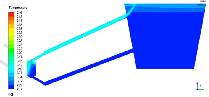
(10) Fig. 8 shows the temperature stratification in the reservoir which results in an increase in the feed water temperature when compared with Stage 1.

4. Results and discussion

4.1. Computational model verification

The experimental and numerical results were compared for heat sink A and the results are summarized in Table 5. Despite the complexity of the problem and the assumptions made to simplify the problem, good agreement is observed between the simulations and the experiments. As shown in Table 5, the agreement for the stage 1 comparisons are acceptable, though marginally outside of the experimental uncertainty. Regardless, considering that this phase is a slow transient opposed to a true steady state, the agreement is deemed satisfactory considering the assumed conditions in the model. More encouraging is the agreement between the simulations and the Stage 2 steady state of the experiments, where the agreement is within the experimental uncertainty of the mea-surements. Based on the adequate agreement between experiments and simulations, the model is considered to be adequately accurate to be used as a tool for facilitating SDD of this heat exchange system.

4.2. SDD of optimal heat sink

For a 40 mm×40 mm finned base area of fin thickness 0.7 mm, the effect of fin spacing and fin height on the heat transfer coefficient and thermal resistance were investigated using the simulation platform.

4.2.1. Effect of fin spacing

Bejan and Sciubba [38] theoretically estimate the optimum spacing in natural convection for a homogeneous fin temperature for two as-ymptotic cases discussed below:

(i) For a narrow channel in comparison to its length, the thermal boundary layers along two adjacent fins cross close to the channel inlet. As such, most of the fluid is at the same temperature. A sim-ple energy balance links the heat flux from the fin to the fluid with

UNCORRECTED

PROOF

Stage 2 simulation boundary conditions.

Boundary Type Fluid Thermal

Bottom Wall No slip Adiabatic

Side Wall No slip h = 10 W/m⁠2_K

Top Wall Zero Shear h = 60–80 W/m⁠2_K

Pipe walls Wall No slip h = 10 W/m⁠2_K

Manifold Wall No slip h = 10 W/m⁠2_K

Heater Wall – Heat flux

Symmetry Sym – –

the fluid velocity (or the Rayleigh number). In this case, the effec-tiveness increases with fin spacing since it increases the develop-ment length of the thermal boundary layers.

(ii) When the fin spacing is large relative to fin length, the thermal boundary layers can develop along the fins and never intersect. For this instance a correlation for a vertical plate with natural convec-tion can be used to correlate heat transfer to the Rayleigh number. In this situation, the effectiveness decreases when the spacing in-creases since some coolant fluid does not participate in the trans-port of heat.

From these two asymptotic scenarios an optimum spacing, s⁠opt, can

be estimated by,

(11)

where the Rayleigh number, Ra, is defined as

(12)

The constant D in Eq. (11) varies from 2 to 3 depending on the method of heating (uniform temperature or heat flux on the fin). Natural con-vection heat sinks operating in air typically have a fin spacing of ap-proximately 7 mm [39]. When using water as the working fluid the fin spacing is greatly reduced due to the higher Rayleigh numbers for simi-lar fin length and temperature differences.

Fig. 9 shows the simulated thermal resistance as a function of the fin spacing for two fin heights of 9 mm and 26 mm at a simulated heat input of 120 W. For both cases, the thermal resistance of the heat sink increases with increasing fin spacing, meaning that the simulated con-figuration corresponds to thermal boundary layers which are not mixed between the fins. Therefore these fin spacings are larger than the opti-mum, which is in agreement with earlier theories.

Fig. 10 shows the effect of fin spacing on the average heat transfer coefficient and the wetted surface area. As the footprint of the heatsink is constrained to 40 mm×40 mm, increasing the fin spacing reduces the number of fins and the wetted surface area. The heat transfer coef-ficient increases over this reduced area, however in terms of the overall performance the thermal resistance still increases as seen in Fig. 9.

The images in Fig. 11 illustrate that for the larger (3 mm) fin spacing the thermal boundary layers do not tend to merge before exiting the top of the channels. This is particularly well illustrated in the first channel on the left hand side. The main conclusion is that this spacing is sub-op-timal because the opposing boundary layers grow more or less indepen-dently for the entire length of the channel. Of course this is compounded by the fact that the larger fin spacing means there is less surface area for heat transfer. The smaller (1mm) spacing shows a quite different ther-mal profile whereby there is a therther-mal developing length after which the thermal boundary layers interact to create mixed development pro-files, where the liquid temperature notably increases along the channel length. Despite the decreasing driving temperature difference for heat transfer, the smaller fin spacing offers significantly higher surface area which more than offsets this detrimental influence.

4.2.2. Effect of fin height

Fig. 12 shows that there is an optimum fin height for which the thermal resistance of the heat sink is minimum. As the fin height in-creases the heat sink surface area also inin-creases. The thermal resistance decreases as there is a greater area over which to dissipate heat. From a practical design perspective it is interesting to note that, for this con-figuration, the thermal resistance of the heat sink does not change sub-stantially for fin heights between∼10 mm to∼25 mm.

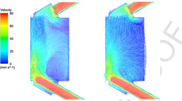
One may expect the average heat transfer coefficient to remain largely unaffected because it would be close to a 2D channel flow be-tween the fins. However, this is not the case. Fig. 13 shows the evolu-tion of both the average heat transfer coefficient and the average wall shear stress with increased fin height. When the fin height increases and therefore occupies more of the cavity within the manifold, there is more obstruction to the liquid entering the manifold from the inlet port. The geometry forces the water to recirculate as shown in Fig. 14, which de-creases the liquid velocity near the base of the heat sink and therefore the wall shear stress. Accordingly, the heat transfer coefficient also de-creases when the height fin inde-creases. These results infer that while an increase in fin height increases the surface area available for heat trans-fer, it does not have the continued benefit that reducing the fin spacing does because of the opposing influence on the heat transfer coefficient. This is because tall fins tend to block the inlet flow to a certain extent.

UNCORRECTED

PROOF

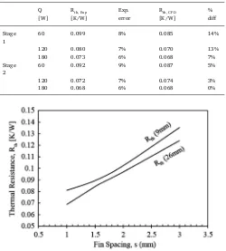
Thermal resistance of heat sink A at different heat fluxes. Q

[W] R[K/W]⁠th, Exp Exp.error R[K/W]⁠th, CFD %diff Stage

1 60 0.099 8% 0.085 14%

120 0.080 7% 0.070 13%

180 0.073 6% 0.068 7%

Stage

2 60 0.092 9% 0.087 5%

120 0.072 7% 0.074 3%

180 0.068 6% 0.068 0%

Fig. 9.Effect of fin spacing on thermal resistance for fin heights of 9 mm and 26 mm at a simulated heat input of 120 W.

Fig. 10.Effect of fin spacing on heat transfer co-efficient and wetted surface area for fin heights of 9 mm and 26 mm at a simulated heat input of 120 W.

4.3. Summary

Albeit simplified compared with the physical system, the simula-tion model encapsulates the relevant physics and complexities and ac-curately predicts experimental results. This supports the conclusion that the SDD approach is a practical tool for designing single-phase ther-mosyphon cooling hardware for TEG applications. To illustrate this the hot-side heat exchanger was investigated parametrically and the inter-play between the convective heat transfer coefficient and wetted sur-face area were detailed. For the case considered, one important finding is that the escalating surface area associated with the increasing num-ber of fins for decreasing fin spacing monotonically decreases the ther

mal resistance, despite the associated decrease in convective heat trans-fer coefficient. Thus, for the range of fin spacing investigated (1–3 mm) a small as is feasible fin spacing is ideal. The numerical study also showed that there exists an optimal fin height. However, the region of this optimum is shallow meaning that the thermal resistance is not very sensitive to fin height in the region of the optimum (between∼10 mm to∼25 mm), though increases sharply outside of this range. From an applied energy perspective this is relevant since it illustrates that care-ful attention should be paid to the design of the heat exchanger since operating outside of the optimal fin height range could negatively in-fluence the electrical power output and thermal efficiency of the TEG system. However, the SDD approach also illustrates that within the re-gion of the optimum, a range of commercially available heat sinks could be used without significantly compromising performance. In this regard, the off-the-shelf baseline heat sink A with a fin spacing of 1 mm and height of 9 mm is suitably within the ideal range that it is subsequently used to characterize the TEG system performance characteristics in the following section.

5. Thermoelectric power generation performance

To evaluate the cooling system for thermoelectric power generation, a single TEG with specifications outlined in Table 1 is installed into the experimental setup described in Section 2.3. The same experimen-tal procedure as outlined in Section 2 is followed allowing the system to reach stage 2 for each of the heater power levels tested. The rates of heat transfer through the TEG are 52 W, 105 W and 160 W respectively. An electronic resistive load (BK Precision 8540) is then connected to the TEG and operated in controlled current mode to characterize the TEG by loading it at different levels. This is found to be more stable that when attempting the same procedure in controlled resistance mode which be-comes unstable at low load resistances.

The voltage produced by the TEG was monitored throughout the ex-periment and is plotted in Fig. 15. It can be seen that the open circuit voltage, V⁠oc, is higher during Stage 1 when the feed water temperature

is close to the initial ambient temperature. Stage 2 represents long term continuous usage of a TEG whereby the water reservoir has been heated above the ambient temperature and the system reaches thermal steady state with the surroundings.

Once at steady state, the current limit is incrementally increased which changes the resistive load applied to the TEG. It is then allowed an additional 40 min to reach equilibrium since the flowing current af-fects the TEG temperature due to the Peltier, Joule and Thompson ef-fects, which combine to transport heat from the hot side to the cold side. This is shown in Fig. 16 where it is noticed that, regardless of the ther-mal power across the TEG, increasing the current causes the voltage to decrease linearly from the initial open circuit voltage. This is of course related not only to the average TEG temperature, which is found to in-crease with inin-creased current due to Joule heating, but also the dein-crease in the temperature drop across the TEG due to the action of the Peltier and Thompson effects. This means that the generated electrical power initially increases with current until a maximum is reached, after which it decreases.

UNCORRECTED

PROOF

Fig. 11.Simulated temperature distribution at 120 W heat input on a plane 5 mm from the heat sink base for 3 mm (left) and 1 mm (right) fin spacing. Isotherms represent 305 K and 310 K to illustrate entrance effects on the thermal boundary layer development.

Fig. 12.Effect of fin height on the thermal resistance for a fin spacing of 1.6 mm spacing.

Fig. 13.Effect of fin height on the heat transfer co-efficient and wall shear stress (τ).

Fig. 17. As the current is drawn the temperature difference across the TEG reduces. Thus, this characterization methodology of the TEG is more representative of practical TEG system performance.

To measure the electrical power generation over the course of a test starting from ambient conditions to Stage 2, a maximum power point tracking power converter (SPV1040) was equipped to the TEG system. The output of the power converter is set to 5 V and is connected to the electronic load set in voltage control mode to 4.7 V in order to ensure that the power converter always attempts to produce as much power as possible. The power produced over the course of the test changes due to the increasing temperature of the cold side of the TEG, as shown in Fig. 18. As this is a constant heat flux test, the temperature difference across the TEG remains constant. However the average temperature of the TEG increases and the power output thus reduces.

The difference in maximum power between Stage 1 and Stage 2 is better outlined in Table 6. It illustrates that, for the same applied power, the TEG will produce more power during Stage 1 than for Stage 2. The reason for this behaviour can be rationalized by considering Fig. 18 which plots the TEG cold side temperature and electrical power gener-ation histories for the highest thermal power test. As it is shown, Stage 1 is associated with a notably lower cold side temperature due to the reservoir being close to ambient temperature. As a result, the TEG is at a lower average temperature and thus has a lower thermal conductivity and associated higher thermal resistance which this increases tempera-ture differential and electrical power production (see Fig. 1). The table also shows that the difference is more pronounced at higher heat fluxes.

6. Conclusion

UNCORRECTED

PROOF

Fig. 15.Measured TEG open circuit voltage of the over time for three heater power set-tings.

Fig. 16.Experimental power and voltage characteristic with increasing current for the 5.1 TEG.

The cooling system is comprised of a bespoke hot-side finned heat exchanger. Simulations showed that, for the scenario and parameter range considered, (i) the fin spacing should be as low as is feasible be-cause the drop in the convective heat transfer coefficient is more than offset by the increased wetted surface area associated with a higher

Fig. 17.Effect of load current on the TEG temperature difference.

Fig. 18.TEG cold side temperature and power generated over time for a heat throughput of 160 W.

packing density of fins, and (ii) there exists an optimum fin height, though the curve is quite shallow in its region which makes the ther-mal resistance fairly insensitive to fin height over a range of ∼10 to∼25 mm.

UNCORRECTED

PROOF

Power difference between states. Electrical Power [W]

Q [W] Stage 1 Stage 2 % diff.

160 4.6 4.0 16%

105 2.8 2.5 12%

52 0.89 0.85 4%

and shown to be effective. Initially the reservoir acts as a thermal store as well as an air-side heat sink as the water is heated to the entire depth of the reservoir. Over long term use the reservoir dissipates the thermal energy to the ambient surroundings by free surface evaporation, and to a lesser extent natural convection and radiation from the container walls.

The efficacy of the simulations was verified by experimental mea-surement after which it was used to evaluate the performance of a prac-tical TEG system, including varying input power, electrical load resis-tance and maximum power point tracking. The tests showed that, for a fixed thermal power input, the TEG power output decreased with in-creased current draw as well as the inin-creased TEG cold side tempera-ture. These are related to the increase in the average temperature of the TEG module which causes its overall thermal resistance of to increase.

In summary, the entirely passive cooling system was capable of maintaining a TEG cold side temperature of∼70°C in an ambient air environment with an applied thermal power 160 W. At matched resis-tive load, the TEG that was tested produced 4.0 W, which is notably lower than the manufacturer specification of 7.2 W at 150 W of heat transfer across the TEG. In order to achieve the manufactures specifica-tions, much more aggressive liquid cooling would be required, though the required pumping power will partially or fully offset any gains in TEG power output, and this must be considered when designing such systems. The added cost and complexity as well as reliability considera-tions should also be considered is active cooling is to be considered.

Acknowledgments

The authors would like to thank Irish Aid for their continued support of this research project.

References

[1] P. Aranguren, D. Astrain, M.G. Pérez, Computational and experimental study of a complete heat dissipation system using water as heat carrier placed on a thermo-electric generator, Energy. 74 (2014) 346–358.

[2] C. Lertsatitthanakorn, Electrical performance analysis and economic evaluation of combined biomass cook stove thermoelectric (BITE) generator, Biores Technol 98 (2007) 1670–1674.

[3] R.Y. Nuwayhid, A. Shihadeh, N. Ghaddar, Development and testing of a domestic woodstove thermoelectric generator with natural convection cooling, Energy Con-vers Manage 46 (2005) 1631–1643.

[4] M.P. Codecasa, C. Fanciulli, R. Gaddi, F. Gomez-Paz, F. Passaretti, Update on the design and development of a TEG cogenerator device integrated into self-standing gas heaters, J Electron Mater (2013) 1–6.

[5] T.H. Kwan, X. Wu, Power and mass optimization of the hybrid solar panel and thermoelectric generators, Appl Energy 165 (2016) 297–307.

[6] W. He, S. Wang, L. Yue, High net power output analysis with changes in exhaust temperature in a thermoelectric generator system, Appl Energy 196 (2017) 259–267.

[7] D. Champier, Thermoelectric generators: a review of applications, Energy Convers Manage 140 (2017) 167–181.

[8] A.E.Özdemir, Y. Köysal, E.Özbaş, T. Atalay, The experimental design of solar heating thermoelectric generator with wind cooling chimney, Energy Convers Manage 98 (2015) 127–133.

[9] R.Y. Nuwayhid, R. Hamade, Design and testing of a locally made loop-type ther-mosyphonic heat sink for stove-top thermoelectric generators, Renew Energy 30 (2005) 1101–1116.

[10]

B.-J. Huang, P.-C. Hsu, R.-J. Tsai, M.M. Hussain, A thermoelectric generator using loop heat pipe and design match for maximum-power generation, Appl Therm Eng 91 (2015) 1082–1091.

[11]

S.M. O'Shaughnessy, M.J. Deasy, C.E. Kinsella, J.V. Doyle, A.J. Robinson, Small scale electricity generation from a portable biomass cookstove: prototype design and preliminary results, Appl Energy 102 (2013) 374–385.

[12]

S.M. O'Shaughnessy, M.J. Deasy, J.V. Doyle, A.J. Robinson, Adaptive design of a prototype electricity-producing biomass cooking stove, Energy Sustain Dev 28 (2015) 41–51.

[13]

D.M. Rowe, Thermoelectrics, an environmentally-friendly source of electrical power, Renew Energy 16 (1999) 1251–2125.

[14]

M.F. Remeli, L. Tan, A. Date, B. Singh, A. Akbarzadeh, Simultaneous power gener-ation and heat recovery using a heat pipe assisted thermoelectric generator system, Energy Convers Manage 91 (2015) 110–119.

[15]

L.E. Juanicó, F. Rinalde, E. Taglialavore, M. Molina, Development of a portable thermogenerator for uncontrolled heat sources, J Electron Mater 42 (2013) 1846–1854.

[16]

R. Mal, R. Prasad, V.K. Vijay, Multi-functionality clean biomass cookstove for off-grid areas, Process Saf Environ Protect: Trans Inst Chem Eng Part B. 104 (2016) 85–94.

[17]

S.M. O'Shaughnessy, M.J. Deasy, J.V. Doyle, A.J. Robinson, Field trial testing of an electricity-producing portable biomass cooking stove in rural Malawi, Energy Sus-tain Dev 20 (2014) 1–10.

[18]

A. Elghool, F. Basrawi, T.K. Ibrahim, K. Habib, H. Ibrahim, D.M.N.D. Idris, A re-view on heat sink for thermo-electric power generation: classifications and para-meters affecting performance, Energy Convers Manage 134 (2017) 260–277. [19]

S. Yu, Q. Du, H. Diao, G. Shu, K. Jiao, Start-up modes of thermoelectric generator based on vehicle exhaust waste heat recovery, Appl Energy 138 (2015) 276–290. [20]

S. Kim, S. Park, S. Kim, S.-H. Rhi, A thermoelectric generator using engine coolant for light-duty internal combustion engine-powered vehicles, J Electron Mater 40 (2011) 812.

[21]

N.R. Kristiansen, G.J. Snyder, H.K. Nielsen, Waste heat recovery from a marine waste incinerator using a thermoelectric generator, J Electr Mater 41 (2012) 124–129.

[22]

M.T. Børset,Ø. Wilhelmsen, S. Kjelstrup, O.S. Burheim, Exploring the potential for waste heat recovery during metal casting with thermoelectric generators: on-site experiments and mathematical modeling, Energy 118 (2017) 865–875. [23]

I. Savani, M.H. Waage, M. Børset, S. Kjelstrup,Ø. Wilhelmsen, Harnessing thermo-electric power from transient heat sources: waste heat recovery from silicon pro-duction, Energy Convers Manage 138 (2017) 171–182.

[24]

A.M. Goudarzi, P. Mazandarani, R. Panahi, H. Behsaz, A. Rezania, L.A. Rosendahl, Integration of thermoelectric generators and wood stove to produce heat, hot wa-ter, and electrical power, J Electron Mater 7 (2013) 2127–2133.

[25]

A. Montecucco, J. Siviter, A.R. Knox, A combined heat and power system for solid-fuel stoves using thermoelectric generators, Energy Procedia 75 (2015) 597–602.

[26]

D. Champier, J.P. Bedecarrats, M. Rivaletto, F. Strub, Thermoelectric power gener-ation from biomass cook stoves, Energy 35 (2010) 935–942.

[27]

L.E. Juanicó, F. Rinalde, E. Taglialavore, M. Molina, Development of low-cost re-mote-control generators based on BiTe thermoelectric modules, J Electron Mater 42 (2013) 1789–1795.

[28]

O. Högblom, R. Andersson, A simulation framework for prediction of thermoelec-tric generator system performance, Appl Energy 180 (2016) 472–482. [29]

C.T. Hsu, G.Y. Huang, H.S. Chu, B. Yu, D.J. Yao, An effective Seebeck coefficient obtained by experimental results of a thermoelectric generator module, Appl En-ergy (2011).

[30]

E. Brownell, M. Hodes, Optimal design of thermoelectric generators embedded in a thermal resistance network, IEEE Trans Compon Pack Manufact Technol 4 (2014) 612–621.

[31]

LairdTechnologies. Thermoelectric Handbook; 2015. [32]

E. Sartori, A critical review on equations employed for the calculation of the evap-oration rate from free water surfaces, Solar energy. 68 (2000) 77–89.

[33]

Webb R. Heat exchanger design methodology for electronic heat sinks. Frontiers in Heat and Mass Transfer (FHMT); 2011;2.

[34]

R. Kempers, P. Kolodner, A. Lyons, A. Robinson, A high-precision apparatus for the characterization of thermal interface materials, Rev Sci Instrum 80 (2009) 095111. [35]

S.M. O’Shaughnessy, A.J. Robinson, Heat transfer near an isolated hemispherical gas bubble: the combined influence of thermocapillarity and buoyancy, Int J Heat Mass Transf 62 (2013) 422–434.

[36]

S.M. O'Shaughnessy, A.J. Robinson, Convective heat transfer due to thermal Marangoni flow about two bubbles on a heated wall, Int J Therm Sci 78 (2014) 101–110.

[37]

F.P. Incropera, D.P. DeWitt, Fundamentals of heat and mass transfer, 4th ed., John Wiley & Sons, New York, 1996.

[38]

A. Bejan, E. Sciubba, The optimal spacing of parallel plates cooled by forced con-vection, Int J Heat Mass Transf 35 (1992) 3259–3264.

[39]