Bayesian Averaging of Classical Estimates in Asymmetric Vector Autoregressive (AVAR) Models

(1)

Munich Personal RePEc Archive

Bayesian Averaging of Classical

Estimates in Asymmetric Vector

Autoregressive (AVAR) Models

Albis, Manuel Leonard F. and Mapa, Dennis S.

School of Statistics, University of the Philippines Diliman

2014

Online at

https://mpra.ub.uni-muenchen.de/55902/

(2)

Bayesian Averaging of Classical Estimates in

Asymmetric Vector Autoregressive (AVAR) Models

1

Manuel Leonard F. Albis2 and Dennis S. Mapa, PhD.3

School of Statistics, University of the Philippines Diliman, Quezon City

A B S T R A C T

The estimated Vector AutoRegressive (VAR) model is sensitive to model misspecifications, such as omitted variables, incorrect lag-length, and excluded moving average terms, which results in biased and inconsistent parameter estimates. Furthermore, the symmetric VAR model is more likely misspecified due to the assumption that variables in the VAR have the same level of endogeneity. This paper extends the Bayesian Averaging of Classical Estimates, a robustness procedure in cross-section data, to a vector time-series that is estimated using a large number of Asymmetric VAR models, in order to achieve robust results . The combination of the two procedures is deemed to minimize the effects of misspecification errors by extracting and utilizing more information on the interaction of the variables, and cancelling out the effects of omitted variables and omitted MA terms through averaging. The proposed procedure is applied to simulated data from various forms of model misspecifications. The forecasting accuracy of the proposed procedure was compared to an automatically selected equal lag-length VAR. The results of the simulation suggest that, under misspecification problems, particularly if an important variable and MA terms are omitted, the proposed procedure is better in forecasting than the automatically selected equal lag-length VAR model.

Keywords: BACE, AVAR, Robustness Procedures

1

The authors are grateful to the Statistical Research and Training Center (SRTC) for the thesis fellowship grant for the completion of this study, and to the participants of the Colloquium on the Statistical Sciences at the School of Statistics, University of the Philippines, for their valuable comments.

2

Assistant Professor, School of Statistics, University of the Philippines Diliman. Email Address: [email protected]

3

(3)

9

1. Introduction

The Vector Autoregressive (VAR) model by Sims (1980) became a popular tool for

forecasting a group of interrelated economic variables because of its ease of use. However,

Braun & Mittnik (1993) showed that the ordinary least squares (OLS) coefficients VAR

estimates are sensitive to misspecification errors due to omitted variables, incorrect

lag-length, and excluded moving average (MA) terms. This results in having biased and

inconsistent estimators and creates problems in forecasting and the estimation of the impulse

response function (IRF) and variance decompositions. If these problems are not considered in

the modeling procedure, then the results of the VAR model may be misleading. A certain

degree of caution must be emphasized for the purpose of policy and decision making under

these circumstances.

The effects of excluded MA terms in the VAR model are alleviated by using a large number

of lags. However, the problem of omitting an important variable in the VAR model is the

hardest to solve. This problem is common in practice partly because of the true model is

usually unknown. .

Furthermore, the VAR model itself is misspecified. It assumes the lags of all variables in the

system are the same or symmetric. This is a problem in applied research since variables tend

to have different degrees of endogeneity. Keating (1993, 1995 & 2000) addressed this

problem by allowing unequal lag length or asymmetry in the VAR model (AVAR).

Another way of dealing with these problems is to use model averaging that is deemed to

produce robust results under problems of model misspecifications. Strachan & van Dijk

(2007) were the first to apply Bayesian Model Averaging (BMA) on VAR. The authors

assumed prior distribution for each parameter in the model. In analyzing cross-section data,

(4)

10

likelihood function of the regression model as weights in averaging the OLS estimates, where

the average is taken across all models generated in the context of the Extreme Bounds

Analysis of Leamer (1983). Sala-i-Martin, Doppelhofer & Miller (2004) formulated the

Bayesian Averaging of Classical Estimates (BACE) that uses the posterior model probability

as weights for the OLS estimates that needs only one prior information – the number of

variables in the true model.

The main objective of this paper is to develop a modeling procedure that will yield robust

VAR forecasts by the use of BACE on the forecasts of AVAR models using less assumption,

particularly on the parameter’s prior distributions of popular Bayesian VAR methods. The

combination of the two procedures, the BACE and the AVAR, is expected to minimize the

effects of misspecification errors by extracting and utilizing more information on the

interaction of the variables, and cancelling out the effects of omitted variables and omitted

MA terms through averaging. The paper also aims to determine the forecasting performance

of the BACE-AVAR method by applying it to stationary and deseasonalized vector of

variables simulated from different data characteristics. The Modified Diebold-Mariano test

and the relative MAPE will be used in the forecasting accuracy of the BACE-AVAR

procedure with respect to a model with automatic selection procedure.

2. VAR, AVAR and BACE Procedures

This section will provide a background on VAR and AVAR models, how these models are

specified and estimated, and how to measure their predictive accuracy. The BACE procedure

(5)

11

2.1 Vector Autoregressive Moving Average (VARMA) Models

Following Lütkepohl (2004), consider the generalized form of the finite order VARMA( , )

model that is given by:

∗

₌

∗ ₍₁₎

where = , … , , = 1, … , , is stationary, ∗ and ∗ are autoregressive

and moving average coefficient matrices, respectively, and = , … , ′ is a

K-dimensional white noise process, that is ! = " and

! _# = $ %&, '( = ℎ

0 + ℎ,-.'/,, (2)

and %_& is positive definite.

Due to the difficulties in estimating a VARMA , model, it is a common practice among

researchers to estimate VARMA , 0 model, which is popularly known as the VAR

model. The VAR 4 model is commonly represented by:

=

∗

₊

₍₃₎

where the terms are as defined in Equation (1). The parameters are usually estimated using

ordinary least squares (OLS) for all equations in the system.

4

The VAR operator is stable and the process is stationary if det ∗ 5 ≠ 0, where 5 ∈ ℂ. If this is the case, then the VAR( ) model can also be expressed as = ∑ :; , where : = < , if ∗ = ∗= < , and

(6)

12

Another approach in estimating the VAR model parameters is through the Bayesian VAR,

which was introduced by Litterman (1980). This approach was extensively used in modeling

and forecasting economic variables.5 The BVAR procedure involves setting the prior

distributions of the parameters and running MCMC simulations. Sun & Ni (2003; 2004)

indicated that the use of the non-informative Jeffrey’s prior in BVAR is likely to have

over-estimated posterior mean variance. Their study also showed that the results of BVAR across

different priors were different. This indicates that results of the BVAR are sensitive to the

selected prior information.

2.2 Automatic Selection Procedure

In practice, the model builder usually starts with VAR( ∗ model where ∗ is selected using

an automatic selection procedure. This involves the estimation of all VAR( model for

= 1, … , ∗_{, and selecting the initial model that yields the “best” value of a pre-selected}

information criterion. The common information criteria are the Akaike Information Criterion

(1973) that is given by:

CDE = logIJKI + 2- (4)

and the Bayesian Information Criterion by Schwarz (1978) that is of the form:

LDE = logIJKI +- log (5)

where - is the number of estimated parameters, is the number of dependent variables in the

vector, and is the sample size. Hurvich & Tsai (1993) corrected the AIC for small samples

and it has the form:

5

(7)

13

CDEM = logIJKI + 2 _{− -/ .}- (6)

Kadilar & Eldemir (2002) analyzed the performance of the popular information criteria by

simulating VAR(1) and VAR(2) models, with and without seasonality. They showed that

performance of the information criteria is better in VAR without seasonality than VAR with

seasonality. They also noted the improvement in the performance of AIC as the number of

variables in the VAR model, without seasonality, increases. However, the result for the AIC

is reversed for VAR with seasonal data. Hence, the authors recommended not to use the AIC

in the presence of seasonality in the VAR data. Overall, they ranked the performance of the

information criteria from highest to lowest as: Schwarz (SIC), Hannan-Quinn (HQ), Akaike

(AIC).

Waele & Broersen (2003) noted that the AIC is an unbiased estimate of the Kullback-Leibler

discrepancy.6 However, for a finite sample size, it tends to over-fit the model by choosing a

high number of lags, as discussed earlier. They also showed that the Kullback-Leibler

discrepancy can be used as an information criterion which they call KIC. Seghouane (2006)

proposed a refinement to the KIC, which the author called KICvc, where vc stands for vector

correction. The KICvc performs better than the KIC in model specification for small sample

sizes.

George, Sun & Ni (2004) developed a Bayesian stochastic search approach in determining

the VAR model that can incorporate restrictions on the VAR coefficients and on the elements

of the error covariance matrix. Korobilis (2010) developed an automatic variable selection

procedure using the Gibbs sampler for linear and nonlinear VARs. Numerical simulations

6

(8)

14

indicated that both procedures select a satisfactory model with improved forecasting

performance.

2.3 Asymmetric Vector Autoregressive (AVAR) Models

Hsiao (1981) was the first to suggest the estimation of VAR models with variables having

unequal lag length. However, Keating (1993) argued that Hsiao’s method depends on the

inclusion sequence of the explanatory variables in the model and that Litterman’s Bayesian

(Litterman, 1980) approach gives biased parameter estimates, a minor issue in forecasting

but a potential problem in determining macroeconomic structures. Keating introduced

asymmetries in the lag lengths of the variables in the VAR system and named this as

Asymmetric VAR (AVAR) model. The AVAR( , … _Q), can be written as

=

R

∗ ∗

+

(7)

where ∗ = max { , _W, … , _Q}; R = diag{1_{{ Z} _[_}, 1_{{ Z} _\_}, … , 1_{{ Z} _]_}}, a diagonal matrix

having indicator variables as elements such that 1_{^ Z} _{_}_` = {1 '( ' ≤ ₌; 0 + ℎ,-.'/,}; the

rest are as previously described. The Rmatrix restricts some of the parameters to zero and

this matrix introduces the inequalities in the lag-length of the variables.

The AVAR model is a VAR model that permits unequal lag length for the variables in the

equations. However, the lag specification should be the same across all equations in the

system. Because of this, the AVAR gives a parsimonious model with a substantial reduction

in the standard errors compared to the ordinary VAR. This translates to the clarity in the

interpretations from the impulse response function and variance decompositions.

Keating also performed an automatic selection procedure over a set of AVAR models. For a

(9)

15

number of lags c, and for each estimated model, the selected information criterion is

computed. The best AVAR model with the best information criterion is selected. There are cQ

number of AVAR models needed to be estimated in the procedure. For convenience, the

values of the AIC, SIC and HQ that are computed using Keating’s procedure will be called

KAIC, KSIC and KHQ respectively.7

Ozcicek & McMillin (1999) studied the performance of the popular information criteria, such

as AIC, SIC, KAIC and KSIC, in determining the lag length of a VAR model. Using a

variety of autoregressive data structure such as either short or long-lagged process, and

symmetric and asymmetric lag lengths, the authors showed that AIC is best for symmetric

data, since the other information criteria under-fits the model. The authors also showed that

KAIC is the best criterion to use for asymmetric data and they proposed this criterion to be

used in modeling since the lag length structure of the data is uncertain and most of the time

asymmetric in theory.

2.4 Predictive Accuracy

Diebold and Mariano (1995) developed a test for predictive accuracy in forecasting that is not

restricted to the quadratic loss function and can handle a wide variety of error characteristics.

For the two forecasts {d }e and {d_W }e for the series { }e , let {, }e and {,_W }e

be the associated forecast errors. The loss associated with a forecast at time is given by the

loss function f , d and the authors pointed out that the loss function is a direct

function of the forecast errors, that is, f , d = f , . The null hypothesis of the

Diebold-Mariano test is ! g = 0, where g = f , − f ,_W is the loss differential. So

7

(10)

16

that if we have {g }e , then under the assumption that the loss differential series is

covariance stationary and short memory,

√ ig̅ − kl→ oi0,2p(m _m 0 l, (8)

where, g̅ =

e∑ ge and (m 0 =Wq∑;t ;rm s , the spectral density of the loss

differential at frequency zero, having r_m s = !{ g − k g _t− k} , the sample

autocovariance of the loss differential to lag s, and k is the population mean of the loss

differential.

Harvey, Leybourne and Newbold (HLN) (1997) corrected the Diebold-Mariano (DM) test for

finite samples. The ℎ-step ahead forecasts DM test statistic is given by:

uv = g̅wxyig̅lz W ₍₉₎

where xyig̅l is the estimated variance of g̅ that is given by

xyig̅l ≈1|rd + 2 rdQ #

Q

} ₍₁₀₎

and, rd_Q is the estimated autocovariance of g̅ that has the form:

rdQ= 1 g − g̅ g Q− g̅ e

Q~ (11)

The ℎ-step ahead forecasts Modified DM test (MDM) is of the form:

vuv = • + 1 − 2ℎ + ℎ ℎ − 1 €Wuv (12)

having a Student’s distribution with − 1 degrees of freedom. The MDM test statistic was

(11)

17

forecasting performance of the VAR model that is selected automatically using an

information criterion.

The Mean Absolute Percentage Error (MAPE) is a descriptive measure of predictive accuracy

that is given by:

vC•! = 1 ‚ − d ‚

e

(13)

where |⋅| is the absolute value function. The MAPE was used in the study to measure the

distance between the actual and predicted forecasts. The ratio of two MAPE is called the

relative MAPE and is given by the form

…,†vC•! =_vC•!vC•!_∗ (14)

where vC•! is from the ' # model and vC•!∗ is from the baseline model. Relative MAPE

of less than 1 implies that the model that is being evaluated is better than the baseline model.

2.5 Bayesian Averaging of Classical Estimates

The BACE by Sala-i-Martin, et. al. (2004) computes the weighted average of the OLS

coefficient estimates weighted by the probability that the model where it is estimated from is

the true model. This approach also has an advantage over BMA, since it only needs the

number of variables in the model as prior information under the assumption of equal prior

inclusion probabilities for each variable, whereas the BMA must be given assumed prior

distributions for all of the parameters.

The procedure involves estimating all regression models of the form

(12)

18

where ‰ is the variable of interest, Œ is a vector of fixed variables that appear in all the

regressions, and Ž₌ ∈ • is a vector of variables taken from the • collection of all other

variables under consideration.

If it is assumed that the prior inclusion probability of each variable in the model are equal, the

prior probability of model ?, denoted as •iv₌l, will be:

•iv=l = ‘’“” Q_

‘1 −’“” Q_ (16)

where ’“ is the speculated number of variables in the true model, is the total number of

variables in the dataset, and ’₌ is the number of variables in the ? # model.

The weights that will be used in the averaging is the posterior probabilities of the v₌′/. The

weight is a function of the prior probability and is given by:

•iv=| l = •iv=l•

Q_/W ––!

= —/W

∑ • v •W] Q˜/W ––! —/W (17)

where the ––!₌ is the sum of squared errors in model ?. Therefore, the posterior mean of Š is

given by:

! Š| = •iv=I lŠK= W™

=

(18)

where ŠK₌ is the estimated value of the vector of coefficients under OLS; and its

corresponding posterior variance is of the form:

xš- Š| = •iv=I lxš- Š| , v= W]

=

+ •iv=I lwŠK=− ! Š| zW W]

=

(13)

19

3. The BACE-AVAR Procedure

In specifying the AVAR model, the procedure of Keating (1995) estimates c AVAR models

given a maximum lag length of c that is set by the researcher. The best specification will be

selected based on the model that gives the best value of an information criterion.

The prior probability •i ₌l will be assumed to be equal for all the equations in the ? #

estimated VAR model. The formula for the prior probability for the AVAR model ₌ is

given by:

•i =l = ›c†₌œ ‘_c”†̅ •_

‘1 −_c”†̅ ž •_ (20)

where, †₌ is the total number of AR lag regressors for each of the equations in the ? # model,

and †̅ is the assumed total number of lags of all the variables in the true model. To simplify

the procedure, the value for †̅ can be given by running an automatic selection procedure over

VAR models and setting †̅ based on the recommended number of lags. Alternatively, the

researcher may run BACE-AVAR using a different †̅.

The formula for the posterior probability will be:

•iv₌ | l = •i =l •_/W ––!=

e/W

∑ •ž™ •˜/W ––! e/W (21)

where ––!₌ is the sum of squared errors of the AVAR model that is given by ––!₌ =

∑Q ∑e Q − dQ W .8 This will give a single weight for an estimated AVAR model

depending on the ability of all its equations to fit their corresponding variables.

8

(14)

20

3.1 BACE-AVAR on Forecasted Values

The posterior probabilities will also be used in computing for the forecasts of the

BACE-AVAR procedure. The forecasts will be the weighted mean of the forecast series produced by

the AVAR models, with the posterior probabilities as its weights. The + # forecast for

the vector of variables _e~ from the BACE-AVAR procedure is given by:

e~

¡¢£¤

₌

_¥

= =,e~

ž™

=

(22)

where d_=,e~ is the forecast at time + of the ? # AVAR model, and ¥₌ is as discussed

above. The corresponding standard error of ¡¢£¤_e~ is the average of the standard errors of the

AVAR forecasts that is given by the formula

/,

¡¢£¤e~

=

¥

=

w/,i

=,e~

lz

ž™

= (23)

3.2 Summary of the Procedure

For a ’-dimensional vector of stationary time-series variables in , the procedure of the

Bayesian Averaging of Classical Estimates in Asymmetric Vector Autoregressions

(BACE-AVAR) is as follows:

1. Set c and †̅, the maximum lag length for the AVAR models and the assumed

symmetric lag length of the models. The †̅ can be set by using the automatic selection

procedures for VAR models given a certain information criterion. c may be set as

c = †̅ + 3, as adding a constant 3 to the lag length as specified by an automatic

(15)

21

2. Estimate all possible AVAR models given c using OLS. The total number of models

to be estimated is c .

3. For each of these models, compute the prior probability •i ₌l and the posterior

probability •i ₌| l that the ? # AVAR model has the correct specification.

4. For each model, obtain the forecasts along with their variances.

5. Compute the weighted forecasts and its corresponding variance at time , _e~¡¢£¤ and

/, ¡¢£¤e~ .

3.3 Performance of BACE-AVAR through Simulations

The performance of BACE-AVAR was assessed using simulations. A 3-dimensional vector

time-series dataset9 was generated from a VAR or VARMA; for that particular dataset, all

possible AVAR models were estimated given a maximum number of lags c, as well as their

corresponding posterior probabilities of being the true model; the impulse responses and

variable forecasts were weighted using these posterior model probabilities, and the results

were compared with the true impulse response function and true forecasted values,

respectively. The forecasting performance of the method was compared to the symmetric

VAR that is selected by AIC for the cases with sample size 1000 and AICc for the other

cases. The number of iterations for each case was set to 100.

9

(16)

22 3.3.1 Specific Scenarios

The data were generated arbitrarily with the restriction that the time-series is stable and

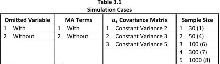
non-stationary. The BACE-AVAR was evaluated using cases summarized in Table 3.1. Overall,

[image:16.595.108.489.303.415.2]

sixty scenarios were considered.

Table 3.1 Simulation Cases

Omitted Variable MA Terms _§ Covariance Matrix Sample Size

1 With 1 With 1 Constant Variance 2 1 30 (1) 2 Without 2 Without 2 Constant Variance 3 2 50 (4) 3 Constant Variance 5 3 100 (6)

4 300 (7)

5 1000 (8)

3.3.1.1 Sample Size

The range for the sample size is from 30 to 1000. The choice of range for the sample size is

mainly due to the periodicity of the data that is being used in practice. A sample size of 30

can be viewed as an annual data; a sample size of 50, as quarterly data; a sample size of 100

as a monthly data; a sample size of 300 can be viewed as weekly data; and 1000 can be

associated to daily data. Though these specifications were a generalization of common

practice, the BACE-AVAR procedure does not limit the sample size with respect to the

periodicity of the data. It is just more likely in practice that the sample size of the data is

directly related to the period of the series, that is, higher sampling rate will have a larger

(17)

23

Furthermore, data collected on lower sampling rates have a higher amount of aggregated

information than higher frequency samples. In mimicking this phenomenon, the AR part of

the true model will have a lag order that is directly related to the sample size that will be

obtained. The AR lag orders are enclosed in parenthesis beside the sample sizes in Table 3.1.

3.3.1.2 Covariance Matrix

Three cases will be set for the covariance matrix % of the innovation series =

• , ¨ , ˆ ′, or = _• , _¨ , _ˆ , _‹ ′, in the case of an omitted variable. These will be

limited to a diagonal matrix with equal elements, which were set to be two, three and five,

that is, Σ = ' ∗ I , ' ∈ {2, 3, 5} and ∈ {3, 4}. These values for the scalar covariance matrix

were chosen to determine the performance of the BACE-AVAR procedure through different

magnitudes of variances, relative to the performance of the automatically selected model.The

starting values of the simulated data and the parameters for each replicate will be the same in

order to have comparable results for the different specification of %.

3.3.1.3 Omitted Moving Average Terms

The case wherein there is an omitted MA term was also considered in the simulations. The

MA term are restricted to lag order of one. The MA terms will be omitted in the modeling

procedure.

3.3.1.4 Omitted Variable

It is likely in practice that some of the important variables in the system were not included in

the modeling. It may be because that the variable is difficult to measure, the variable has not

been measured, or the variable cannot be measured directly. In simulating this phenomenon, a

(18)

24

will be used in modeling. The AR and/or MA parameters of this omitted variable will be

generated using the same procedure as the parameter generation of the variables of interest.

4. Results & D i s c u s s i o n

This chapter discusses the performance of the BACE-AVAR procedure in forecasting and in

determining the interaction of the variables given some misspecification errors. The problems

that were encountered in the simulation proper will be discussed first. The discussion of the

results will then follow. In summary, the BACE-AVAR procedure has an advantage in

forecasting over the automatically selected model under the problem of an omitted important

variable and excluded MA term.

4.1 Preliminary Concerns on the Simulation

The formula for the posterior probability of the BACE procedure in cross-section data given

Equation (17) involves the ––! being raised to the power −•/2, where • is the sample size

of the cross-section data. In the BACE-AVAR procedure, the resulting posterior probability

will be zero for a large sample size due to the small size of the ––!. Therefore, the problem

was counteracted by raising the ––! to − 0.1 /2 on this part of the formula that is given in

Equation (21) for the sample sizes = 300 and = 1000 since any power of the ––! that is

less than −100/2 yields undefined posterior probabilities. However, this stands only as a

temporary remedy to the problem. This issue posits that the order in which the ––! converges

in the formula of the posterior probability may be different, in time-series data, from

(19)

25

There were cases wherein the steps taken in order to have a simulated data that is stable and

stationary do not work, since the generated parameters were selected at random. In order to

guarantee a model that gives a stable data, a data burning of 10,000 time points were done.

Table 4.1 gives the lag length of the symmetric VAR models in the simulation. The number

of AVAR models for models with lower lag length is small because c = †̅ + 3. This may

affect the results of the averaging and may decrease the performance of the BACE-AVAR on

smaller samples. Therefore, the performance for small samples of the BACE-AVAR

procedure as stated in the results of the simulation may still be further improved.

Table 4.1

Average VAR Lag Lengths from Automatic Selection Procedure Using AICc

Sample Size No Omitted Variable With an Omitted Variable No MA Term With MA Term No MA Term With MA Term

30 (1) 1.03 1.36 1.07 1.33

50 (4) 3.02 3.46 2.44 2.86

100 (6) 5.66 6.27 4.85 5.4

300 (7) 7.04 8.93 7.27 8.64

1000* (8) 8.07 12.79 11.25 13.79

* AIC for Sample Size 1000

4.2 Forecasting Accuracy

This section will discuss the results of the forecasting accuracy of the BACE-AVAR

procedure relative to the automatically selected model having the least value of AIC for large

samples and least value of AICc for small samples, which will be hereafter called MINIC. In

determining the forecasting accuracy of the procedures, the MDM test and the MAPE were

(20)

26 4.2.1 Modified Diebold-Mariano Test

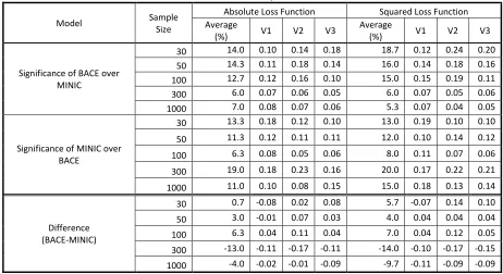
The results for the forecasting accuracy are given in Table 4.2 and Table 4.3. The tables

present the proportion of significant MDM test result at 10% level of significance that the

BACE-AVAR procedure has a better measure of forecasting accuracy than the MINIC, and

vice versa, for the different sample sizes, and by the loss functions that were used. The

differences of the proportion of significant tests between the BACE-AVAR and the MINIC

were also reported, as well as the average proportion of significant MDM tests for the

variables of interest. The MDM test result for each of the variable of interest is given in

Appendix A. Generally, the results of the MDM test indicate that the BACE-AVAR

procedure is better than the MINIC in forecasting under the omitted variable problem. The

BACE-AVAR procedure performs the same with respect to the MINIC across the different

variance specification. This indicates that the BACE-AVAR procedure is not affected by the

variance specification as specified in the simulations, relative to the automatically selected

model.

In Table 4.2, for the case of no omitted variable and no omitted MA term, the BACE-AVAR

is slightly better than the MINIC for small samples ( = 30, 50 š•g 100 . However, its

performance diminished for sample sizes where the posterior model probability was

modified. For = 1000, the forecasting accuracy of MINIC over the BACE-AVAR

procedure is about 25%. For the case of no omitted variable but with an omitted MA term,

the results indicate similar outcome as the previous case, but the improvement of the MINIC

over the BACE-AVAR procedure now comes with smaller magnitude.

Table 4.2

MDM Test: Proportion of Significance for the Case of No Omitted Variable Alpha: 0.10; Number of Iterations: 100

Model Sample Size

(21)

27 Significance

of BACE over MINIC

30 14.3 15.7 14.0 18.7

50 16.0 15.0 14.3 16.0

100 10.7 11.3 12.7 15.0

300 4.3 6.0 6.0 6.0

1000 3.3 5.3 7.0 5.3

Significance of MINIC over BACE

30 10.0 13.3 13.3 13.0

50 5.7 6.7 11.3 12.0

100 10.3 12.3 6.3 8.0

300 22.3 22.3 19.0 20.0

1000 26.3 31.7 11.0 15.0

Difference (BACE-MINIC)

30 4.3 2.3 0.7 5.7

50 10.3 8.3 3.0 4.0

100 0.3 -1.0 6.3 7.0

300 -18.0 -16.3 -13.0 -14.0

1000 -23.0 -26.3 -4.0 -9.7

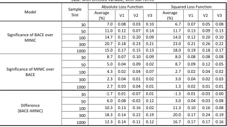
In Table 4.3, for the case of an omitted variable with no excluded MA term, the

BACE-AVAR procedure has better forecasting accuracy than the MINIC except for = 30.

Furthermore, the magnitude of this improvement increases as the sample size increases. The

improvement of the BACE-AVAR procedure drastically increases for sample sizes involving

the modified posterior probability. For the case of omitting an important variable and MA

term, the BACE-AVAR is better than the MINIC in terms of forecasting accuracy at around

15% to 20% depending on the sample size. The results emphasize that more information can

still be extracted by the BACE-AVAR procedure for small samples by improving the weights

or the posterior model probability.

Increasing the level of significance to 5% as stated in Tables A.2.1 to A.2.4 in Appendix A,

yields the same interpretation that the MINIC is better than the BACE-AVAR procedure

when there are no misspecification errors. In addition to this, the outputs also show that the

result is reversed when there are misspecification errors. Increasing the level of significance

(22)

28

of one procedure over the other may just be deemed as negligible due to the small values of

[image:22.595.101.494.214.472.2]

the significant percentages. Full results are given in Appendix A.

Table 4.3

MDM Test: Proportion of Significance for the Case of an Omitted Variable Alpha: 0.10; Number of Iterations: 100

Model Sample Size

No MA Term With MA Term Absolute Loss Squared Loss Absolute Loss Squared Loss Significance

of BACE over MINIC

30 5.7 7.0 7.0 6.7

50 10.7 10.3 11.0 11.7

100 7.7 9.3 14.7 14.0

300 19.3 17.7 20.7 23.0

1000 16.3 20.7 15.0 18.0

30 11.7 11.3 8.7 8.0

50 5.0 6.0 5.0 8.7

100 5.0 6.0 4.3 2.7

300 2.3 2.0 2.3 3.0

1000 2.0 2.0 2.7 1.3

30 -6.0 -4.3 -1.7 -1.3

50 5.7 4.3 6.0 3.0

100 2.7 3.3 10.3 11.3

300 17.0 15.7 18.3 20.0

1000 14.3 18.7 12.3 16.7

4.2.2 Mean Absolute Percentage Error

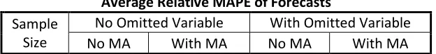
The forecasting accuracy was also measured descriptively by the relative MAPE. The relative

MAPE forecasts of the BACE-AVAR procedure with respect to the MAPE forecasts of the

MINIC are given in Table 4.4 and Appendix B. Relative MAPE values that are less than one

imply that the BACE-AVAR forecasts are closer to the outsample data than the MINIC,

whereas values greater than one indicate the opposite.

Table 4.4

Average Relative MAPE of Forecasts Sample

Size

[image:22.595.143.455.722.761.2]

(23)

29 30 0.6195 0.6390 1.0007 0.7803

50 0.7221 1.3715 0.9521 1.1204 100 1.1456 0.7054 1.2131 1.3044 300 0.5876 0.6308 0.4813 0.6042 1000 0.7547 1.5094 0.5429 0.7231

The result in Table 4.4 for the case of no omitted variable and no omitted MA term reveals

that the forecasts of the BACE-AVAR procedure using the unmodified posterior probability

are closer to the actual values compared to the forecasts of the MINIC by about 35% except

for the sample size 50. For the case of = 300 š•g 1000, the BACE-AVAR procedure also

has the same performance over the MINIC. This indicates that even if the MDM test suggests

that the MINIC is superior to the BACE-AVAR for cases of no misspecification, the

forecasts of BACE-AVAR are closer to the actual values than the forecasts of the MINIC on

the average.

For the case of no omitted variable but with an omitted MA term, it seems that the forecasts

of the BACE-AVAR procedure is closer to the outsample data than that of the MINIC by

about 35% except for = 50. The result still holds for the cases of the modified posterior

probability except for = 1000. Thus, the BACE-AVAR procedure is, on the average, still

at par or better in some cases than the MINIC based on the relative MAPE.

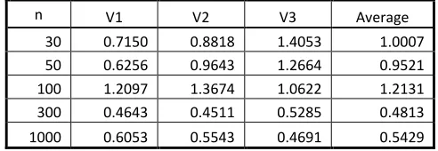
The BACE-AVAR procedure is better than or at par to the MINIC for the case wherein an

important variable is omitted. The relative MAPE of BACE-AVAR to the MAPE of the

MINIC reaches around 0.50 for the sample size of 1000 – a 50% improvement over the

MINIC. All the relative MAPE of the sample sizes that were subjected to the modified

posterior probability are less than one. This result is not contained only for the sample size of

300 and 1000 but is also evident for = 300, except for = 100, that exhibits a relative

(24)

30

not be a linear function of the sample size. Nevertheless, it is evident that the BACE-AVAR

procedure can reach a 50% improvement over the MINIC in terms of MAPE forecasts.

For the case of an omitted variable and excluded MA term, the BACE-AVAR procedure

improves over the MINIC for = 30, 300 š•g 1000. The relative MAPE for the sample

size 50 and 100 is 1.12 and 1.30, respectively. Furthermore, the improvement of the MINIC

over the BACE-AVAR procedure exhibits an upward trend from the sample size of 30 to

100, which are the sample sizes that use the original form of the posterior model probability.

This may imply that correction on the posterior probability may also be applied to improve

the overall performance of the BACE-AVAR procedure. Full results are given in Appendix

B.

5. Conclusion

Misspecification problems in VAR modeling such as incorrect AR lag, excluded MA terms,

and omitted relevant variables, are common in practice. The worst problem among those that

were stated is omitting an important variable since it is immeasurable given the data on hand.

Aside from that, it also gives biased and inconsistent estimates. The implication of this

problem is crucial in policy evaluation since it will yield misleading forecasts and incorrect

variable relationships.

This study presents the application of the BACE on AVAR models in forecasting in presence

of misspecification errors. Simulations under different scenarios were done to evaluate the

performance of the BACE-AVAR procedure over an automatically selected model using an

information criterion.

The results suggest that the BACE-AVAR procedure produces more accurate forecasts than

(25)

31

variables and omitted MA term. The forecasting accuracy of the BACE-AVAR procedure is

better for large sample sizes. On the other hand, if there are no omitted variable and excluded

MA term, the automatically selected model is better than the BACE-AVAR procedure. Given

the results of the study, the BACE-AVAR procedure is recommended in forecasting.

It is recommended to simulate the performance of the BACE-AVAR procedure for processes

generated from a structural VAR. It is also recommended to extend the BACE-AVAR

procedure for cointegrated variables. But before working on these recommendations, it is

suggested to improve the posterior model probability in order for the BACE-AVAR

procedure to be at par with the automatically selected model when there is no

(26)

32

B i b l i o g r a p h y

Akaike, H. (1973). A New Look at the Statistical Model Identification. IEEE Transactions on Automatic Control, Vol. 19(No. 6), pp. 716-723.

Akaike, H. (1974, Dec.). A new look at the statistical model identification. Automatic Control, IEEE Transactions on, Vol. 19(No. 6), pp. 716,723.

Braun, P. A., & Mittnik, S. (1993, Oct.). Misspecifications in vector autoregressions and their effects on impulse responses and variance decompositions. Journal of Econometrics, Vol. 59(No. 3), pp. 319-241.

Carriero, A., Kapetanios, G., & Marcellino, M. (2009). Forecasting Exchange Rates with a Large Bayesian VAR. International Journal of Forecasting, pp. 400-417.

Chen, A.-S., & Leung, M. T. (2003). A Bayesian Vector Error Correction Model in Forecasting Exchange Rates. Computers and Operations Research, Vol. 30, pp. 887-900.

Diebold, F. X., & Roberto, M. S. (1995, July). Comparing Predictive Accuracy. Journal of Business & Economic Statistics, Vol. 13(No. 3), pp. 253-263.

Fackler, J. S., & Krieger, S. C. (1986, Jan). An Application of Vector Time Series Techniques to Macroeconomic Forecasting. Journal of Business & Economic Statistics, Vol. 4(No. 1), pp. 71-80.

Hannan, E. J., & Quinn, B. G. (1979). The Determination of the Order of an Autoregression. Journal of the Royal Statistical Society. Series B (Methodological), Vol. 41(No. 2), pp. 190-195.

Harvey, D., Leybourne, S., & Newbold, P. (1997). Testing the Equality of Prediction Mean Squared Errors. International Journal of Forecasting, Vol. 13, pp. 281-291.

Hsiao, C. (1981). Autoregressive Modelling and Money-Income Causality Detection. Journal of Monetary Economics, Vol. 7(No. 1), pp 85-106.

Hurvich, C. M., & Tsai, C.-L. (1993). A Corrected Akaike Information Criterion for Vector Autoregressive Model Selection. Journal of Time Series Analysis, Vol. 14(No. 3), pp. 271-279.

Jorda, O. (2005, March). Estimation and Inference of Impulse Responses by Local Projections. The American Economic Review, Vol. 95(No. 1), pp. 161-182.

Kadilar, C., & Erdemir, C. (2002). Comparison of Performance Among Information Criteria in VAR and Seasonal VAR models. Hacettepe Journal of Mathematics and Statistics, Vol. 31, pp. 127-137.

Keating, J. W. (1993). Asymmetric Vector Autoregression. Proceedings of the Business and Economic Statistics Section (pp. pp. 68-73). American Statistical Association.

(27)

33

Keating, J. W. (2000). Macroeconomic Modeling with Asymmetric Vector Autoregressions. Journal of Macroeconomics, Vol. 22(No. 1), pp. 1-28.

Korobilis, D. (2010, March 4). VAR forecasting using Bayesian variable selection. Retrieved January 24, 2011, from Munich Personal RePec Archive: http://mpra.ub.uni-muenchen.de/21124/

Kullback, S., & Leibler, R. A. (1951). On Information and Sufficiency. Annals of Mathematical Statistics, Vol. 22(No. 1), pp. 79-86.

Leamer, E. E. (1983, March). Let's Take the Con Out of Econometrics. The American Economic Review, Vol. 73(No. 1), pp. 31-43.

Litterman, R. B. (1980). A Bayesian Procedure for Forecasting With Vector Autoregressions.

Working Paper.

Lütkepohl, H. (1990, Feb. ). Asymptotic Distributions of Impulse Response Functions and Forecast Error Variance Decompositions of Vector Autoregressive Models. The Review of Economics and Statistics, Vol. 72(No. 1), pp. 116-125.

Lütkepohl, H. (2004). Forecasting with VARMA Models. Department of Economics, European University Institute.

Ng, S., & Pierre, P. (2001, Nov.). Lag Length Selection and the Construction of Unit Root Tests with Good Size and Power. Econometrica, Vol. 69(No. 6), pp. 1519-1554.

Ozcicek, O., & McMillin, W. D. (1999, April). Lag length selection in vector autoregressive models: symmetric and asymmetric lags. Applied Economics, Vol. 31(No. 4), pp. 517-524.

Po, H. H., Chi, H. W., Shyu, J., & Hsiao, C. Y. (2002). A Litterman BVAR approach for production forecasting of technological industries. Technological Forecasting and Social Change, Vol.70, pp. 67-82.

Ramos, F. F. (2003). Forecasts of market shares from VAR and BVAR models: a comparison of their accuracy. International Journal of Forecasting, Vol. 19, pp. 95-100.

Runkle, D. E. (1987, Oct.). Vector Autoregressions and Reality. Journal of Business and Economic Statistics, Vol. 5(No. 4), pp. 437-42.

Sala-I-Martin, X. X. (1997, May). I Just Ran Two Million Regressions. The American Economic Review, Vol. 87(No. 2), pp. 178-183.

Sala-I-Martin, X., Doppelhofer, G., & Miller, R. (2004, September). Determinants of Long-Term Growth: A Bayesian Averaging of Classical Estimates (BACE). The American Economic Review, Vol. 94(No. 4), pp. 813-835.

Schwartz, G. (1978). Estimating the Dimension of a Model. Annals of Statistics, Vol. 6(No. 2), pp. 461-464.

(28)

34

Seghouane, A.-K. (2006, Oct.). Vector Autoregressive Model-Order Selection From Finite Samples Using Kullback’s Symmetric Divergence. Circuits and Systems I: Regular Papers, IEEE Transactions on, Vol. 53(No. 10), pp. 2327-2335.

Shibata, R. (1980). Asymptotically efficient selection of the order of the model for estimating parameters in a linear process. Annals of Statistics, Vol. 8(No. 1), pp. 147-146.

Sims, C. A. (1980). Comparison of Interwar and Postwar Business Cycles: Monetarism Reconsidered.

The American Economic Review: Papers and Proceedings of the Ninety-Second Annual Meeting of the American Economic Association.Vol. 70, No. 2, pp. pp. 250-257. American Economic Association.

Sims, C. A. (1980, Jan). Macroeconomics and Reality. Econometrica, Vol. 48(No. 1), pp. 1-48.

Sims, C. A., & Zha, T. (1999, Sep.). Error Bands for Impulse Responses. Econometrica, Vol. 67(No. 5), pp. 1113-1155.

Stock, J. H., & Watson, M. W. (1996, Jan.). Evidence on Structural Instability in Macroeconomic Time Series Relations. Journal of Business & Economic Statistics, Vol. 14(No. 1), pp. 11-30.

Stock, J. H., & Watson, M. W. (2001). Vector Autoregressions. The Journal of Economic Perspective, Vol. 15(No. 4), pp. 105-115.

Strachan, R., & van Dijk, H. K. (2007). Bayesian Model Averaging in Vector Autoregressive Processes with an Investigation of Stability of the US Great Ratios and Risk of a Liquidity Trap in the USA, UK and Japan. MRG Discussion Paper Series 1407.

Sun, D., & Ni, S. (2004). Bayesian analysis of vector-autoregressive models with noninformative priors. Journal of Statistical Planning and Inference, Vol. 121, pp. 291-309.

Tsay, R. S. (2005). Analysis of Financial Time Series (Second Edition ed.). Hoboken, New Jersey: John Wiley & Sons, Inc.

Waele, S. d., & Broersen, P. M. (2002, Oct.). Finite sample effects in vector autoregressive modelling.

Instrumentation and Measurement, IEEE Transactions on, Vol. 51(No. 5), pp. 917-992.

Waele, S. d., & Broersen, P. M. (2003, Feb.). Order Selection for Vector Autoregressive Models.

(29)

35

APPENDIX A

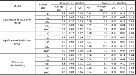
[image:29.595.71.528.153.403.2]

M D M T e s t : P r o p o r t i o n o f S i g n i f i c a n c e

Table A.1.1

Alpha: 0.10; Number of Iterations: 100 Case: No Omitted Variable; No MA Terms

Model Sample

Size

Absolute Loss Function Squared Loss Function Average

(%) V1 V2 V3

Average

(%) V1 V2 V3

Significance of BACE over MINIC

30 0.15 0.13 0.15 15.7 0.14 0.13 0.20 0.15

50 0.18 0.15 0.15 15.0 0.16 0.15 0.14 0.18

100 0.11 0.13 0.08 11.3 0.10 0.16 0.08 0.11

300 0.06 0.05 0.02 6.0 0.08 0.07 0.03 0.06

1000 0.01 0.03 0.06 5.3 0.05 0.05 0.06 0.01

30 0.12 0.10 0.08 13.3 0.14 0.16 0.10 0.12

50 0.08 0.04 0.05 6.7 0.10 0.06 0.04 0.08

100 0.07 0.12 0.12 12.3 0.09 0.15 0.13 0.07

300 0.23 0.22 0.22 22.3 0.21 0.27 0.19 0.23

1000 0.28 0.26 0.25 31.7 0.33 0.32 0.30 0.28

30 0.03 0.03 0.07 2.3 0.00 -0.03 0.10 0.03

50 0.10 0.11 0.10 8.3 0.06 0.09 0.10 0.10

100 0.04 0.01 -0.04 -1.0 0.01 0.01 -0.05 0.04

300 -0.17 -0.17 -0.20 -16.3 -0.13 -0.20 -0.16 -0.17 1000 -0.27 -0.23 -0.19 -26.3 -0.28 -0.27 -0.24 -0.27

Table A.1.2

Alpha: 0.10; Number of Iterations: 100 Case: No Omitted Variable; With MA Terms

Model Sample

Size

(%) V1 V2 V3

Average

(%) V1 V2 V3

30 14.0 0.10 0.14 0.18 18.7 0.12 0.24 0.20

50 14.3 0.11 0.18 0.14 16.0 0.14 0.18 0.16

100 12.7 0.12 0.16 0.10 15.0 0.15 0.19 0.11

300 6.0 0.07 0.06 0.05 6.0 0.07 0.05 0.06

1000 7.0 0.08 0.07 0.06 5.3 0.07 0.04 0.05

30 13.3 0.18 0.12 0.10 13.0 0.19 0.10 0.10

50 11.3 0.12 0.11 0.11 12.0 0.10 0.14 0.12

100 6.3 0.08 0.05 0.06 8.0 0.11 0.07 0.06

300 19.0 0.18 0.23 0.16 20.0 0.17 0.22 0.21

1000 11.0 0.10 0.08 0.15 15.0 0.18 0.13 0.14

30 0.7 -0.08 0.02 0.08 5.7 -0.07 0.14 0.10

50 3.0 -0.01 0.07 0.03 4.0 0.04 0.04 0.04

100 6.3 0.04 0.11 0.04 7.0 0.04 0.12 0.05

300 -13.0 -0.11 -0.17 -0.11 -14.0 -0.10 -0.17 -0.15

[image:29.595.66.528.466.718.2]

(30)

[image:30.595.71.528.107.360.2]

36

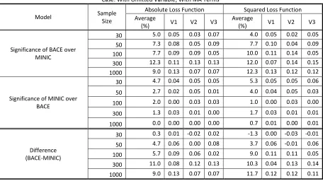
Table A.1.3

Alpha: 0.10; Number of Iterations: 100 Case: With Omitted Variable; No MA Terms

Model Sample

Size

(%) V1 V2 V3

Average

(%) V1 V2 V3

30 5.7 0.09 0.03 0.05 7.0 0.11 0.06 0.04

50 10.7 0.07 0.10 0.15 10.3 0.10 0.11 0.10

100 7.7 0.08 0.09 0.06 9.3 0.08 0.11 0.09

300 19.3 0.14 0.22 0.22 17.7 0.15 0.20 0.18

1000 16.3 0.17 0.15 0.17 20.7 0.23 0.21 0.18

30 11.7 0.11 0.09 0.15 11.3 0.09 0.10 0.15

50 5.0 0.09 0.04 0.02 6.0 0.09 0.06 0.03

100 5.0 0.07 0.04 0.04 6.0 0.10 0.05 0.03

300 2.3 0.04 0.01 0.02 2.0 0.03 0.01 0.02

1000 2.0 0.03 0.01 0.02 2.0 0.02 0.02 0.02

30 -6.0 -0.02 -0.06 -0.10 -4.3 0.02 -0.04 -0.11

50 5.7 -0.02 0.06 0.13 4.3 0.01 0.05 0.07

100 2.7 0.01 0.05 0.02 3.3 -0.02 0.06 0.06

300 17.0 0.10 0.21 0.20 15.7 0.12 0.19 0.16

1000 14.3 0.14 0.14 0.15 18.7 0.21 0.19 0.16

Table A.1.4

Alpha: 0.10; Number of Iterations: 100 Case: With Omitted Variable; With MA Terms

Model Sample

Size

(%) V1 V2 V3

Average

(%) V1 V2 V3

30 7.0 0.08 0.03 0.10 6.7 0.07 0.05 0.08

50 11.0 0.12 0.07 0.14 11.7 0.13 0.09 0.13

100 14.7 0.15 0.20 0.09 14.0 0.12 0.20 0.10

300 20.7 0.18 0.23 0.21 23.0 0.21 0.26 0.22

1000 15.0 0.17 0.15 0.13 18.0 0.19 0.18 0.17

30 8.7 0.07 0.10 0.09 8.0 0.08 0.08 0.08

50 5.0 0.04 0.09 0.02 8.7 0.09 0.12 0.05

100 4.3 0.02 0.04 0.07 2.7 0.02 0.04 0.02

300 2.3 0.04 0.01 0.02 3.0 0.04 0.02 0.03

1000 2.7 0.03 0.04 0.01 1.3 0.02 0.01 0.01

30 -1.7 0.01 -0.07 0.01 -1.3 -0.01 -0.03 0.00

50 6.0 0.08 -0.02 0.12 3.0 0.04 -0.03 0.08

100 10.3 0.13 0.16 0.02 11.3 0.10 0.16 0.08

300 18.3 0.14 0.22 0.19 20.0 0.17 0.24 0.19

[image:30.595.71.528.434.690.2]

(31)

[image:31.595.63.528.106.361.2]

37

Table A.2.1

Model Sample

Size

(%) V1 V2 V3

Average

(%) V1 V2 V3

30 10.0 0.11 0.08 0.11 11.0 0.11 0.10 0.12

50 9.3 0.10 0.10 0.08 8.7 0.08 0.09 0.09

100 6.3 0.06 0.09 0.04 7.3 0.08 0.11 0.03

300 2.0 0.04 0.02 0.00 4.0 0.06 0.04 0.02

1000 1.0 0.00 0.00 0.03 2.0 0.02 0.01 0.03

30 8.0 0.08 0.08 0.08 7.7 0.09 0.08 0.06

50 2.7 0.04 0.02 0.02 3.7 0.04 0.04 0.03

100 5.0 0.04 0.07 0.04 6.7 0.05 0.08 0.07

300 16.3 0.17 0.17 0.15 16.0 0.19 0.14 0.15

1000 21.0 0.23 0.19 0.21 21.0 0.19 0.22 0.22

30 2.0 0.03 0.00 0.03 3.3 0.02 0.02 0.06

50 6.7 0.06 0.08 0.06 5.0 0.04 0.05 0.06

100 1.3 0.02 0.02 0.00 0.7 0.03 0.03 -0.04

300 -14.3 -0.13 -0.15 -0.15 -12.0 -0.13 -0.10 -0.13 1000 -20.0 -0.23 -0.19 -0.18 -19.0 -0.17 -0.21 -0.19

Table A.2.2

Model Sample

Size

(%) V1 V2 V3

Average

(%) V1 V2 V3

30 9.7 0.07 0.08 0.14 12.0 0.05 0.18 0.13

50 9.0 0.07 0.09 0.11 10.3 0.10 0.08 0.13

100 9.7 0.10 0.13 0.06 9.0 0.10 0.12 0.05

300 3.0 0.03 0.04 0.02 3.7 0.04 0.01 0.06

1000 3.7 0.05 0.02 0.04 3.0 0.05 0.02 0.02

30 9.0 0.12 0.07 0.08 9.7 0.13 0.07 0.09

50 7.7 0.07 0.09 0.07 7.7 0.07 0.09 0.07

100 4.3 0.08 0.02 0.03 3.3 0.07 0.02 0.01

300 12.0 0.11 0.15 0.10 12.3 0.14 0.13 0.10

1000 8.0 0.08 0.08 0.08 7.7 0.09 0.07 0.07

30 0.7 -0.05 0.01 0.06 2.3 -0.08 0.11 0.04

50 1.3 0.00 0.00 0.04 2.7 0.03 -0.01 0.06

100 5.3 0.02 0.11 0.03 5.7 0.03 0.10 0.04

300 -9.0 -0.08 -0.11 -0.08 -8.7 -0.10 -0.12 -0.04

[image:31.595.72.528.438.690.2]

(32)

[image:32.595.73.527.106.359.2]

38

Table A.2.3

Model Sample

Size

(%) V1 V2 V3

Average

(%) V1 V2 V3

30 3.0 0.07 0.01 0.01 3.7 0.09 0.01 0.01

50 8.0 0.05 0.09 0.10 6.3 0.05 0.08 0.06

100 3.7 0.02 0.05 0.04 5.3 0.06 0.04 0.06

300 9.3 0.08 0.11 0.09 9.3 0.07 0.12 0.09

1000 11.0 0.14 0.10 0.09 9.3 0.11 0.09 0.08

30 7.7 0.07 0.07 0.09 6.0 0.05 0.07 0.06

50 2.3 0.04 0.03 0.00 3.0 0.05 0.02 0.02

100 3.3 0.06 0.01 0.03 3.0 0.04 0.02 0.03

300 1.7 0.02 0.01 0.02 2.0 0.03 0.01 0.02

1000 1.0 0.02 0.00 0.01 0.7 0.00 0.00 0.02

30 -4.7 0.00 -0.06 -0.08 -2.3 0.04 -0.06 -0.05

50 5.7 0.01 0.06 0.10 3.3 0.00 0.06 0.04

100 0.3 -0.04 0.04 0.01 2.3 0.02 0.02 0.03

300 7.7 0.06 0.10 0.07 7.3 0.04 0.11 0.07

1000 10.0 0.12 0.10 0.08 8.7 0.11 0.09 0.06

Table A.2.4

Model Sample

Size

(%) V1 V2 V3

Average

(%) V1 V2 V3

30 5.0 0.05 0.03 0.07 4.0 0.05 0.02 0.05

50 7.3 0.08 0.05 0.09 7.7 0.10 0.04 0.09

100 7.7 0.09 0.09 0.05 10.0 0.11 0.14 0.05

300 12.3 0.11 0.13 0.13 12.0 0.07 0.14 0.15

1000 9.0 0.13 0.07 0.07 12.3 0.13 0.12 0.12

30 4.7 0.04 0.05 0.05 5.3 0.05 0.05 0.06

50 2.7 0.02 0.05 0.01 4.0 0.04 0.05 0.03

100 2.0 0.00 0.03 0.03 1.0 0.00 0.03 0.00

300 1.3 0.03 0.01 0.00 1.7 0.03 0.01 0.01

1000 0.0 0.00 0.00 0.00 0.7 0.01 0.00 0.01

30 0.3 0.01 -0.02 0.02 -1.3 0.00 -0.03 -0.01

50 4.7 0.06 0.00 0.08 3.7 0.06 -0.01 0.06

100 5.7 0.09 0.06 0.02 9.0 0.11 0.11 0.05

300 11.0 0.08 0.12 0.13 10.3 0.04 0.13 0.14

[image:32.595.71.527.434.690.2]

(33)

[image:33.595.63.527.106.361.2]

39

Table A.3.1

Model Sample

Size

(%) V1 V2 V3

Average

(%) V1 V2 V3

30 4.7 0.06 0.03 0.05 5.7 0.06 0.04 0.07

50 4.0 0.06 0.03 0.03 4.0 0.06 0.03 0.03

100 1.3 0.01 0.02 0.01 2.0 0.02 0.03 0.01

300 0.7 0.02 0.00 0.00 1.0 0.02 0.01 0.00

1000 0.0 0.00 0.00 0.00 0.0 0.00 0.00 0.00

30 4.7 0.03 0.05 0.06 4.3 0.04 0.03 0.06

50 1.0 0.01 0.01 0.01 1.0 0.02 0.01 0.00

100 2.7 0.04 0.02 0.02 2.0 0.04 0.02 0.00

300 8.0 0.10 0.07 0.07 7.0 0.08 0.07 0.06

1000 7.3 0.10 0.04 0.08 5.0 0.06 0.04 0.05

30 0.0 0.03 -0.02 -0.01 1.3 0.02 0.01 0.01

50 3.0 0.05 0.02 0.02 3.0 0.04 0.02 0.03

100 -1.3 -0.03 0.00 -0.01 0.0 -0.02 0.01 0.01

300 -7.3 -0.08 -0.07 -0.07 -6.0 -0.06 -0.06 -0.06

1000 -7.3 -0.10 -0.04 -0.08 -5.0 -0.06 -0.04 -0.05

Table A.3.2

Model Sample

Size

(%) V1 V2 V3

Average

(%) V1 V2 V3

30 4.7 0.02 0.06 0.06 6.0 0.04 0.07 0.07

50 4.7 0.05 0.04 0.05 4.0 0.03 0.03 0.06

100 2.3 0.02 0.04 0.01 2.3 0.04 0.02 0.01

300 1.0 0.01 0.02 0.00 1.7 0.01 0.01 0.03

1000 1.0 0.01 0.00 0.02 1.3 0.03 0.00 0.01

30 5.7 0.07 0.04 0.06 6.0 0.08 0.04 0.06

50 5.7 0.05 0.07 0.05 4.3 0.04 0.06 0.03

100 0.7 0.02 0.00 0.00 1.0 0.01 0.01 0.01

300 4.3 0.07 0.05 0.01 4.3 0.06 0.05 0.02

1000 2.3 0.00 0.03 0.04 2.3 0.03 0.02 0.02

30 -1.0 -0.05 0.02 0.00 0.0 -0.04 0.03 0.01

50 -1.0 0.00 -0.03 0.00 -0.3 -0.01 -0.03 0.03

100 1.7 0.00 0.04 0.01 1.3 0.03 0.01 0.00

300 -3.3 -0.06 -0.03 -0.01 -2.7 -0.05 -0.04 0.01

[image:33.595.72.528.438.690.2]

(34)

[image:34.595.70.528.107.360.2]

40

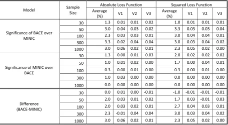
Table A.3.3

Model Sample

Size

(%) V1 V2 V3

Average

(%) V1 V2 V3

30 1.0 0.02 0.00 0.01 0.7 0.01 0.00 0.01

50 2.7 0.02 0.03 0.03 2.3 0.02 0.03 0.02

100 1.3 0.01 0.01 0.02 0.7 0.00 0.01 0.01

300 3.7 0.01 0.06 0.04 1.7 0.02 0.03 0.00

1000 3.0 0.04 0.03 0.02 3.0 0.05 0.03 0.01

30 2.3 0.01 0.02 0.04 3.0 0.02 0.04 0.03

50 0.0 0.00 0.00 0.00 0.0 0.00 0.00 0.00

100 1.7 0.03 0.00 0.02 1.7 0.03 0.01 0.01

300 0.7 0.01 0.01 0.00 0.0 0.00 0.00 0.00

1000 0.0 0.00 0.00 0.00 0.0 0.00 0.00 0.00

30 -1.3 0.01 -0.02 -0.03 -2.3 -0.01 -0.04 -0.02

50 2.7 0.02 0.03 0.03 2.3 0.02 0.03 0.02

100 -0.3 -0.02 0.01 0.00 -1.0 -0.03 0.00 0.00

300 3.0 0.00 0.05 0.04 1.7 0.02 0.03 0.00

1000 3.0 0.04 0.03 0.02 3.0 0.05 0.03 0.01

Table A.3.4

Model Sample

Size

(%) V1 V2 V3

Average

(%) V1 V2 V3

30 1.3 0.01 0.01 0.02 1.0 0.01 0.01 0.01

50 3.0 0.04 0.03 0.02 3.3 0.03 0.03 0.04

100 2.3 0.03 0.03 0.01 3.0 0.04 0.04 0.01

300 3.3 0.02 0.04 0.04 3.0 0.03 0.04 0.02

1000 3.0 0.06 0.02 0.01 2.3 0.05 0.02 0.00

30 1.3 0.00 0.01 0.03 2.0 0.02 0.02 0.02

50 1.0 0.01 0.02 0.00 1.7 0.00 0.04 0.01

100 0.3 0.00 0.01 0.00 0.3 0.00 0.01 0.00

300 1.0 0.03 0.00 0.00 0.0 0.00 0.00 0.00

1000 0.0 0.00 0.00 0.00 0.0 0.00 0.00 0.00

30 0.0 0.01 0.00 -0.01 -1.0 -0.01 -0.01 -0.01

50 2.0 0.03 0.01 0.02 1.7 0.03 -0.01 0.03

100 2.0 0.03 0.02 0.01 2.7 0.04 0.03 0.01

300 2.3 -0.01 0.04 0.04 3.0 0.03 0.04 0.02

[image:34.595.72.528.438.689.2]

(35)

41

APPENDIX B

R e l a t i v e M A P E o f F o r e c a s t s

[image:35.595.174.419.171.257.2]

MAPE(BACE-AVAR)/MAPE(MINIC)

Table B.1

Case: No Omitted Variable; No MA Term

n V1 V2 V3 Average

30 0.4684 0.6977 0.6924 0.6195

50 0.6220 0.7342 0.8100 0.7221

100 0.6338 1.4573 1.3457 1.1456

300 0.6588 0.5710 0.5329 0.5876

[image:35.595.174.419.316.400.2]

1000 0.6678 0.7614 0.8349 0.7547

Table B.2

Case: No Omitted Variable; With MA Term

n V1 V2 V3 Average

30 0.6718 0.6824 0.5628 0.6390

50 2.1923 1.0767 0.8456 1.3715

100 0.2722 0.7403 1.1038 0.7054

300 0.3998 0.8795 0.6133 0.6308

1000 2.6022 0.9538 0.9723 1.5094

Table B.3

Case: With Omitted Variable; No MA Term

n V1 V2 V3 Average

30 0.7150 0.8818 1.4053 1.0007

50 0.6256 0.9643 1.2664 0.9521

100 1.2097 1.3674 1.0622 1.2131

300 0.4643 0.4511 0.5285 0.4813

1000 0.6053 0.5543 0.4691 0.5429

Table B.4

Case: With Omitted Variable; With MA Term

n V1 V2 V3 Average

30 0.5468 0.5716 1.2224 0.7803

50 1.2342 1.1004 1.0267 1.1204

100 1.4864 1.2833 1.1436 1.3044

300 1.1347 0.3448 0.3331 0.6042

[image:35.595.174.420.458.543.2] [image:35.595.175.418.598.683.2]