Parallel Active Learning: Eliminating Wait Time with Minimal Staleness
Robbie Haertel, Paul Felt, Eric Ringger, Kevin Seppi
Department of Computer Science Brigham Young University
Provo, Utah 84602, USA
[email protected], [email protected],
[email protected], [email protected]
http://nlp.cs.byu.edu/
Abstract
A practical concern for Active Learning (AL) is the amount of time human experts must wait for the next instance to label. We propose a method for eliminating this wait time inde-pendent of specific learning and scoring al-gorithms by making scores always available for all instances, using old (stale) scores when necessary. The time during which the ex-pert is annotating is used to train models and score instances–in parallel–to maximize the recency of the scores. Our method can be seen as a parameterless, dynamic batch AL algo-rithm. We analyze the amount of staleness introduced by various AL schemes and then examine the effect of the staleness on perfor-mance on a part-of-speech tagging task on the Wall Street Journal. Empirically, the parallel AL algorithm effectively has a batch size of one and a large candidate set size but elimi-nates the time an annotator would have to wait for a similarly parameterized batch scheme to select instances. The exact performance of our method on other tasks will depend on the rel-ative ratios of time spent annotating, training, and scoring, but in general we expect our pa-rameterless method to perform favorably com-pared to batch when accounting for wait time.
1 Introduction
Recent emphasis has been placed on evaluating the effectiveness of active learning (AL) based on re-alistic cost estimates (Haertel et al., 2008; Settles et al., 2008; Arora et al., 2009). However, to our knowledge, no previous work has included in the
cost measure the amount of time that an expert an-notator must wait for the active learner to provide in-stances. In fact, according to the standard approach to cost measurement, there is no reason not to use the theoretically optimal (w.r.t. a model, training proce-dure, and utility function) (but intractable) approach (see Haertel et al., 2008).
In order to more fairly compare complex and time-consuming (but presumably superior) selec-tion algorithms with simpler (but presumably in-ferior) algorithms, we describe “best-case” (mini-mum, from the standpoint of the payer) and “worst-case” (maximum) cost scenarios for each algorithm. In the best-case cost scenario, annotators are paid only for the time they spend actively annotating. The worst-case cost scenario additionally assumes that annotators are always on-the-clock, either annotat-ing or waitannotat-ing for the AL framework to provide them with instances. In reality, human annotators work on a schedule and are not always annotating or waiting, but in general they expect to be paid for the time they spend waiting for the next instance. In some cases, the annotator is not paid directly for wait-ing, but there are always opportunity costs associ-ated with time-consuming algorithms, such as time to complete a project. In reality, the true cost usually lies between the two extremes.
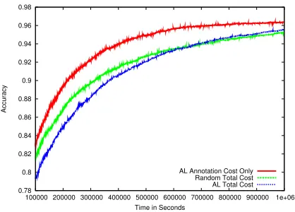
However, simply analyzing only the best-case cost, as is the current practice, can be misleading, as illustrated in Figure 1. When excluding waiting
time for a particular selection algorithm1 (“AL
An-notation Cost Only”), the performance is much
bet-1
0.78 0.8 0.82 0.84 0.86 0.88 0.9 0.92 0.94 0.96 0.98
100000 200000 300000 400000 500000 600000 700000 800000 900000 1e+06
Accuracy
Time in Seconds
[image:2.612.87.296.65.215.2]AL Annotation Cost Only Random Total Cost AL Total Cost
Figure 1: Accuracy as a function of cost (time). Side-by-side comparison of best-case and worst-case cost measurement scenarios reveals that not ac-counting for the time required by AL to select in-stances affects the evaluation of an AL algorithm.
ter than the cost of random selection (“Random Total Cost”), but once waiting time is accounted for (“AL Total cost”), the AL approach can be worse than ran-dom. Given only the best-case cost, this algorithm would appear to be very desirable. Yet, practition-ers would be much less inclined to adopt this al-gorithm knowing that the worst-case cost is poten-tially no better than random. In a sense, waiting time serves as a natural penalty for expensive selection algorithms. Therefore, conclusions about the use-fulness of AL selection algorithms should take both best-case and worst-case costs into consideration.
Although it is current practice to measure only best-case costs, Tomanek et al. (2007) mention as a desideratum for practical AL algorithms the need for what they call fast selection time cycles, i.e., algo-rithms that minimize the amount of time annotators wait for instances. They address this by employing the batch selection technique of Engleson and Da-gan (1996). In fact, most AL practitioners and re-searchers implicitly acknowledge the importance of wait time by employing batch selection.
However, batch selection is not a perfect solution. First, using the tradtional implementation, a “good” batch size must be specified beforehand. In research, it is easy to try multiple batch sizes, but in practice where there is only one chance with live annotators, specifying a batch size is a much more difficult prob-lem; ideally, the batch size would be set during the
process of AL. Second, traditional methods use the same batch size throughout the entire learning pro-cess. However, in the beginning stages of AL, mod-els have access to very little training data and re-training is often much less costly (in terms of time) than in the latter stages of AL in which models are trained on large amounts of data. Intuitively, small batch sizes are acceptable in the beginning stages, whereas large batch sizes are desirable in the latter stages in order to mitigate the time cost of training. In fact, Haertel et al. (2008) mention the use of an increasing batch size to speed up their simulations, but details are scant and the choice of parameters for their approach is task- and dataset-dependent. Also, the use of batch AL causes instances to be chosen without the benefit of all of the most recently
anno-tated instances, a phenomenon we callstalenessand
formally define in Section 2. Finally, in batch AL, the computer is left idle while the annotator is work-ing and vice-verse.
We present a parallel, parameterless solution that can eliminate wait time irrespective of the scoring
alogrithm and training method. Our approach is
based on the observation that instances can always be available for annotation if we are willing to serve instances that may have been selected without the benefit of the most recent annotations. By having the computer learner do work while the annotator is busy annotating, we are able to mitigate the effects of using these older annotations.
The rest of this paper will proceed as follows: Section 2 defines staleness and presents a progres-sion of four AL algorithms that strike different bal-ances between staleness and wait time, culminat-ing in our parallelized algorithm. We explain our methodology and experimental parameters in Sec-tion 3 and then present experimental results and compare the four AL algorithms in Section 4. Con-clusions and future work are presented in Section 5.
2 From Zero Staleness to Zero Wait
We work within a pool- and score-based AL setting in which the active learner selects the next instance
from an unlabeled pool of dataU. A scoring
func-tionσ (aka scorer) assigns instances a score using
a modelθtrained on the labeled dataA; the scores
Input: A seed set of annotated instancesA, a set of pairs of unannotated instances and their initial scoresS, scoring functionσ, the candidate set sizeN, and the batch sizeB
Result:Ais updated with the instances chosen by the AL process as annotated by the oracle
whileS 6=∅do 1
θ←TrainModel(A) 2
stamp← |A|
3
C ←ChooseCandidates(S,N) 4
K ← {(c[inst], σ(c[inst], θ))|c∈ C}
5
S ←S−C∪K 6
T ←pairs fromKwithc[score]in the topB 7
scores
fort∈T do 8
S ← S −t 9
staleness← |A| −stamp; // unused 10
A ← A ∪Annotate(t) 11
end 12
end 13
Algorithm 1:Pool- and score-based active learner.
an unerring oracle provides the annotations. These concepts are demonstrated in Algorithm 1.
In this section, we explore the trade-off between staleness and wait time. In order to do so, it is bene-ficial to quantitatively define staleness, which we do
in the context of Algorithm 1. After each modelθ
is trained, a stamp is associated with thatθthat
indi-cates the number of annotated instances used to train it (see line 3). The staleness of an item is defined to be the difference between the current number of items in the annotated set and the stamp of the scorer that assigned the instance a score. This concept can be applied to any instance, but it is particularly in-formative to speak of the staleness of instances at the time they are actually annotated (we will simply refer to this as staleness, disambiguating when nec-essary; see line 10). Intuitively, an AL scheme that chooses instances having less stale scores will tend to produce a more accurate ranking of instances.
2.1 Zero Staleness
There is a natural trade-off between staleness and the amount of time an annotator must wait for an
instance. Consider Algorithm 1 whenB = 1and
N = ∞ (we refer to this parameterization as
ze-rostale). In line 8, a single instance is selected for
annotation (|T |= B = 1); the staleness of this
in-stance is zero since no other annotations were pro-vided between the time it was scored and the time it was removed. Therefore, this algorithm will never select stale instances and is the only way to guaran-tee that no selected instances are stale.
However, the zero staleness property comes with a price. Between every instance served to the an-notator, a new model must be trained and every in-stance scored using this model, inducing potentially large waiting periods. Therefore, the following op-tions exist for reducing the wait time:
1. Optimize the learner and scoring function (in-cluding possible parallelization)
2. Use a different learner or scoring function
3. Parallelize the scoring process
4. Allow for staleness
The first two options are specific to the learning and scoring algorithms, whereas we are interested in re-ducing wait time independent of these in the general AL framework. We describe option 3 in section 2.4; however, it is important to note that when train-ing time dominates scortrain-ing, the reduction in waittrain-ing time will be minimal with this option. This is typi-cally the case in the latter stages of AL when models are trained on larger amounts of data.
We therefore turn our attention to option 4: in this context, there are at least three ways to decrease the wait time: (A) train less often, (B) score fewer items, or (C) allow old scores to be used when newer ones are unavailable. Strategies A and B are the batch se-lection scheme of Engelson and Dagan (1996); an algorithm that allows for these is presented as Al-gorithm 1, which we refer to as “traditional” batch,
or simplybatch. We address the traditional batch
strategy first and then address strategy C.
2.2 Traditional Batch
In order to train fewer models, Algorithm 1 can pro-vide the annotator with several instances scored
us-ing the same scorer (controlled by parameter B);
the next items have staleness1,2,· · ·, B−1. By in-troducing this staleness, the time the annotator must
wait is amortized across allBinstances in the batch,
reducing the wait time by approximately a factor of
B. The exact effect of staleness on the qualityof
instances selected is scorer- and data-dependent.
The parameterN, which we call the candidate set
size, specifies the number of instances to score. Typ-ically, candidates are chosen in round-robin fash-ion or with uniform probability (without
replace-ment) from U. If scoring is expensive (e.g., if it
involves parsing, translating, summarizing, or some other time-consuming task), then reducing the can-didate set size will reduce the amount of time spent scoring by the same factor. Interestingly, this param-eter does not affect staleness; instead, it affects the
probability of choosing the sameBitems to include
in the batch when compared to scoring all items.
Intuitively, it affects the probability of choosingB
“good” items. AsN approaches B, this
probabil-ity approaches uniform random and performance ap-proaches that of random selection.
2.3 Allowing Old Scores
One interesting property of Algorithm 1 is that line 7 guarantees that the only items included in a batch are those that have been scored in line 5. However, if the candidate set size is small (because scoring is expen-sive), we could compensate by reusing scores from previous iterations when choosing the best items. Specifically, we change line 7 to instead be:
T ←pairs fromSwithc[score]in the topBscores
We call thisallowold, and to our knowledge, it is a
novel approach. Because selected items may have been scored many “batches” ago, the expected
stale-ness will never be less than inbatch. However, if
scores do not change much from iteration to itera-tion, then old scores will be good approximations of the actual score and therefore not all items nec-essarily need to be rescored every iteration. Con-sequently, we would expect the quality of instances
selected to approach that ofzerostalewith less
wait-ing time. It is important to note that, unlikebatch,
the candidate set size does directly affect staleness;
smaller N will increase the likelihood of selecting
an instance scored with an old model.
2.4 Eliminating Wait Time
There are portions of Algorithm 1 that are trivially parallelizable. For instance, we could easily split the
candidate set into equal-sized portions acrossP
pro-cessors to be scored (see line 5). Furthermore, it is not necessary to wait for the scorer to finish training before selecting the candidates. And, as previously mentioned, it is possible to use parallelized training and/or scoring algorithms. Clearly, wait time will decrease as the speed and number of processors in-crease. However, we are interested in parallelization that can guarantee zero wait time independent of the training and scoring algorithms without precluding these other forms of parallelization.
All other major operations of Algorithm 1 have serial dependencies, namely, we cannot score until we have trained the model and chosen the candi-dates, we cannot select the instances for the batch until the candidate set is scored, and we cannot start annotating until the batch is prepared. These depen-dencies ultimately lead to waiting.
The key to eliminating this wait time is to ensure
that all instances have scores at all times, as in
al-lowold. In this way, the instance that currently has the highest score can be served to the annotator with-out having to wait for any training or scoring. If the scored instances are stored in a priority queue
with a constant time extract-maxoperation (e.g., a
sorted list), then the wait time will be negligible. Even a heap (e.g., binary or Fibonacci) will often provide negligible overhead. Of course, eliminating wait time comes at the expense of added staleness as
explained in the context ofallowold.
This additional staleness can be reduced by allow-ing the computer to do work while the oracle is busy annotating. If models can retrain and score most in-stances in the amount of time it takes the oracle to
annotate an item, then there will be little staleness.2
Rather than waiting for training to complete be-fore beginning to score instances, the old scorer can be used until a new one is available. This allows us to train models and score instances in parallel. Fast training and scoring procedures result in more instances having up-to-date scores. Hence, the
stale-2
ness (and therefore quality) of selected instances de-pends on the relative time required to train and score models, thereby encouraging efficient training and scoring algorithms. In fact, the other forms of par-allelization previously mentioned can be leveraged to reduce staleness rather than attempting to directly reduce wait time.
These principles lead to Algorithm 2, which we callparallel(for clarity, we have omitted steps
re-lated to concurrency). AnnotateLooprepresents
the tireless oracle who constantly requests instances.
The call toAnnotateis a surrogate for the actual
annotation process and most importantly, the time spent in this method is the time required to provide annotations. Once an annotation is obtained, it is
placed on a shared bufferBwhere it becomes
avail-able for training. While the annotator is, in effect,
a producer of annotations,TrainLoopis the
con-sumer which simply retrains models as annotated in-stances become available on the buffer. This buffer is analagous to the batch used for training in Algo-rithm 1. However, the size of the buffer changes dynamically based on the relative amounts of time
spent annotating and training. Finally,ScoreLoop
endlessly scores instances, using new models as soon as they are trained. The set of instances scored with a given model is analagous to the candidate set in Algorithm 1.
3 Experimental Design
Because the performance of the parallel algorithm and the “worst-case” cost analysis depend on wait time, we hold computing resources constant, run-ning all experiments on a cluster of Dell PowerEdge M610 servers equipped with two 2.8 GHz quad-core Intel Nehalem processors and 24 GB of memory.
All experiments were on English part of speech (POS) tagging on the POS-tagged Wall Street Jour-nal text in the Penn Treebank (PTB) version 3 (Mar-cus et al., 1994). We use sections 2-21 as initially unannotated data and randomly select 100 sentences to seed the models. We employ section 24 as the set on which tag accuracy is computed, but do not count evaluation as part of the wait time. We simulate an-notation costs using the cost model from Ringger et
al. (2008): cost(s) = (3.80·l+ 5.39·c+ 12.57),
wherelis the number of tokens in the sentence, and
Input: A seed set of annotated instancesA, a set of pairs of unannotated instances and their initial scoresS, and a scoring functionσ
Result:Ais updated with the instances chosen by the AL process as annotated by the oracle
B ← ∅,θ←null
Start(AnnotateLoop) Start(TrainLoop) Start(ScoreLoop)
procedureAnnotateLoop()
whileS 6=∅do
t←cfromShaving maxc[score]
S ← S −t
B ← B ∪Annotate(t)
end end
procedureTrainLoop()
whileS 6=∅do
θ←TrainModel(A)
A ← A ∪ B B ← ∅
end end
procedureScoreLoop()
whileS 6=∅do
c←ChooseCandidate(S)
S ←
S − {c} ∪ {(c[inst], σ(c[inst], θ))|c∈ S}
end end
Algorithm 2:parallel
cis the number of pre-annotated tags that need
cor-rection, which can be estimated using the current model. We use the same model for pre-annotation as for scoring.
We employ the return on investment (ROI) AL
framework introduced by Haertel et. al (2008).
This framework requires that one define both a cost and benefit estimate and selects instances that
max-imize benef it(x)−cost(x)cost(x) . For simplicity, we
esti-mate cost as the length of a sentence. Our bene-fit model estimates the utility of each sentence as
follows: benef it(s) = −log (maxtp(t|s)) where
p(t|s) is the probability of a tagging given a
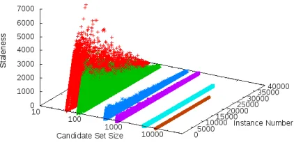
Figure 2: Staleness of theallowoldalgorithm over time for different candidate set sizes
4 Results
Two questions are pertinent regarding staleness: how much staleness does an algorithm introduce?
and how detrimental is that staleness? Forzerostale
andbatch, the first question was answered analyti-cally in a previous section. We proceed by
address-ing the answer empirically forallowoldandparallel
after which we examine the second question. Figure 2 shows the observed staleness of instances selected for annotation over time and for varying
candidate set sizes forallowold. As expected, small
candidate sets induce more staleness, in this case in very high amounts. Also, for any given candidate set size, staleness decreases over time (after the be-ginning stages), since the effective candidate set in-cludes an increasingly larger percentage of the data.
Since parallel is based on the same
allow-old-scores principle, it too could potentially see highly stale instances. However, we found the average
per-instance staleness ofparallelto be very low:1.10; it
was never greater than4in the range of data that we
were able to collect. This means that for our task and hardware, the amount of time that the oracle takes to annotate an instance is high enough to allow new models to retrain quickly and score a high percent-age of the data before the next instance is requested. We now examine effect that staleness has on
AL performance, starting withbatch. As we have
shown, higher batch sizes guarantee more staleness so we compare the performance of several batch
sizes (with a candidate set size of the full data) to
ze-rostaleandrandom. In order to tease out the effects that the staleness has on performance from the ef-fects that the batches have on wait time (an element of performance), we purposely ignore wait time.
The results are shown in Figure 3. Not surprisingly,
zerostaleis slightly superior to the batch methods, and all are superior to random selection.
Further-more,batch is not affected much by the amount of
staleness introduced by reasonable batch sizes: for
B <100the increase in cost of attaining 95%
accu-racy compared tozerostaleis 3% or less.
Recall that allowold introduces more staleness
thanbatch by maintaining old scores for each
in-stance. Figure 4 shows the effect of different
candidate set sizes on this approach while fixing batch size at 1 (wait time is excluded as before). Larger candidate set sizes have less staleness, so
not surprisingly performance approacheszerostale.
Smaller candidate set sizes, having more staleness, perform similarly to random during the early stages when the model is changing more drastically each instance. In these circumstances, scores produced from earlier models are not good approximations to the actual scores so allowing old scores is detrimen-tal. However, once models stabilize and old scores become better approximations, performance begins
to approach that ofzerostale.
Figure 6 compares the performance ofallowold
for varying batch sizes for a fixed candidate set size (5000; results are similiar for other settings). As before, performance suffers primarily in the early stages and for the same reasons. However, a batch excerbates the problem since multiple instances with poor scores are selected simultaneously. Neverthe-less, the performance appears to mostly recover once the scorers become more accurate. We note that batch sizes of 5 and 10 increase the cost of acheiving 95% accuracy by 3% and 10%, respectively,
com-pared to zerostale. The implications for parallel
are that stalness may not be detrimental, especially if batch sizes are small and candidate set sizes are large in the beginning stages of AL.
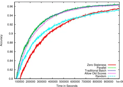
Figure 5 compares the effect of staleness on all
four algorithms when excluding wait time (B = 20,
N = 5000for the batch algorithms). After
achiev-ing around 85% accuracy, batch and parallel are
virtually indistinguishable fromzerostale, implying
that the staleness in these algorithms is mostly
ignor-able. Interestingly,allowoldcosts around 5% more
thanzerostale to acheive an accuracy of 95%. We attribute this to increased levels of staleness which
0.8 0.82 0.84 0.86 0.88 0.9 0.92 0.94 0.96
100000 200000 300000 400000 500000 600000 700000 800000 900000 1e+06
Accuracy
Time in Seconds
[image:7.612.323.532.75.224.2]Zero Staleness Batch size 5 Batch size 50 Batch size 500 Batch size 5000 Random
Figure 3: Effect of staleness due to batch size for
batch,N =∞
0.8 0.82 0.84 0.86 0.88 0.9 0.92 0.94 0.96
100000 200000 300000 400000 500000 600000 700000 800000 900000 1e+06
Accuracy
Time in Seconds
[image:7.612.87.296.75.225.2]Zero Staleness Candidate Set Size 5000 Candidate Set Size 500 Candidate Set Size 100 Candidate Set Size 50 Random
Figure 4: Effect of staleness due to candidate set size forallowold,B = 1
0.8 0.82 0.84 0.86 0.88 0.9 0.92 0.94 0.96
100000 200000 300000 400000 500000 600000 700000 800000 900000 1e+06
Accuracy
Time in Seconds
Zero Staleness Parallel Traditional Batch Allow Old Scores Random
Figure 5: Comparison of algorithms (not including wait time)
0.8 0.82 0.84 0.86 0.88 0.9 0.92 0.94 0.96
100000 200000 300000 400000 500000 600000 700000 800000 900000 1e+06
Accuracy
Time in Seconds
[image:7.612.86.294.289.438.2]Zero Staleness Batch Size 5 Batch Size 10 Batch Size 50 Batch Size 100 Batch Size 500 Random
Figure 6: Effect of staleness due to batch size for
allowold,N = 5000
0 50000 100000 150000 200000 250000
0 2000 4000 6000 8000 10000 12000
Instances Scored
Model Number
Figure 7: Effective candidate set size of parallel
over time
0.8 0.82 0.84 0.86 0.88 0.9 0.92 0.94 0.96
100000 200000 300000 400000 500000 600000 700000 800000 900000 1e+06
Accuracy
Time in Seconds
Zero Staleness Parallel Traditional Batch Allow Old Scores Random
[image:7.612.322.527.290.438.2] [image:7.612.324.531.505.652.2] [image:7.612.85.294.506.654.2]Since the amount of data parallel uses to train models and score instances depends on the amount of time instances take to annotate, the “effective” candidate set sizes and batch sizes over time is of in-terest. We found that the models were always trained after receiving exactly one instance, within the data we were able to collect. Figure 7 shows the number of instances scored by each successive scorer, which appears to be very large on average: over 75% of the time the scorer was able to score the entire dataset. For this task, the human annotation time is much greater than the amount of time it takes to train new models (at least, for the first 13,000 instances). The
net effect is that under these conditions,parallelis
parameterized similar tobatchwithB = 1andN
very high, i.e., approachingzerostale, and therefore
has very low staleness, yet does so without incurring the waiting cost.
Finally, we compare the performance of the four algorithms using the same settings as before, but in-clude wait time as part of the cost. The results are
in Figure 8. Importantly, parallel readily
outper-formszerostale, costing 40% less to reach 95%
ac-curacy. parallelalso appears to have a slight edge
overbatch, reducing the cost to acheive 95% accu-racy by a modest 2%; however, had the simulation continued, we we may have seen greater gains given the increasing training time that occurs later on. It is important to recognize in this comparison that the
purpose ofparallelis not necessarily to significantly
outperform a well-tuned batch algorithm. Instead, we aim to eliminate wait time without requiring pa-rameters, while hopefully maintaining performance. These results suggest that our approach successfully meets these criteria.
Taken as a whole, our results appear to indicate that the net effect of staleness is to make selection more random. Models trained on little data tend to produce scores that are not reflective of the actual utility of instances and essentially produce a ran-dom ranking of instances. As more data is collected, scores become more accurate and performance be-gins to improve relative to random selection. How-ever, stale scores are by definition produced using models trained with less data than is currently avail-able, hence more staleness leads to more random-like behavior. This explains why batch selection tends to perform well in practice for “reasonable”
batch sizes: the amount of staleness introduced by
batch (B−12 on average for a batch of sizeB)
intro-duces relatively little randomness, yet cuts the wait
time by approximately a factor ofB.
This also has implications for ourparallelmethod
of AL. If a given learning algorithm and scoring function outperform random selection when using
zerostaleand excluding wait time, then any added staleness should cause performance to more closely resemble random selection. However, once wait-ing time is accounted for, performance could
ac-tually degrade below that of random. Inparallel,
more expensive training and scoring algorithms are likely to introduce larger amounts of staleness, and would cause performance to approach random
selec-tion. However,parallelhas no wait time, and hence
our approach should always perform at least as well as random in these circumstances. In contrast, poor
choices of parameters inbatchcould perform worse
than random selection.
5 Conclusions and Future Work
Minimizing the amount of time an annotator must wait for the active learner to provide instances is an important concern for practical AL. We presented a method that can eliminate wait time by allowing in-stances to be selected on the basis of the most re-cently assigned score. We reduce the amount of staleness this introduces by allowing training and scoring to occur in parallel while the annotator is busy annotating. We found that on PTB data us-ing a MEMM and a ROI-based scorer that our pa-rameterless method performed slightly better than a hand-tuned traditional batch algorithm, without re-quiring any parameters. Our approach’s parallel na-ture, elimination of wait time, ability to dynamically adapt the batch size, lack of parameters, and avoid-ance of worse-than-random behavior, make it an
at-tractive alternative tobatchfor practical AL.
Since the performance of our approach depends on the relative time spent annotating, training, and scoring, we wish to apply our technique in future work to more complex problems and models that have differing ratios of time spent in these areas.
Fu-ture work could also draw on thecontinual
References
S. Arora, E. Nyberg, and C. P. Ros´e. 2009. Estimating annotation cost for active learning in a multi-annotator environment. InProceedings of the NAACL HLT 2009 Workshop on Active Learning for Natural Language Processing, pages 18–26.
S. P. Engelson and I. Dagan. 1996. Minimizing manual annotation cost in supervised training from corpora. In Proceedings of the 34th annual meeting on Associa-tion for ComputaAssocia-tional Linguistics, pages 319–326. R. A. Haertel, K. D. Seppi, E. K. Ringger, and J. L.
Car-roll. 2008. Return on investment for active learning. InNIPS Workshop on Cost Sensitive Learning. E. Horvitz. 2001. Principles and applications of
con-tinual computation. Artificial Intelligence Journal, 126:159–96.
M. P. Marcus, B. Santorini, and M. A. Marcinkiewicz. 1994. Building a large annotated corpus of en-glish: The penn treebank. Computational Linguistics, 19:313–330.
E. Ringger, M. Carmen, R. Haertel, K. Seppi, D. Lond-sale, P. McClanahan, J. Carroll, and N. Ellison. 2008. Assessing the costs of machine-assisted corpus anno-tation through a user study. InProc. of LREC. B. Settles, M. Craven, and L. Friedland. 2008. Active
learning with real annotation costs. InProceedings of the NIPS Workshop on Cost-Sensitive Learning, pages 1069–1078.