An explicit statistical model of learning lexical segmentation using
multiple cues
C¸a˘grı C¸¨oltekin
University of Groningen
John Nerbonne
University of Groningen
Abstract
This paper presents an unsupervised and incremental model of learning segmenta-tion that combines multiple cues whose use by children and adults were attested by experimental studies. The cues we exploit in this study are predictability statistics, phonotactics,lexical stressand partial lex-ical information. The performance of the model presented in this paper is competi-tive with the state-of-the-art segmentation models in the literature, while following the child language acquisition more faith-fully. Besides the performance improve-ments over the similar models in the liter-ature, the cues are combined in an explicit manner, allowing easier interpretation of what the model learns.
1 Introduction
Segmenting the continuous speech stream into lex-ical units is one of the challenges we face while lis-tening to other speakers. For competent language users, probably the biggest aid in identifying the word boundaries is the knowledge of the words. Not surprisingly, the models of adult word recog-nition depend heavily on a lexicon (see Dahan and Magnuson, 2006, for a recent review). The same can be observed in speech and language technol-ogy where all automatic speech recognition sys-tems make use of a comprehensive lexicon.
Even with a comprehensive lexicon and an error-free representation of the acoustic input, the problem is not trivial, since the input is often com-patible with multiple segmentations spanning the complete utterance. The problem, however, is even more difficult for a learner who starts with no lexicon. Fortunately, the lexicon is not the only aid for segmentation. Experimental research within last two decades has revealed an array of cues that are used by adults and children for lexi-cal segmentation. These cues include, but are not
limited to, lexical stress (Cutler and Butterfield, 1992; Jusczyk, Houston, et al., 1999), phonotac-tics (Jusczyk, Cutler, et al., 1993), predictability statistics (Saffran et al., 1996), allophonic differ-ences (Jusczyk, Hohne, et al., 1999), coarticula-tion(E. K. Johnson and Jusczyk, 2001), andvowel harmony (Suomi et al., 1997). The relative utility or dominance of these cues is a matter of current debate. However, it seems uncontroversial that none of these cues solves the segmentation prob-lem alone and, when available, they are used in conjunction.
Along with experimental research on segmen-tation, a large number of computational models have been proposed in the literature. The early studies typically made use of connectionist mod-els (e.g., Elman, 1990; Christiansen et al., 1998). Of these studies, Christiansen et al. (1998) is par-ticularly interesting for the present study since it incorporates most of the cues used in this study. Using a simple recurrent network (SRN, Elman, 1990), Christiansen et al. (1998) demonstrated the usefulness of lexical stress, predictability statistics (included implicitly in any SRN model), and utter-ance boundaries, and showed that combining the cues improves the performance. The connection-ist models have been instrumental in investigating a large number of cognitive phenomena. However, they have also been subject to the criticism that what a connectionist model learns is rather dif-ficult to interpret. Furthermore, the performance achieved using connectionist models is far lower than that is expected from humans.
Models that use explicit representations in com-bination with statistical procedures (e.g., Brent and Cartwright, 1996; Brent, 1999; Venkatara-man, 2001; Goldwater et al., 2009; M. Johnson and Goldwater, 2009) avoid both problems: these models perform better, and it is easier to reason about what they learn. Although these models were also instrumental in our understanding of the problem, they lack at least two aspects of
nectionist models that fit human processing better. First, even though we know that human segmen-tation is incremental and predictive, most of these models process their input either in a batch fash-ion, or they require the complete utterance to be presented before attempting to segment the input. Second, it is generally difficult to incorporate ar-bitrary cues into most of these models.
Models that use explicit representations with incremental models exist (e.g., Monaghan and Christiansen, 2010; Lignos, 2011), but are rather rare. Furthermore, the investigation of cues and cue combination in segmentation is also relatively scarce within the recent studies (exceptions in-clude the investigation of various suprevised mod-els by Jarosz and J. A. Johnson, 2013).
The present paper introduces a strictly incre-mental, unsupervised method for learning seg-mentation where the learning method and internal representations are explicitly defined. Crucially, we use a set of cues demonstrated to be used by humans in solving the segmentation problem. The simulations results that we present are based on the same child-directed speech input used by many other studies in the literature.
The rest of this article is organized as follows: in the next section, we present a method for com-bining cues. Section 3 describes the cues used in this study. The simulations are described and re-sults are presented in Section 4. A general discus-sion of the modeling framework and the simula-tion results are given in Secsimula-tion 5.
2 A cue combination method
We know that there is no single cue that always gives the correct answer in the lexical segmenta-tion task. We also know that humans combine multiple cues when available. In this section we define a method to segment a given utterance using multiple boundary indicators, or cues, and learn to segment better by estimating usefulness of each indicator. In essence, each indicator makes a de-cision on each potential boundary location. The method combines these indicators’ decisions to ar-rive at a hopefully more accurate decision. In ma-chine learning terms, we formulate a number of binary classifiers, and aim to get a better classi-fier using a combination of them. This problems is a relatively well-studied subject in the machine learning literature (e.g., Bishop, 2006, chapter 14). Here a simple and well-known method,
major-ity voting, will be used for combining multiple boundary indicators.
Majority voting is a common (and arguably ef-fective) method in everyday social and political life. As a result, it has been well studied, and known to work well especially if each voter’s de-cision is better than random on average, and votes are cast independently. In practice, even though the votes are almost never independent, majority voting is still an effective way of combining mul-tiple classifiers (see Narasimhamurthy, 2005, for a discussion of the effectiveness of the method).
The majority voting combines each vote equally. Even though this may be a virtue in the social and political context, it is a shortcoming for a computational procedure that incorporates infor-mation from multiple sources with varying useful-ness. We will use a simple augmentation of ma-jority voting to model, weighted majority voting (Littlestone and Warmuth, 1994), that weighs the utility of the information provided by each source. In weighted majority voting, the voters that make fewer errors get higher weights. In an un-supervised setting as ours, we do not know for certain when a voter makes an mistake. Instead, we take a voter’s decision to be correct if it agrees with the majority. Initially we set all the weights to 1, trusting all the voters equally. We adopt an incremental version of the algorithm, where we keep the count of ‘errors’ made by each voteri,
ei, which is incremented every time the voter dis-agrees with the majority. After every boundary de-cision, first, the error counts are updated for each voter. Then, the weight,wi, of each voter is up-dated using,
wi ←2
0.5−Nei
where N is the number of boundary decisions made so far, including the current one.
This update rule sets the weight of a voter that is half the time wrong (a voter that votes at ran-dom) to zero, eliminating the incompetent voters. If the votes of a voter are in accordance with the weighted majority decision almost all the time, the weight stays close to one.
3 Cues and boundary indicators
differ based on the source of information used and the way this information is turned into a quantita-tive measure. This section introduces all of these cues, and the boundary indicators that stem from quantification of these cues in different ways.
3.1 Predictability statistics
At least as early as Harris (1955), it was known that a simple property of natural language utter-ances can aid identifying the lexical units that form an utterance: predictability within the units is high, predictability between the units is low. However, until the influential study by Saffran, Aslin, and Newport (1996), the idea was not in-vestigated in developmental psycholinguistics as a possible source of information that children may use for segmentation. After Saffran et al. (1996) showed that 8-month-old infants make use of pre-dictability statistics to extract word-like units from an artificial language stream, a large number of studies confirmed that predictability based strate-gies are used by adults and children for learning different aspects of language (e.g., Thiessen and Saffran, 2003; Newport and Aslin, 2004; Graf Estes et al., 2007; Thompson and Newport, 2007; Perruchet and Desaulty, 2008).
To use in our cue combination system, we need to quantify the notion of predictability. In this study, we use two information theoretic measures of predictability (or surprise), to define a set of boundary indicators. The first one,pointwise mu-tual information(MI) is defined as
MI(l, r) =log2PP(l()l, rP()r)
wherelandr are strings of phonemes to the left and right of the possible boundary location. We define our second measure,boundary entropy(H) of a potential boundary after stringlas
H(l) = −X r∈A
P(r|l)log2(P(r|l))
where the sum ranges over all phonemes in the al-phabet,A.1
The use of both the MI and the H is moti-vated by the finding that combination multiple pre-dictability measures result in better segmentation 1The input to children is better represented by ‘segments’
or ‘phones’. However, since the data used in our simulations does not contain any phonetic variation, in this paper, we use the term phoneme when referring to the basic input unit.
(see C¸¨oltekin, 2011, p.101, for an analysis). Fur-thermore, for asymmetric measures, like entropy,
H(l)is clearly not the same asH(r). Motivated by the finding that children use ‘reverse predictabil-ity’ (Pelucchi et al., 2009), we also incorporate a reverse entropy measure in the present study.
In most studies in the literature, the context l
andrare single basic units (phonemes in our case). The different phoneme context sizes may capture regularities that exist because of different linguis-tic units. The relation between the phoneme con-text size and the linguistic units, of course, is not clear-cut. However, for example, we expect con-text size of one to capture the regularities between the phonemes, while context size of two or three to capture regularities between larger units, such as syllables.
The above parameters result in an array of in-dicators. However, none of the indicators we use have a natural threshold to decide whether a given position is a boundary or not. To get a boundary decision out of a single measure (MIor H), we adopt a method similar to a commonly used unsu-pervised method that decides for a boundary at the ‘peaks’ of unpredictability. A particular shortcom-ing of this strategy, however, is that it can never find both boundaries of a single-phoneme word, as there cannot be two peaks one after another. To remedy this, thepartial-peak strategy we employ here makes use of two sets of boundary indicators for each potential boundary: one posits a bound-aryafter an increase in H(or a decrease in MI) and the other posits a boundarybeforea decrease inH.
3.2 Utterance boundaries
An attractive aspect of the predictability-based segmentation is that it does not require any lexical knowledge in advance—unlike other cues noted in Section 1. However, certain aspects of phonotac-tics, such as the regularities found at the beginning and end of words, can be induced from the bound-aries already marked in the input without the need for a lexicon. As a result, clearly marked lexical unit boundaries may serve as another source of in-formation that can bootstrap the acquisition of lex-ical units.2
2There are a number of acoustic cues (e.g., pauses) that
All models of segmentation in the literature use utterance boundaries implicitly by assuming that the words cannot straddle utterance bound-aries. The explicit use of utterance boundaries to discover regularities about words is common in connectionist models (e.g., Aslin et al., 1996; Christiansen et al., 1998; Stoianov and Nerbonne, 2000). Similar use of utterance boundaries in non-connectionist models is rather rare. Three excep-tions to this are the models described by Brent (1996), Fleck (2008) and Monaghan and Chris-tiansen (2010). The method described in this sec-tion is similar to Fleck’s method, where the model estimates the probability of observing a boundary given its left and right context,P(b|l, r), whereb
represents boundary, and as before, l and r rep-resent left and right contexts, respectively. If this probability is greater than 0.5, the model inserts a boundary. Using utterance boundaries and the pauses, Fleck (2008) presents a batch algorithm with a few ad hoc corrections that estimates the probabilities P(b), P(l|b), P(r|b), P(l), P(r), and uses Bayesian inversion to estimateP(b|l, r).
In this work, instead of P(b|l, r), we estimate probabilities of utterance beginnings, P(ub|r), and probabilities of utterance ends, P(ub|l), where ub stands for utterance boundary. These probabilities can directly be estimated from the utterance edges in the input corpus, and can be used as cues for discovering initial or non-final boundaries. Similar to the predictability, us-ing different lengthlandrwe obtain a set of indi-cators forP(ub|r)andP(ub|l).
Unlike P(b|l, r), for P(ub|r) and P(ub|l) we do not have a straightforward threshold to make a boundary decision. Instead, we appeal to the familiar solution, and use ‘partial peaks’ in these values as boundary indications.
3.3 Lexical stress
Lexical stress is one of the cues for segmentation that is well supported by psycholinguistic research (e.g., Cutler and Butterfield, 1992; Jusczyk, Hous-ton, et al., 1999; Jusczyk, 1999). Lexical stress is used in many languages for marking the promi-nent syllable in a word. For languages that exhibit lexical stress, the prominent syllable will typically be in a particular position in the word, allowing discovery of the boundaries based on the position of stressed syllable.
Despite the prominence of stress as a cue for
segmentation, there are relatively few computa-tional studies that investigate use of stress. Chris-tiansen et al. (1998) incorporates stress as a cue in their connectionist cue combination system. Swingley (2005) provides a careful analysis of stress patterns of the bisyllabic words found by a discovery procedure on mutual information and frequency. Gambell and Yang (2006) present sur-prisingly good segmentation results with a rule-based learner whose main source of information is lexical stress. One of the major problems with the these studies, which has also been carried over to the present study, is the lack of corpora with re-alistic stress assignment (see Section 4.1).
Our stress-based strategy is similar to the strat-egy used for learning phonotactics described in Section 3.2. Instead of collecting statistics about phoneme n-grams, we collect statistics over stress assignments on phoneme n-grams. However, the probabilities are estimated over already known lexical units. Given stress patternslandr, we es-timate P(b|l) from endings of the known lexical units, andP(b|r)from the beginnings of the lexi-cal units. Again we use these quantities as indica-tors for variable lengthlandr. Using the partial-peak boundary decision strategy in combination with the weighted majority voting algorithm, as before, we define a set of boundary indicators and operationalize lexical stress as another cue for seg-mentation.
3.4 Lexicon
For adults, a comprehensive lexicon is probably the most useful cue for segmentation. We do not expect infants to have a lexicon at the begin-ning. However, as they build their lexicon, or ‘proto-lexicon’, they may put it in use for discov-ering novel lexical units. This is the main strat-egy behind the majority of state-of-the-art compu-tational models of segmentation (e.g., Brent, 1999; Venkataraman, 2001; Goldwater et al., 2009). The models that guess boundaries rarely build and use an explicit lexicon (exceptions include Monaghan and Christiansen, 2010).
loca-tion, we simply count the frequencies of already known words beginning or ending at the position in question. The second indicator is based on the number of times the phoneme sequences sur-rounding the boundary found at the beginnings or ends of the previously discovered words. The sec-ond indicator is essentially the same as the phono-tactics component discussed in Section 3.2, ex-cept that it is calculated using already known word types instead of utterance boundaries.
Similar to the other asymmetric indicators dis-cussed previously, we have two flavors for each in-dicator. One indicating the existence of words to the right of the boundary candidate (words begin-ning at the boundary), and the other indicating the existence of words the left of the boundary can-didate (word ending at the boundary). As with the other cues, these result in a set of indicators whose primary source of information is the potential lexi-cal units in the learner’s incomplete and noisy lex-icon.
4 Experiments 4.1 Data
We use a child-directed speech corpus from the CHILDES database (MacWhinney and Snow, 1985). It was collected by Bernstein Ratner (1987) and the original orthographic transcription of the corpus was converted to a phonemic transcription by Brent and Cartwright (1996). The same corpus has been used by many recent studies. Following the convention in the literature the corpus will be called theBR corpus.
For the results reported for segmentation strate-gies that make use of lexical stress, the BR corpus was marked for lexical stress semi-automatically following the procedure described by Christiansen et al. (1998) for annotating the Korman corpus (Korman, 1984). The stress assignment is done according to stress patterns in the MRC psycholin-guistic database. All single-syllable words are coded as having primary stress, and the words that were not found or did not have stress assignment in the MRC database were annotated manually.
4.2 Evaluation metrics
Two quantitative measures, precision (P), recall (R) and their harmonic meanF1-score(F-score, or
F, for short), have become the standard evaluation measures for computational simulations. Follow-ing recent studies in the literature we present
pre-cision recall and F-scores for boundaries (BP, BR, BF), word tokens (WP, WR, WF) and word types or lexicon (LP, LR, LF). Besides precision and recall, we also present two error measures, over-segmentation (Eo) and undersegmentation (Eu) er-rors, defined as Eo = FP/(FP+TN) andEu = FN/(FN+TP), where TP, FP, TN and FN are true positives, false positives, true negatives, and false negatives respectively.
In plain words, Eo is the number of the false boundaries inserted by the model divided by the total number of word internal positions in the corpus. Similarly, Eu is the ratio of boundaries missed to the total number of boundaries. Al-though these error measures are related to preci-sion and recall, they provide different, and some-times better, insights into the model’s behavior. 4.3 Reference models
In this paper, we compare the results obtained by the cue combination model with two baselines. The first baseline is a random model (RM) that assigns boundaries with the probability of bound-aries in the input corpus. The RM is more in-formed than a completely random classifier, but it has been customary (since Brent and Cartwright, 1996) in segmentation literature to set the bar a little bit higher. The second reference model is a lexicon-building model similar to many state-of-the-art models. The model described here, which we call LM, assigns probabilities to possible seg-mentations as described in Equations 1 and 2.
P(s) =Yn i=1
P(wi) (1)
P(w) =
(1−α)f(w) ifwis known
αQmi=1P(ai) ifwis unknown (2)
where s is a sequence of phonemes (e.g., an ut-terance or a corpus), wi is theith word in the se-quence,aiis theithsound in the word,f(w)is the relative frequency of the wordw,mis the number of known words, and0 ≤ α ≤ 1 is the only pa-rameter of the model. In all experiments reported in this paper, we will fixαat 0.5.
boundary word lexicon
model P R F P R F P R F
Brent (1999) 80.3 84.3 82.3 67.0 69.4 68.2 53.6 51.3 52.4 Venkataraman (2001) 81.7 82.5 82.1 68.1 68.6 68.3 54.5 57.0 55.7 Goldwater et al. (2009) 90.3 80.8 85.2 75.2 69.6 72.3 63.5 55.2 59.1 Blanchard et al. (2010) 81.4 82.5 81.9 65.8 66.4 66.1 57.2 55.4 56.3 RM 27.4 27.0 27.2 12.6 12.5 12.5 6.0 43.6 10.5 LM 84.1 82.7 83.4 72.0 71.2 71.6 50.6 61.0 55.3
Table 1: Performance scores of the reference mod-els LM and RM in comparison with some of the earlier scores reported in the literature. If there were multiple models reported in a study, the re-sult with the highest lexicon F-score is presented. All scores are obtained on the BR corpus.
Table 1 compares the performances of some re-cent models in the literature using the BR corpus with the two reference models. The LM performs similar to the state-of-the-art models presented in this table. Hence, to aid comparison of the mod-els proposed in this study with the others in the literature, we will (re)report the result of the two baseline models in the rest of this paper. Note that the scores presented in Table 1 can be mis-leading since the batch models have an advantage due to the way scores are calculated. The scores of the batch models are calculated at the end of training, while scores of the incremental models include initial (presumably bad) choices made be-fore enough exposure to the input. For example, the LM achieves boundary, word and lexicon F-scores of 89%, 81% and 74% respectively, towards the end of the BR corpus. These scores are higher than all of the scores presented in Table 1 (see Ta-ble 4 for details the way these scores are calcu-lated).
4.4 Experiments and results
This section reports results of a set of simulations using the modeling framework described so far. All experiments are run on the BR corpus. For all the results reported below, each cue is repre-sented by a set indicators as described in Section 3, multiple indicators for each phoneme n-gram of length one and three are used for left (l) and right (r) contexts, for all measures that are calculated over phoneme n-grams surrounding the potential boundary. The use of lexical information and lex-ical stress as standalone strategies are similar to the ‘lexicon-building’ strategy. The learner inserts complete utterances to the lexicon when the strat-egy cannot segment the utterance. As the learner starts to learn (from the edges of the sequences in
the lexicon) what the edges of words look like, it uses this information to segment later utterances in the input.3
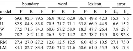
We first report the performance results of indi-vidual cues, namely, predictability (P),utterance boundaries(U),lexical information (W) and lexi-cal stress(S) in Table 2.
Using the predictability cue alone leads to a segmentation performance lower than but close to the state-of-the-art reference model LM. Although these results are not directly comparable to the earlier studies in the literature, the performance scores presented in Table 2 are the best scores pre-sented to date for models using the predictability cue alone. Graphs presented by Brent (1999) in-dicates about 50%–60% WP and WR and 20%– 30% LP for his baseline model utilizing mutual information on the BR corpus. Cohen et al. (2007) report 76% BP, and 75% BR on George Orwell’s 1984. Christiansen et al. (1998) report 37% WP and 40% WR with an SRN using phonotactics and utterance boundary cues on another child-directed speech corpus (Korman, 1984).
The model that learns from the utterance bound-aries seems to perform the best. The results are comparable, and in some cases better than the LM. Furthermore, the overall scores are also higher than the scores reported by Fleck (2008), where the boundary, word and lexical F-scores were 82.9%, 70.7% and 36.6%, respectively.
Although it is somewhat behind both pre-dictability and utterance boundary cues, the lexical information alone certainly performs better than random. The lower performance of this model in comparison to ‘U’ suggests that, at least in this set-ting, phonotactics learned from word tokens found at the utterance edges leads to a better perfor-mance compared to the phonotactics learned from the word types in the learner’s lexicon.
The experiment that takes only the stress cue into account yields the worst overall results. It seems, when the cue indicates a boundary, it is extremely precise. However, it is also very con-servative. This seems to be due to the fact that the model learns to segment at weak–strong tran-sitions, which is expected to be precise. However, since majority of the stress transitions are strong– strong, this covers rather a small portion of the boundaries.
3The source code of the application and the data used in
this study can be found athttps://bitbucket.org/
boundary word lexicon error
model P R F P R F P R F Eo Eu
P 69.6 92.5 79.5 56.9 70.2 62.9 36.7 49.8 42.3 15.3 7.5 U 82.9 84.8 83.8 70.5 71.7 71.1 33.8 66.9 44.9 6.6 15.2 W 77.5 71.3 74.3 60.6 57.2 58.9 18.3 47.7 26.4 7.8 28.7 S 78.2 8.2 14.8 26.5 9.7 14.2 8.2 38.7 13.5 0.9 92.8 RM 27.4 27.0 27.2 12.6 12.5 12.5 6.0 43.6 10.5 27.1 73.0 LM 84.1 82.7 83.4 72.0 71.2 71.6 50.6 61.0 55.3 5.9 17.3
Table 2: Results of simulations using individual cues: predictability (P), utterance boundaries (U), lexicon (W) and lexical stress (S). The rows la-beled LM and RM are scores of reference models repeated for ease of comparison.
boundary word lexicon error
model P R F P R F P R F Eo Eu
PU 82.6 90.7 86.5 72.4 77.4 74.8 42.8 65.3 51.7 7.2 9.3 PUW 83.7 91.2 87.3 74.1 78.8 76.4 43.9 67.7 53.3 6.7 8.8 PUWS 92.8 75.7 83.4 78.3 68.1 72.9 26.8 62.7 37.5 2.2 24.3 RM 27.4 27.0 27.2 12.6 12.5 12.5 6.0 43.6 10.5 27.1 73.0 LM 84.1 82.7 83.4 72.0 71.2 71.6 50.6 61.0 55.3 5.9 17.3
Table 3: Results of combination of strategies based on four cues: starting with predictability and utterance boundaries (PU), addition of lexi-con (PUW) and lexical stress (PUWS). The rows labeled LM and RM are scores of reference mod-els repeated for ease of comparison.
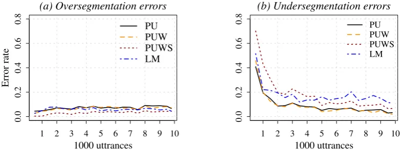
Table 3 presents combination of predictability and utterance boundaries, followed by lexical in-formation and stress. Here all indicators are bined in a flat, non-hierarchical manner. The com-bination of predictability and utterance bound-aries results in higher F-scores, and it results in more balanced und and ovsegmentation er-rors. The addition of the lexical information pro-vide a small but consistent improvement. How-ever, adding stress information seems to have an adverse effect. Despite the increased boundary and word precision, all other performance scores go down substantially when we add the stress cue. The scores in Table 3 are obtained over the com-plete corpus. As noted in Section 4.3, these scores do not reflect the ‘learned’ state of the models. Furthermore, we are interested in the progress of a learner as more input is provided. To demonstrate both,EoandEufor all combined models are plot-ted in Figure 1 for each 500 utterances.
An interesting observation that can be made in these graphs is that the models without the stress cue make fewer undersegmentation errors, with the cost of slightly higher oversegmentation. However, the strategy that combines all cues keeps
boundary word lexicon error
model P R F P R F P R F Eo Eu
[image:7.595.308.524.63.119.2]PU 85.6 96.7 90.8 78.7 86.0 82.2 71.8 75.9 73.8 6.6 3.3 PUW 83.3 97.2 89.7 75.6 84.5 79.8 69.8 75.5 72.5 7.9 2.8 PUWS 92.5 89.3 90.9 84.2 82.2 83.2 70.9 77.6 74.1 2.9 10.7
Table 4: The same results presented in Table 3, but measured for the last 290-utterances (last block in an incremental experiment with 500-utterance in-crements).
oversegmentation errors low throughout the learn-ing process, and towards the end, it makes fewer undersegmentation errors as well. This suggests that the model combining all cues, including the stress, may be doing better as it collects more evidence. To demonstrate this further, Table 4 presents the same results presented in Table 3, cal-culated on the last block of an experiment where performance scores were calculated after every 500 input utterances. Besides demonstrating the increase in performance scores when calculated at later stages of learning, the differences between tables 3 and 4 show clearly that despite the fact that it has a detrimental affect when scores are cal-culated over the complete corpus, the stress cue has a positive effect at the end of the learning pro-cess. This suggests that the combined model using stress cue learns slower and makes more mistakes at the beginning. However as evidence accumu-lates, it starts to be useful, and increases the over-all performance of the combined model.
5 General discussion
This paper introduced an unsupervised and in-cremental model of segmentation that focuses on combining multiple cues relevant to child lan-guage acquisition as attested by earlier studies in psycholinguistics. Unsupervised and incremen-tal models of segmentation that combine multiple cues are not new. There have been many models sharing these properties to some extent. In partic-ular, the model presented in this paper has many similarities with an earlier connectionist model of segmentation presented by Christiansen et al. (1998). However, unlike connectionist models, the model presented here uses accessible explicit rep-resentations, and an concrete learning procedure.
[image:7.595.72.291.64.149.2]0.0
0.2
0.4
0.6
0.8
(a) Oversegmentation errors
1000 uttrances
Error
rate
1 2 3 4 5 6 7 8 9 10 PU PUW PUWS LM
0.0
0.2
0.4
0.6
0.8
(b) Undersegmentation errors
1000 uttrances
[image:8.595.102.496.66.215.2]1 2 3 4 5 6 7 8 9 10 PU PUW PUWS LM
Figure 1: Progression of (a) over- and (b) under-segmentation errors of the combined strategies.
we get from these models are undeniably useful. However, these models typically provide explana-tions at Marr’s (1982) computational level. The modeling practice we follow is similar to these models in many ways, and can provide explana-tions for the same type of quesexplana-tions. However, it may also provide explanations at lower levels (e.g., Marr’s algorithmic level). This is not to claim that children learn exactly the way the model learns. However, the type of models presented in this paper follow human behavior more faithfully, and, at least in principle, more detailed predictions can be tested on these models. Naturally, rele-vance of the findings for human cognition will be increased as we constrain our models further in ac-cordance with what we know about the cognitive processes.
The first contribution of this study is the de-scription of a modeling framework that follows what we know about human segmentation process with high fidelity while keeping the benefits of a model with explicit representations and statistical learning methods.
Besides the performance scores that are com-petitive with the state-of-the-art models in the lit-erature, the simulations also provide some insights regarding the cues commonly studied in the psy-cholinguistics literature. Some of the findings con-firm the previous results. Indeed, it seems that combining multiple cues help. However, the prop-erties of the modeling framework presented in this paper allows us to make some other interesting ob-servations, for example, the effect of stress cue presented in Section 4.4.
When we look at the overall effect of the stress cue throughout the complete simulations, it seems stress degrades the performance. However, if we
take a look at the models’ performances at the end of the learning, we see that effect of the stress cue is actually positive. In other words, once ‘boot-strapped’ by the other cues, stress becomes a ful cue. Furthermore, the way the stress cue is use-ful for the model is also in line with the findings in the literature where stress is commonly found to be a dominant cue (Jusczyk, Cutler, et al., 1993; Thiessen and Saffran, 2003). Given the findings here that stress is rather a precise cue (despite its low recall), it is understandable why it dominates the boundary decisions when available.
References
Richard N. Aslin, Julide Z. Woodward, Nicholas P. LaMen-dola, and Thomas G. Bever (1996). “Models of Word Seg-mentation in Fluent Maternal Speech to Infants”. In: Sig-nal to Syntax: Bootstrapping From Speech to Grammar in Early Acquisition. Ed. by James L. Morgan and Katherine Demuth. Lawrence Erlbaum Associates. Chap. 8, pp. 117– 134.
Nan Bernstein Ratner (1987). “The phonology of parent-child speech”. In: Children’s language. Ed. by K. Nel-son and A. van Kleeck. Vol. 6. Hillsdale, NJ: Erlbaum, pp. 159–174.
Christopher M. Bishop (2006).Pattern Recognition and Ma-chine Learning. Springer.
Daniel Blanchard, Jeffrey Heinz, and Roberta Golinkoff (2010). “Modeling the contribution of phonotactic cues to the problem of word segmentation”. In:Journal of Child Language37.Special Issue 03, pp. 487–511.
Michael R. Brent (1996). “Advances in the computational study of language acquisition”. In: Cognition 61 (1-2), pp. 1–38.
Michael R. Brent (1999). “An Efficient, Probabilistically Sound Algorithm for Segmentation and Word Discovery”. In:Machine Learning34.1-3, pp. 71–105.
Michael R. Brent and Timothy A. Cartwright (1996). “Distri-butional regularity and phonotactic constraints are useful for segmentation”. In:Cognition61 (1-2), pp. 93–125. Morten H. Christiansen, Joseph Allen, and Mark S.
Seiden-berg (1998). “Learning to Segment Speech Using Multiple Cues: A Connectionist Model”. In:Language and Cogni-tive Processes13.2, pp. 221–268.
Paul Cohen, Niall Adams, and Brent Heeringa (2007). “Vot-ing experts: An unsupervised algorithm for segment“Vot-ing se-quences”. In:Intelligent Data Analysis11.6, pp. 607–625. C¸a˘grı C¸¨oltekin (2011). “Catching Words in a Stream of Speech: Computational simulations of segmenting tran-scribed child-directed speech”. PhD thesis. University of Groningen.
Anne Cutler and Sally Butterfield (1992). “Rhythmic cues to speech segmentation: Evidence from juncture mispercep-tion”. In:Journal of Memory and Language31.2, pp. 218– 236.
Delphine Dahan and James S. Magnuson (2006). “Spoken Word Recognition”. In: Handbook of Psycholinguistics. 2nd. Elsevier. Chap. 8, pp. 249–283.
Jeffrey L. Elman (1990). “Finding Structure in Time”. In:
Cognitive Science14, pp. 179–211.
Margaret M. Fleck (2008). “Lexicalized phonotactic word segmentation”. In:Proceedings of the Annual Meeting of the Association of Computational Linguistics (ACL-08), pp. 130–138.
Timothy Gambell and Charles Yang (2006).Word segmenta-tion: Quick but not dirty. Unpublished manuscript. Sharon Goldwater, Thomas L. Griffiths, and Mark Johnson
(2009). “A Bayesian framework for word segmentation: Exploring the effects of context”. In:Cognition 112 (1), pp. 21–54.
Katharine Graf Estes, Julia L. Evans, Martha W. Alibali, and Jenny R. Saffran (2007). “Can Infants Map Meaning to Newly Segmented Words? Statistical Segmentation and Word Learning”. In:Psychological Science18.3, pp. 254– 260.
Zellig S. Harris (1955). “From Phoneme to Morpheme”. In:
Language31.2, pp. 190–222.
Gaja Jarosz and J. Alex Johnson (2013). “The Richness of Distributional Cues to Word Boundaries in Speech to Young Children”. In: Language Learning and Develop-ment9.2, pp. 175–210.
Elizabeth K. Johnson and Peter W. Jusczyk (2001). “Word Segmentation by 8-Month-Olds: When Speech Cues Count More Than Statistics”. In:Journal of Memory and Language44.4, pp. 548–567.
Mark Johnson and Sharon Goldwater (2009). “Improving nonparameteric Bayesian inference: experiments on unsu-pervised word segmentation with adaptor grammars”. In:
Proceedings of Human Language Technologies: The 2009 Annual Conference of the North American Chapter of the Association for Computational Linguistics, pp. 317–325. Peter W. Jusczyk (1999). “How infants begin to extract
words from speech”. In:Trends in Cognitive Sciences3.9, pp. 323–328.
Peter W. Jusczyk, Anne Cutler, and Nancy J. Redanz (1993). “Infants’ preference for the predominant stress patterns of English words”. In: Child Development 64.3, pp. 675– 687.
Peter W. Jusczyk, Elizabeth A. Hohne, and Angela Bauman (1999). “Infants’ sensitivity to allophonic cues for word segmentation”. In: Perception and Psychophysics 61.8, pp. 1465–1476.
Peter W. Jusczyk, Derek M. Houston, and Mary New-some (1999). “The Beginnings of Word Segmentation in English-Learning Infants”. In:Cognitive Psychology 39, pp. 159–207.
Myron Korman (1984). “Adaptive aspects of maternal vocal-izations in differing contexts at ten weeks”. In:First Lan-guage5, pp. 44–45.
Constantine Lignos (2011). “Modeling infant word segmen-tation”. In: Proceedings of the Fifteenth Conference on Computational Natural Language Learning, pp. 29–38. Nick Littlestone and Manfred K. Warmuth (1994). “The
Weighted Majority Algorithm”. In:Information and Com-putation108.2, pp. 212–261.
Brian MacWhinney and Catherine Snow (1985). “The child language data exchange system”. In:Journal of Child Lan-guage12.2, pp. 271–269.
David Marr (1982).Vision: A Computational Investigation into the Human Representation and Processing of Visual Information. New York: Freeman.
Padraic Monaghan and Morten H. Christiansen (2010). “Words in puddles of sound: modelling psycholinguistic effects in speech segmentation”. In:Journal of Child Lan-guage37.Special Issue 03, pp. 545–564.
Anand Narasimhamurthy (2005). “Theoretical Bounds of Majority Voting Performance for a Binary Classification Problem”. In:IEEE Trans. Pattern Anal. Mach. Intell.27 (12), pp. 1988–1995.
Elissa L. Newport and Richard N. Aslin (2004). “Learning at a distance: I. Statistical learning of non-adjacent depen-dencies”. In:Cognitive Psychology48.2, pp. 127–162. Bruna Pelucchi, Jessica F. Hay, and Jenny R. Saffran (2009).
“Learning in reverse: Eight-month-old infants track back-ward transitional probabilities”. In: Cognition 113.2, pp. 244–247.
Pierre Perruchet and St´ephane Desaulty (2008). “A role for backward transitional probabilities in word segmenta-tion?” In:Memory and Cognition36.7, pp. 1299–1305. Jenny R. Saffran, Richard N. Aslin, and Elissa L. Newport
(1996). “Statistical learning by 8-month old infants”. In:
Science274.5294, pp. 1926–1928.
Ivelin Stoianov and John Nerbonne (2000). “Exploring Phonotactics with Simple Recurrent Networks”. In: Pro-ceedings of Computational Linguistics in the Netherlands 1999. Ed. by Frank van Eynde, Ineke Schuurman, and Ness Schelkens, pp. 51–67.
Daniel Swingley (2005). “Statistical clustering and the con-tents of the infant vocabulary”. In:Cognitive Psychology
50.1, pp. 86–132.
Erik D. Thiessen and Jenny R. Saffran (2003). “When Cues Collide: Use of Stress and Statistical Cues to Word Bound-aries by 7- to 9-Month-Old Infants,” in: Developmental Psychology39.4, pp. 706–716.
Susan P. Thompson and Elissa L. Newport (2007). “Statisti-cal Learning of Syntax: The Role of Transitional Probabil-ity”. In:Language Learning and Development3.1, pp. 1– 42.