Munich Personal RePEc Archive
Global Variance Risk Premium and
Forex Return Predictability
Aloosh, Arash
BI Norwegian Business School
19 November 2014
Global Variance Risk Premium and Forex Return
Predictability
(Job Market Paper)
Arash Aloosh
∗November 19, 2014
Abstract
In a long-run risk model with stochastic volatility and complete markets, I express expected forex returns as a function of consumption growth variances and equity variance risk premiums (VRPs)—the difference between the risk-neutral and statistical expectations of market return variation. This provides a motivation for using the forward-looking information available in stock market volatility indices to predict forex returns. Empirically, I find that equity VRPs predict forex returns at a one-month horizon, both in-sample and out-of-sample. Moreover, compared to two major currency carry predictors, global VRP has more predictive power for currency carry trade returns, bilateral forex returns, and excess equity return dif-ferentials.
Keywords: Global Variance Risk Premium; Excess Foreign Exchange (Forex) Return; Complete Markets; Predictability.
∗Department of Financial Economics at BI Norwegian Business School; arash.aloosh@bi.no; The
1 Introduction
Nominal exchange rate movements are difficult to predict out-of-sample (Meese and Rogoff (1983) and Rogoff (2009)), particularly at short horizons (Chinn and Meese (1995) and Rogoff and Stavrakeva (2008)). However, there is no economic reason that nominal exchange rate movements should not have some predictability. Indeed, from a theoretical perspective, equity market information should help to predict forex returns in complete markets (for example see Stulz (1981a and 1981b)). This provides a motivation for studying the predictive power of return predictors across markets; for example, an equity predictor such as the dividend yield has in-sample predictive power for forex returns, and a forex predictor such as the forward premium has in-sample predictive power for equity returns (Bekaert and Hodrick (1992)). This paper studies whether forward-looking information available in stock market volatility indices helps to predict forex returns, in-sample and out-of-in-sample.
A parsimonious intuition for the predictive power of stock market volatility indices is as follows: a volatility index measures the expectation of stock market volatility over the next period. When a stock market volatility index is significantly higher than the realized stock market volatility, it means that investors expect higher uncertainty over the next period. As a result, domestic agents require higher returns on their domestic and foreign investments. Therefore, domestic stock prices adjust (decrease) to compensate domestic agents to invest in the domestic stock market, and nominal spot exchange-rates adjust (decrease) to compensate them to invest abroad. However, nominal exchange-rates should adjust somehow to compensate both domestic and foreign investors, thus when the expected uncertainty of domestic agents increases (decreases) relative to that of foreign agents, the nominal spot exchange-rates decrease (increase), which predict higher (lower) nominal spot exchange-rates in the future.
This paper finds empirical evidence that the excess foreign exchange (forex) returns are predictable by equity VRPs at the one-month horizon, both in-sample and out-of-sample. This is the main contribution of the paper. In particular, the paper finds that local and global equity VRPs predicts forex returns of major forex returns, namely the pound, the yen, and the euro against the U.S. dollar, with an adjusted R-square of up to 17%. The local equity VRP is measured by the difference between the squared volatility index (e.g., V IX2) and the realized variance of the respective stock index (e.g.,S&P500)
in a country.1 For example, when the local equity VRP increases by one percent in the
1This measure of local VRP is a forward-looking measure of expected stock market volatility risk and
US (in the UK), the expected pound-dollar forex return increases (decreases) by around 5% (3%), and when the global equity VRP increases by one percent, the expected pound-dollar forex return increases by around 3%. The in-sample and out-of-sample R-squares of equity VRP predictions vary up to 17%.
Moreover, I run a ”horse race” among three currency predictors—the commodity and the currency volatility factors of Bakshi and Panayotov (2013) and the global VRP—to predict currency carry trade returns, bilateral forex returns, and cross-country equity return differentials. I find first that the global VRP has significantly higher predictive power for the carry trade returns, the bilateral forex returns, and the cross-country equity return differentials. Secondly, I find that the global VRP—which is primarily a equity predictor—has similar predictive power for a bilateral forex returns and the respective cross-country equity return differential, and that the commodity and the currency volatil-ity factors—which are primarily currency predictors—also have similar predictive power for a bilateral forex return and the respective cross-country equity return differential. Documenting the predictive power of these predictors across forex and equity markets is another novel empirical feature of this paper.
To formalize the link between forex returns and equity variance risk premiums, I merge the general currency-pricing model of Bekaert (1996) and Backus, Foresi, and Telmer (2001) and the long-run risk with stochastic volatility model of Bollerslev, Tauchen, and Zhou (2009). As discussed by Bekaert (1996) and Backus et al. (2001), among others, with complete markets the log forex return is equal to the difference between the log of the stochastic discount factor (SDF) variance in the two countries.2 Therefore, I
derive the model-implied log SDF variance in a two-country long-run risk model, which is constructed by merging the aforementioned models for currency pricing and long-run risk. I find that it has two components: consumption growth variance and the variance risk premium. By substituting them in the model of Bekaert (1996) and Backus et al.
(2001), I find that the expected forex returns are a function of the consumption growth variances and equity VRPs. The theoretical relation between expected forex returns and the equity VRPs (the global and country-specific VRPs) is a novel result in this paper.
A theoretical explanation for the predictive power of the global and country-specific
isolate the factor associated with the volatility of consumption growth volatility.
2
VRPs is that they measure agents’ perceptions of aggregate uncertainty and major shocks to the economic state variables globally and domestically, respectively. In theory, time-varying uncertainty in an economy with agents who have a risk aversion greater than one and Epstein–Zin preferences for early resolution of the uncertainty generate time-varying VRPs (Drechsler and Yaron (2011); Bollerslev et al. (2014)). Moreover, heterogeneity in exposure to the global VRP, specifically the high exposure of the low-interest-rate countries and the low exposure of the high-interest-rate countries, generates a currency risk premium. In a complete market with complete home bias and under lognormality, the domestic agent with a higher exposure to the global VRP is exposed to more uncertainty in periods where global uncertainty is high. As a result, the equilibrium domestic currency appreciates (or the foreign currency depreciates) to compensate the domestic agent for investing in the foreign bonds (as the domestic agent requires higher returns). At the same time, the higher uncertainty pushes down the domestic interest rate. The lower spot exchange rate and the lower domestic interest rate predict a higher excess forex return.
To support the common predictive power of the global equity VRP across markets (and also to motivate the ”horse race” among the predictors of different financial assets), I derive the model-implied cross-country equity return differentials and model-implied interest rate in complete markets. I find that they are driven by consumption growth variances and equity VRPs (global and local equity VRPs) as well. This commonality in driving factors supports the global risk interpretation of the global VRP. In addi-tion, it provides an explanation for the high degree of contemporaneous comovements between cross-country equity premium differentials and forex returns documented in Hau and Rey (2006), the predictive power of dividend yield—an equity return predictor—for forex returns documented in Bekaert and Hodrick (1992), the predictive power of forward premium—a forex return predictor—for excess equity returns documented in Bekaert and Hodrick (1992). It also explain the predictive power of global equity VRP for currency returns and the predictive power currency predictors for equity-return differentials doc-umented in this paper.
(2013) introduce an inflation-augmented two-country long-run risk model with stochas-tic volatility where the risk premiums are driven by the volatilities of expected growth and expected inflation. In particular, they use average forecasts of one-year-ahead real GDP growth and inflation from the Survey of Professional Forecasters to estimate the conditional volatilities of expected growth and inflation. This paper augments the con-sumption process in a two-country long-run risk model with stochastic volatility, where the risk premiums are driven by variance risk.
In addition, Bansal and Shaliastovich (2007 and 2013) and Colacito and Croce (2011) assume complete markets where agents have the same preference specifications across countries. I also assume complete markets, but consider the case where agents have different preference specifications across countries.3 Moreover, I assume that consumption
in each country is driven by a global factor and an orthogonal country-specific factor. As the agents have different exposures to the global factor in the economy, I show that expected forex returns are a function of the global and country-specific components of both consumption growth variance and VRP. On the one hand, consumption growth variance has little or no predictive power for bilateral forex returns, and adding it to the predicting regressions does not change the predictive power of the global and country-specific VRPs. On the other hand, this model simplifies to the model of Bansal and Shaliastovich (2007) when agents have the same preferences and VRPs are equal across countries.
There is a growing empirical literature studying the predictive power of VRPs for different financial assets. Bollerslev et al. (2009), Drechsler and Yaron (2011), and Bekaert and Hoerova (2014) find a strong relation between VRPs and excess equity returns. Bollerslev et al. (2014) find that the global VRP is even a better predictor for local excess equity returns than the local VRPs. Zhou (2009) and Mueller et al. (2011) find a strong relation between the VRP and excess bond returns in the United States. In particular, there is an emerging literature investigating the predictive power of equity and currency VRPs for forex returns.4 Della Corte, Ramadorai, and Sarno (2014) study
the cross-sectional link between currency VRPs and currency returns. Londono and Zhou (2012) investigate the time-series predictive power of currency VRPs for forex returns, and they show that currency VRP is related to currency-specific risks and that adding currency VRPs to the U.S. equity VRP increases the predictability of forex returns. Although others focus on currency VRPs, I examine equity VRPs instead, which has
3Backus, Gavazzoni, Telmer, and Zin (2010) also assume asymmetric economies, where central banks
react differently (more or less) to the exchange rates. There are several empirical and theoretical papers that support such asymmetries, for example, Benigno (2004), Eichenbaum and Evans (1995), and Engel and West (2006).
4The currency VRP is defined as the risk-neutral and statistical expectations of the future currency
some advantages from a perspective of complete markets. To the best of my knowledge, the current paper is the first to study and document the predictive power of equity VRPs (and particularly the global equity VRP) for forex returns.
Finally, I perform a number of robustness checks. I find that the global and the country-specific VRPs have predictive power when using Seemingly Unrelated Regressions (SURs), when including global and country-specific consumption growth variances in the regressions, and more importantly when excluding the 2008 crisis months from the sample. Moreover, the global VRP and the U.S.-specific VRP are strong predictors of forex returns for the majority of the other 18 currencies with respect to the U.S. dollar even when their local VRPs are unavailable.
The rest of the paper is organized as follows. Section 2 presents a two-country model in complete markets with stochastic volatilities. I describe the data in section 3 and the empirical findings and the robustness checks in section 4. I compare the predictive power of the global VRP with two currency return predictors across equity and forex markets in section 5. Then, I evaluate the out-of-sample performance of the equity VRPs in section 6. Section 7 concludes.
2 Complete Markets with Stochastic Volatilities: A Two-Country
Model
2.1 Preferences
I assume that the representative agents in the economy have the following Epstein and Zin (1989) preferences:
Ut=
n
(1−δ)C1−
γ θ
t +δEt
U1−γ t+1
1θo θ
1−γ
(1)
where Ct is aggregate consumption at time t, δ denotes the time discount factor, γ ≥ 0 refers to the coefficient of risk aversion, ψ ≥ 0 is the intertemporal elasticity of substi-tution, and θ ≡ (1−γ)
(1−1/ψ). As shown by Epstein and Zin (1991), these preferences imply that the logarithm of the stochastic discount factor (SDF), mt+1, depends on both the
log aggregate consumption growth rate, gt+1, and the return from time t to t+1 on the
asset that delivers aggregate consumption, rt+1:
mt+1 =θlogδ−
θ
2.2 The Consumption Process
The consumption asset return is not observable. However, to express the SDF in Equation 2 in terms of state variables and aggregate shocks, I specify consumption ex-ogenously. This is similar to Bansal and Yaron (2004), Bansal and Shaliastovich (2007 and 2013), and Colacito and Croce (2011) and this assumption helps to solve for the equilibrium real value of financial assets. A complete home bias—both representative agents are willing to consume only the goods with which they are endowed—suppresses the motivation to trade endowments across borders in this economy. Moreover, to incor-porate stochastic volatility in the equilibrium asset prices, as in Bollerslev et al. (2009), I assume that the geometric growth rate of consumption, gt+1 = log(ct+1/ct), and the
consumption growth volatility, σg,t+1, have the following joint process
gt+1 =µg+σg,tzg,t+1, (3)
σg,t2 +1 =aσ+ρσσg,t2 +√qtzσ,t+1, (4)
qt+1 =aq+ρqqt+ϕq√qtzq,t+1, (5)
where µg > 0 represents the constant mean growth rate, σ2g,t denotes the time-varying variance in consumption growth with volatility-of-volatility in the consumption growth process, qt. The parameters satisfy aσ > 0, aq > 0, |ρσ| < 1, |ρq| < 1, and ϕq > 0; and
{zg,t}, {zσ,t}, {zq,t} are iid Normal(0,1) processes jointly independent from each other.5
2.3 SDF in A Single Country
The return on the exogenous consumption assets, using standard Campbell and Shiller (1988) log-linearization, is given by6
rt+1=−logδ+
µg
ψ −
(1−γ)2
(2θ) σ
2
g,t+(κ1ρq−1)Aqqt+σg,tzg,t+1+κ1√qt[Aσzσ,t+1+Aqϕqzq,t+1],
(6) where
5Please see the details of the global and country-specific consumption processes behind Equation 22
in the Appendix B.
6
Aσ =
(1−γ)2
2θ(1−κ1ρσ)
, Aq =
1−κ1ρq−
q
(1−κ1ρq)2−θ2κ41ϕ2qA2σ
θκ2 1ϕ2q
. (7)
As κ1 > 0, γ > 1, and ψ > 1, both impact coefficients associated with the volatility
state variables are negative, i.e., Aσ < 0 and Aq < 0. Therefore, the return on the consumption asset increases by both higher short-term consumption growth volatility
σg,t, or higher consumption growth vol-of-volqt to compensate representative agents who bear these risks.
To find the equilibrium market prices of consumption and volatility risks, we need to express the conditional mean of the log SDF and its innovations as a function of the state variables:
mt+1 =logδ−
µg
ψ + (θ−1−
θ
ψ)σg,tzg,t+1−
(θ−1)(1−γ)2
(2θ) σ
2
g,t
+(θ−1)(κ1ρq−1)Aqqt+ (θ−1)κ1√qt[Aσzσ,t+1+Aqϕqzq,t+1], (8)
mt+1−Et[mt+1] =−γσg,tzg,t+1−(1−θ)κ1√qt[Aσzσ,t+1+Aqϕqzq,t+1]. (9)
The equilibrium market prices of risks are equal to
λc =γ, λq = (1−θ)κ1[Aσzσ,t+1+Aqϕqzq,t+1]. (10)
The price of consumption growth risks, λc, is equal to the risk-aversion coefficient
γ, which is exactly equal to the price of short-run consumption risks in Bansal and Shaliastovich (2013) and Colacito and Croce (2011). When agents have preferences for early resolution of uncertainty (γ > 1
ψ or 1> θ), the market price of consumption growth volatility risk, λq, is positive.
realized stock market variance—to estimate the consumption growth volatility risk. Furthermore, I construct a global measure of consumption growth volatility risk fac-tors by averaging local VRPs. This is because in my model, the preference parameters are not equal across countries, which is in contrast to the preference specifications in Bansal and Shaliastovich (2013) and Colacito and Croce (2011). In addition, I assume that con-sumption in different countries has a common factor. These two ascon-sumptions help me to explore a common factor to which the representative agents are heterogeneously exposed. I use a set of local VRPs to construct a global VRP, which mimics the common factor. In other words, I use information available in the set of local equity VRPs to predict their bilateral currency returns. The conditional mean of the log SDF and its innovations, as a function of such global state variables, is presented in the appendix.
2.4 SDFs in Two Countries: Currency Pricing
As noted by Bekaert (1996) and Backus, Foresi, and Telmer (2001), among others, in complete markets with lognormal marginal utilities, the law of one price implies that the relative value of the marginal utility of foreign currency versus domestic currency determines the associated exchange rate. In other words, the logarithm of exchange rate changes is equal to the difference between the logarithms of stochastic discount factors in the two countries;
sij,t+1−sij,t=mtj+1−mit+1, (11)
where the preference specifications in domestic country i are analogous in the foreign country j. mi
t+1 is the log SDF in the domestic country i, m
j
t+1 is the log SDF in the
foreign country j, and sij,t is the domestic spot price of one unit of foreign currency. A one-period forex return is given by:
rxf xij,t+1 =sij,t+1−sij,t−rfit+rf j
t. (12)
The variablerft is the risk-free rate at time t. Lustig et al. (2011) measurerx as the log excess return on buying a foreign currency in the forward market and then selling it in the spot market in the next period.
will be a function of the difference of the variance of log SDFs in the two countries:
E[rxf xij,t+1] =E[sij,t+1−sij,t−rfit+rf j
t] (13)
E[rxf xij,t+1] =E[mjt+1−mit+1−rfit+rfjt] (14)
E[ij, rxf xt+1] = 1 2var[m
i t+1]−
1 2var[m
j
t+1]. (15)
Therefore, a shock that increases the variance of log SDF in the domestic country relative to that in the foreign country increases the expected excess foreign exchange return.7
Under the aforementioned assumptions, I calculate the variance of log SDFs in country i and j as a function of state variables as follows (see the details of derivations in Appendix A),
var[mit+1] =γi2[σ2i,g,t] + (θi−1)2κi,12(Aσi
2+A
i,q2ϕi,q2)[qi,t], (16)
var[mjt+1] =γj2[σj,g,t2 ] + (θj−1)2κj,12(Aσj
2+A
j,q2ϕj,q2)[qj,t]. (17) By substituting Equations 16 and 17 in Equation 15,
E[rxf xt+1] = 1 2 γ
2
j[σj,g,t2 ]−γi2[σi,g,t2 ]
−12 (θj−1)2κj,12(Aσj
2+A
j,q2ϕj,q2)[qj,t]−(θi−1)2κi,12(Aσi
2+A
i,q2ϕi,q2)[qi,t]
. (18)
Equations 16 and 17 show that the variance of log SDF has two components: the con-sumption growth variance and the concon-sumption growth volatility-of-volatility. A positive shock to either of the volatilities increases the variance of log SDF. In other words, when the domestic consumption growth volatility relatively increases, the equilibrium domestic price of foreign currency drops immediately or the foreign currency depreciates. Thus, relative to the new equilibrium price today, we expect the foreign currency to appreciate tomorrow, as shown in Equation 18. This is similar to the model implications for short-run consumption volatility in Bansal and Shaliastovich (2007 and 2013) and Colacito and
7
Note that the variance of spot exchange rate changes is var[sij,t+1−sij,t] = var[m j t+1−m
i t+1].
Hence,
var[sij,t+1−sij,t] =var[m j
t+1] +var[m
i
t+1]−2cov[m
j t+1, m
i t+1].
In other words, the variance of the spot rate changes is a function of”sum”of variance of log SDFs in two countries and their covariance, while the expected forex returns are a function of just the”difference”
Croce (2011).
Equation 18 also suggests that when the domestic consumption growth volatility-of-volatility relatively increases, the equilibrium domestic price of foreign currency drops and the expected forex return increases. This is in line with the expected long-run con-sumption growth risk in Bansal and Shaliastovich (2013) and Colacito and Croce (2011). However, I use the expected consumption growth volatility-of volatility instead of the expected long-run consumption growth risk.
2.5 Variance Risk Premiums
Bollerslev et al. (2009) show that the equity VRP, which is the difference between the risk-neutral and realized variances of stock market returns (EtQ(σ2
r,t+1)−Et(σr,t2 +1)),
proxies the factor associated with the consumption growth volatility-of volatility, qt;
(θ−1)κ1(Aσ +Aqκ12(Aσ2+Aq2ϕq2)ϕq2)[qt]≃[V RPt]. (19) By substituting this statement in Equation 16, the variance of log SDF is a function of the consumption growth variance and VRP,
var[mt+1] =γ2[σg,t2 ] +λ[V RPt], (20)
whereλ= (θ−1)2κ12(Aσ2+A
q2ϕq2)
(θ−1)κ1(Aσ+Aqκ12(Aσ2+Aq2ϕq2)ϕq2) >0.
8 Finally, if we substitute Equation 20 into
Equation 15, we get:
E[rxf xij,t+1] = 1 2{γ
2
i[σi,g,t2 ] +λi[V RPi,t]} − 1 2{γ
2
j[σj,g,t2 ] +λj[V RPj,t]}
E[rxf xij,t+1] = 1 2{γ
2
i[σi,g,t2 ]−γj2[σj,g,t2 ]}+ 1
2{λi[V RPi,t]−λj[V RPj,t]} (21)
whererxf xij,t+1is the country i vis-`a-vis country j forex return (i=domestic and j=foreign),
σ2
i,g,t is consumption growth volatility in country i, andV RPi,t is the local VRP in coun-try i. Equation 21 says that the forex return has two components. The first component is a function of the difference in consumption growth variances across countries, and the second component is a function of the difference in VRPs across countries.9
8Having
γ >1 andψ >1 impliesθ <0. In addition, impact coefficients associated with both of the volatility state variables are negative (Aσ<0 andAq <0) andκ1>0; these imply that λ >0.
9Several studies find the consumption growth variance differential is not a strong predictor of excess
2.6 Decomposing Global and Country-Specific Components
Equation 21 is derived in an economy without a common factor. If we assume an econ-omy in which consumption in each country is driven by a global factor and an orthogonal country-specific factor, we can decompose the global and the country-specific components of both the consumption growth volatility and the VRP. Then, we can express the ex-pected forex return as a function of the global and the country-specific components (see Appendix B for the decompositions and the derivations):
E[rxf xij,t+1] = 1 2(γ
gl2
i τgi
2
−γjgl2τgj
2
)[σg,tgl2] + 1 2γ
si2
[σg,tsi2]− 1 2γ
sj2
[σsjg,t2]
+1 2(λ
gl i τri
2
−λglj τrj2)[V RPtgl] +1 2λ
si[V RPsi t ]−
1 2λ
sj[V RPsj
t ]. (22)
σg,tgl is the global consumption growth volatility, σg,tsi is country i-specific consumption growth volatility,V RPtgl is the global VRP,V RPtsiis country i-specific VRP,τgiis country i exposure to global consumption growth volatility, and τi
r is country i exposure to global consumption asset returns.
Equations 21 and 22 provide a motivation for the empirical predictability tests con-ducted in section 4.
3 Data and Summary Statistics
Currency and Interest Rates. The data is from Barclays and Reuters and available via Datastream. I build end-of-month series from December 1999 to December 2011.10
My main focus is on the following major currencies against the U.S. dollar: the euro (EUR), Japanese yen (JPY), and British sterling (GBP). In addition, 18 other countries’ currencies against the U.S. dollar are used for the robustness checks: Australia (AUD), Canada (CAD), the Czech Republic (CZK), Hungary (HUF), Indonesia (IDR), India (INR), Kuwait (KWD), Malaysia (MYR), Mexico (MXN), New Zealand (NZD), Nor-way (NOK), Poland (PLN), Philippines (PHP), Singapore (SGD), South Korea (KRW), Sweden (SEK), Switzerland (CHF), and Taiwan (TWD). I proxy interest rates by the one-month interbank interest rates (Libor).
Variance Risk Premiums. The local variance risk premium in country i,V RPti, is measured as the difference between the end-of-month risk-neutral expected variance and the end-of-month realized variance in country i, V RPi
t ≡IVti−RVti. The monthly local VRP series are calculated for four major countries: the US, UK, Japan, and Europe.
I construct the end-of-month realized variances RVi
t as the sum of the daily squared returns for the S&P 500 (US), the FTSE 100 (UK), the Nikkei 225 (Japan), and the DAX (Europe/Germany) from the beginning to the end of month t. The corresponding monthly model-free implied volatility indices (IVi
t)1/2 are the end-of-month VIX, VFTSE, VXJ, and VDAX. The volatility indices are available at the one-month horizon and thus I test only predictability at this horizon.11 Then the “global” variance risk premium
is constructed as the end-of-the-previous-month market capitalization (wt−1) weighted
average of the local VRPs, as in Bollerslev et al. (2014).12
Consumption Growth Volatility. I proxy non-durable consumption by the OECD retail sales data, as in Lustig and Nieuwerburgh (2010), Østergaard, Sørensen, and Yosha (2002), Hass and Shin (2006 and 1998), Del Negro (2002 and 1998), and Wilcox (1989). Following Bansal, Khatchatrian, and Yaron (2005), I construct consumption growth volatility measures as a 2-year sum of absolute residuals from AR(3) projections of monthly consumption (retail sale) growth rates.13
Tables 1 and 2 present the summary statistics of the data. The mean of monthly interest rates in the US and Europe are similar (around 3%); this mean is low in Japan (slightly above 0%) and high in the UK (around 4%). According to the carry trade literature, agents should borrow in yen and invest in the dollars, euros, and pounds, or they should borrow in yen, euros, and dollars and invest in the pound.
The US VRP and the UK VRP have means of around 1 percent-squared, standard deviations of above 1 percent, and autocorrelations higher than 30%. The Europe VRP has a small mean of 0.28 percent-squared. The Japan VRP has the highest standard deviation of around monthly 1.3 basis points, with a small autocorrelation of one percent. Table 3 provides the monthly correlations between forex returns and VRPs in the US, UK, Japan, and Europe, as well as the global VRP. The US VRP is highly corre-lated with the UK VRP (88%), and less correcorre-lated with Japan’s VRP (57%). A high degree of country correlation between local VRPs is consistent with the high cross-country correlation between expected consumption growth factors documented in Bansal and Shaliastovich (2013) and Colacito and Croce (2011). The global VRP is highly corre-lated with the US VRP and the UK VRP (both more than 90%), and less correcorre-lated with Japan’s VRP (60%). From Equation 21, we expect forex returns to be positively
corre-11
The model-free volatility indices are limited to VIX (since January 1990), VFTSE (since January 2000), VXJ (since January 1998), and VDAX (since January 1999), as well as France (VCAC) and Switzerland (VSMI). Although the Swiss volatility index is available, I focus on the largest capital markets and high-trading-volume currencies; namely those in the US, UK, Japan, and Europe.
12An alternative measure of the global VRP is an equal-weighted average of local VRPs. The empirical
results of the alternative measure of global VRP are similar to those reported in the paper. The results are available on request.
lated with the US VRP and negatively correlated with foreign VRPs. The EUR/USD forex return is positively correlated with the US VRP and is negatively correlated with Europe VRP, which are both in line with our expectation. However, some of correlations between VRPs and expected forex returns are partially inconsistent with Equation 21. For example, the GBP/USD forex return is positively correlated with the UK VRP, and the JPY/USD forex return is also negatively correlated with the US VRP, which are both in contrast to our expectation.
The observed inconsistency in the correlations between VRPs and forex returns might be due to common correlations between VRPs or the global VRP. In the last column of Table 3, the global VRP is positively correlated with the GBP/USD forex return (37%), which is consistent with lower exposure of the GBP (which has higher interest rates com-pared to the USD). The global VRP is negatively correlated with the JPY/USD forex return (-17%), which is consistent with high exposure of the JPY (which has lower inter-est rates compared to the USD). The global VRP is less correlated with the EUR/USD forex return (14%). This is consistent with the fact that the US and Europe have similar mean interest rates.
4 Main Empirical Findings
In section 2, the units for excess currency returns and SDFs are real. However, it is customary to explain the observed nominal currency values and their dynamics by a theoretical model of real exchange rates (for example, see Bansal and Shaliastovich (2007 and 2013) and Colacito and Croce (2011)).14 Therefore the real exchange rate equations
mentioned above provide a motivation for my empirical tests of nominal forex returns in this section.
4.1 VRPs and its Components in the Data
Equation 21 provides a motivation for using local equity VRPs to predict forex returns, and thus I use the the following specification;15
rxf xt+1 =α+ζV RPU S ×V RPU S,t+ζV RPj ×V RPj,t+εt, (23)
14
Bansal and Shaliastovich (2007 and 2013) compute the real excess currency return. However, it is still different from the real exchange rate changes, which are not actually investable. Moreover, as there is no monthly survey data for expected inflation in different countries, I simply investigate the nominal excess currency return.
15Consistent with the VRP literature, the consumption growth volatility component is excluded. But
whereV RPU S is the local VRP in the US andV RPj is the local VRP in country j (UK, Japan, and Europe).
The top panel of Table 4 shows the relation between local VRPs at time t and the realized forex return at time t+1 during the period from January 2000 to December 2011. The GBP/USD and EUR/USD forex returns are significantly predictable, with adjusted R2s of 17% and 4% respectively. Moreover, their coefficients have the correct
signs: positive for domestic local VRP (US VRP) and negative for foreign local VRPs (UK VRP and Europe VRP respectively). The JPY/USD forex is not predictable using the VRPs, and the coefficient of the US VRP is negative, which goes counter to the model predictions. According to Equation 21, the coefficientζV RPU S in specification 23 should be identical for all regressions of the forex returns of a given base currency (U.S. dollar) with respect to all other currencies. Hence, in Table 4 the coefficients for US VRP should be identical in all three regressions.
A possible explanation for the negative coefficient of US VRP in the JPY/USD regres-sion is that there is a common correlation (factor) between local VRPs, and the JPY/USD forex return is negatively correlated with that common factor. In other words, Japanese investors on average are more exposed to the global factor compared to the US investors, and therefore the coefficient of the global VRP in Equation 22 is negative.16
Equation 22 provides a motivation for using global and country-specific VRPs to predict forex returns, and thus I use the following specification:
rxf xt+1 =α+ζV RPU S s ×V RPsU S,t+ζV RPj s ×V RPsj,t+δGV RP ×GV RPt+εt, (24)
whereV RPsU S,t is the US-specific VRP,V RPsj,t is the foreign country j-specific VRP, and
GV RP, is a value weighted average of the local VRPs, which is similar to the global VRP
in Bollerslev et al. (2011):
GV RPt=
X
k
wk,tV RPk,t, (25)
Here, k refers to the US, UK, Japan, and Europe, andwk,t is end-of-(last) month market capitalization of country k.
Since I assume that the global VRP and the country-specific VRPs are uncorrelated, the country-specific variance risk premiums are estimated using the following regression:
V RPk,t =αk+ρk×GV RPt+ξk,t (26)
16In Appendix D, I show the relation between the model-implied interest rate and the global VRP.
whereV RPk,t is the local VRP in country k and the country-specific VRP is the orthog-onal error term, (V RPsk,t =ξk,t).
Then, the estimated global and country-specific VRPs are used in the regressions re-ported in the bottom panel of Table 4. The coefficient of the US-specific VRP is nearly identical for the pound and the euro as predicted by Equation 22, and it is significant for the euro at the 5% level. The coefficients of the global VRP are significant at the 1% level with correct sign for two currency pairs, GBP/USD and JPY/USD. It is not significant for EUR/USD. Table 4 is an important table of the paper and it is a reference for the rest of my empirical investigations.
4.2 SURs
One econometric consequence of excluding the consumption growth variance compo-nents is that the error terms of the regressions may be correlated across the equations. According to Zellner (1962), in such cases, seemingly unrelated regression (SUR) is a more efficient procedure. Furthermore, Equations 21 and 22 imply that the coefficient of the US VRP and US-specific VRP should be the same across the regressions, and SUR enables us to include such constraints. Therefore, I repeat the tests with similar explanatory variables in a SUR setup and report them in Table 5. Panels 1 and 3 of Table 5 are respectively without and with constraints on the coefficients of the US VRP to be equal across regressions, and both panels are directly comparable to the top panel of Table 4. In panel 1, the coefficient of US VRP (ζU S
V RP) for JPY/USD is significant at the 10% level but its sign is counter model predictions. In panel 3, the sign of the US VRP coefficients (ζU S
V RP) in all three pairs, as well as the sign of the Japan VRP coefficient, are consistent with model predictions. Compared to the panel 1, the magnitude of the local VRP coefficients changes dramatically and the overall fits of the model dramatically decrease in all three pairs in panel 3.
Panels 2 and 4 of Table 5 are respectively without and with constraints on the coeffi-cients of US-specific VRP, and both panels are directly comparable to the bottom panel of Table 4. The signs of the foreign country-specific VRP coefficients (ζV RPj s) are consistent
with the model predictions in all three pairs in panel 2. The significance of the global VRP coefficient in EUR/USD is increased to the 10% level in panels 2 and 4. Moreover, the magnitude of the coefficients of the global VRP is almost unchanged. The overall fits of the model (R-squares) are similar for all pairs in panel 2 and 4. In sum, compared to the Table 4, the global VRP is the only variable that has similar predictability power in the OLS and SUR regressions.
4.3.1 Missing Variables
In the VRP literature, it is customary to exclude the consumption growth variance (CGV) component. The main reason is that monthly consumption data is not usually available. In this section, I use retail sales data as a proxy for non-durable consumption (as in Lustig and Nieuwerburgh (2010), Østergaard, Sørensen, and Yosha (2002), and the other papers cited in section 3.1) to construct global CGV and country-specific CGVs in a similar way as I constructed the global VRP and the country-specific VRPs. Moti-vated by Equations 21 and 22, I use them in the predictive regressions of forex returns. Respectively, the specifications are:
rxf xt+1 =α+βCGVU S ×CGVU S,t+βCGVj ×CGVj,t+ζV RPU S ×V RPU S,t+ζV RPj ×V RPj,t+εt (27)
rxf xt+1 =α+βCGVU S s ×CGVU S,ts +βCGVj s ×CGVj,ts +θGCGV ×GCGVt
+ζV RPU S s ×V RPU S,ts +ζV RPj s ×V RPj,ts +δGV RP ×GV RPt+εt (28)
Table 6 reports the results of the full-model regressions (specifications 27 and 28). Comparing the results in Table 6 with those in Table 4 shows that: first, the magnitude and significance of the coefficients of local VRPs, country-specific VRPs, and the global VRP are almost unchanged. Second, none of the coefficients of the CGVs are signifi-cant in the top panel. Third, the global CGV coefficient and the country-specific CGV coefficient are significant (at the 10% level) only for EUR/USD forex returns in the bot-tom panel. Fourth, the adjusted R-squares for all three pairs remain almost unchanged, except the little improvement for JPY/USD in the top panel and for EUR/USD in the bottom panel. These results suggest that CGV variables contain little information about forex returns.17 This is consistent with the low correlations between consumption growth
rates and exchange rate movements documented in Backus and Smith (1993). Moreover, these results may explain why authors (in this literature) exclude the consumption growth variance component. In the rest of the paper, I exclude the consumption growth variance component as well. Finally, these results suggest that equity VRPs are robust predictors
17In Appendix C, I show the theoretical relation between expected forex returns, CGV differentials,
of forex returns after adding consumption growth variance components in the predictive regressions.
4.3.2 Excluding 2008 Crisis Period
According to the model, when the volatility-of-volatility increases, investors require higher returns to invest in foreign assets. Empirically, the VRP measures the volatility risk and is expected to have more predictive power for excess returns during more volatile periods when volatility uncertainty is high and asset prices change dramatically to adjust to the higher expected returns. Figure 1 shows that both the global VRP and realized forex returns changes dramatically in the recent crisis (particularly during October 2008). However, there is less variation in the global VRP compared to forex returns. Conse-quently, one concern of the VRPs’ predictive power is that it may arise only from the observations during the 2008 crisis. To address the concern, I drop 5 observations from August 2008 to December 2008, then I re-run the main regressions (specifications 23 and 24) on the sample excluding the crisis months. The results are reported in Table 7.
Table 7 is directly comparable to Table 4. In the simplest specification reported in panel 1, which includes both countries’ local VRPs, without the explicit global and local component decomposition, the sign of the local VRP coefficients are consistent with the model prediction in all three pairs. The US VRP coefficients are nearly identical (as predicted by the model) and statistically significant at the 1% level in GBP/USD and EUR/USD. The UK VRP and Japan VRP are also significant at the 10% and 5% lev-els. The GBP/USD and EUR/USD forex returns are still significantly predictable, with adjusted R-squares of 5% and 6% respectively. The adjusted R-square is dramatically decreased only for GBP/USD from around 17% (in Table 4) to around 5% (Table 7), and interestingly, it is slightly increased for the EUR/USD from around 4% to around 6%. This means that most of the predictability in GBP/USD comes from the 2008 crisis. In panel 2, the global VRP coefficient is significant in two pairs, GBP/USD and EUR/USD. Also, the coefficient of US-specific VRP is statistically significant with a correct sign for EUR/USD, and Japan-specific VRP is statistically significant with a correct sign for JPY/USD. The adjusted R-squares in panel 2 are similar to those in Panel 1.
Moreover, I use SUR with constraints on the coefficients of local and country-specific VRP in the US to be equal across regressions and report them respectively in panels 3 and 4 of Table 7.18 Using SUR changes neither the overall fit of the model much (the
R-squares are similar) nor the magnitude of the foreign-specific VRPs and the global VRP. To sum up, the equity VRPs still have predictive power in a sample without the
18I also use SUR without constraints on the coefficients of local and country-specific VRP in the US
global 2008 crisis. Moreover, in a normal period the local VRPs’ predictive power for forex returns are as good as the global and country-specific VRPs, while in a period of economic downturn or a global crisis decomposing the global and country-specific VRPs improves forex return predictability.
4.3.3 Other Pairs
The global VRP factor constructed in this paper is based on the information available in four major countries. Although it may not fully capture the common factor in the forex market, we expect that this measure mimics the common factor effectively. There-fore, I test whether the global VRP and the US-specific VRP predict the forex returns for the other 18 currencies with respect to the USD.19 The results of these regressions
are reported in Table 8. Table 8 suggests that the global VRP and the US-specific VRP have predictive power for most of the other currency forex returns. The coefficient of global VRP is significant for 15 out of the 18 currencies and has a t-statistic value of more than one in all cases. By the same token, the coefficient of the US-specific VRP is significant for 14 out of 18 currencies and has a t-statistic value of more than one in all cases. Moreover the estimate of the coefficient of the US-specific VRP has the same sign across all pairs, as the model suggests. The model does not completely lack explanatory power (a negative adjusted R-square) for any of the 18 currencies included in the tests. Meanwhile, we should note that some of these currencies are highly correlated with the major currencies (the pound, yen, and euro against the dollar). In particular, the Eu-ropean currencies are highly correlated with the euro (see Table ??) and therefore their robustness checks will not be as informative as those currencies which have lower corre-lations with the major currencies. Moreover, the major currencies have almost the least correlations with the other currencies, and thus the main regressions for the pound, yen, and euro against the dollar will be sufficiently informative. Overall, these results suggest that the global VRP and the US-specific VRP are robust predictors of most currency forex returns against the USD.20
5 A Common Risk Factor
A high correlation between a global currency factor and the return volatility of equity markets (and fixed income markets) supports the global risk interpretation of the currency factor (see for example, Lustig et al. (2011) and Menkhoff et al. (2012)). The high
19The VRP data of most of those 18 countries are not available. Therefore their country-specific VRP
factors are not available either.
correlation also suggests that the time-varying risk premiums co-move across financial markets as a result of the existence of common risk factors.21 In this section, I run a
”horse race” between the global VRP and two currency carry predictors—the commodity and currency volatility factors of Bakshi and Panayotov (2013)—to predict carry trade, major bilateral forex returns, and excess equity return differentials. I report the results in this section.22
5.1 Excess Currency Returns
We may expect that the global VRP, which is a forward-looking measure of risk (based on option price information used in the volatility indices) to have more predic-tive power compared to the other two factors, which are based on past information from commodity returns and forex volatilities. To investigate this conjecture, I run a set of regressions where I use alternatively the commodity return, the forex volatility, and the global VRP to predict the returns of the carry portfolio of Lustig et al. (2011) as well as the bilateral currency forex returns for the pound, euro and yen against the USD. The results reported in Table 9 show that all three factors have significant predictive power for the carry portfolio returns in the sample from January 2000 to December 2011. Importantly, the global VRP significantly predicts the carry returns with the highest ad-justed R-square, 9.88%.23 The commodity and the forex volatility factors also have some
predictive power for GBP/USD forex returns, however the global VRP is significant in predicting the forex returns of two out of the three bilateral currencies with higher R-squares. In the bottom panel, I use all three predictors together to predict the carry and the bilateral forex returns and I find that the global VRP is the only predictor which has significant coefficient for the carry return as well as two out of three three bilateral forex returns. This evidence is suggestive that while all three predictor may provide empirical power to predict currency returns, the global VRP seems to provide more useful informa-tion for predicting future currency returns, perhaps because it embeds forward-looking information about aggregate uncertainty reflected in the volatility indices.
21To find whether the level of interest-rate is driven by factors similar to those that drive forex returns,
I investigate the model-implied interest rate and report it in Appendix D.
22I compare the predictive power of the three predictors for excess holding interbank-rates as well. In
addition, I include the HML carry factor of Lustig et al. (2011) and the global forex volatility factor of Menkhoff et al. (2012) in the ”horse race”. I find that neither of these two factors have predictive power for carry and bilateral forex returns and that both of them have some predictive power only for the UK-US excess equity return differentials. However, the global forex volatility factor of Menkhoff
et al. has significant power for excess holding inter-bank rate returns. The results are reported in the Internet Appendix.
23Brunnermeier, Nagel, and Pedersen (2008) link currency carry returns to the currency crash risk and
5.2 Excess Equity Return Differentials
Bollerslev et al. (2009) show that their model-implied equity premium, πr,t+1 ≡
−covt(mt+1, rt+1), equals to:
πr,t+1 =γ[σg,t2] + (θ−1)κ12(Aσ2+Aq2ϕq2)[qt] (29) or
πr,t+1 =γ[σg,t2 ] + (λ/(θ−1))[V RPt] (30) This relation is very similar to Equation 20. The conditional variance of log SDF and the expected excess equity return, in the model of Bollerslevet al. (2009), are driven by the same two factors: the CGV and the VRP. When consumption growth volatility increases, both the expected forex return and the expected excess equity return increase. Similarly, when the VRP increases, both expected returns increase. In addition, Bollerslev et al.
(2014) show that the global VRP predicts local and global equity market returns. This supports that the global VRP (as a risk premiums) commoves across equity and forex markets.
Moreover, Hau and Rey (2006) and Cappiello and De Santis (2005) find significant contemporaneous correlations between the cross-country excess equity return differentials and the forex returns.24 In fact, those contemporaneous comovements are not surprising
in light of the factors driving both forex and equity premiums in my model. The cross-country excess equity returns differential is:
πr,ti +1−πjr,t+1 =γi[σg,ti 2]−γj[σjg,t2] + (λi/(θi−1))[V RPti]−(λj/(θj−1))[V RPtj] (31) or
πr,ti +1−πjr,t+1 = 1 2(γ
gl i τgi−γ
gl j τgj)[σ
gl2
g,t] + 1 2γ
si[σsi2
g,t]− 1 2γ
sj[σsj2
g,t]
+1 2(λ
gl2
i τri
2
/(θi−1)−λglj 2τrj2/(θj−1))[V RPtgl]+ 1 2λ
si/(θi
−1)[V RPtsi]−1 2λ
sj/(θi
−1)[V RPtsj]. (32) Firstly, Equation 32 shows that the variations in the cross-country excess equity return differentials are driven by the same factors that drive the variations in forex returns, and that the cross-country excess equity return differentials and forex returns should have contemporaneous comovements. Secondly, Equation 32 suggests that the global and the country-specific VRPs should help to predict equity premium differentials. This supports the empirical findings of Bekaert and Hodrick (1992), which show that an excess equity
24To test such correlations in my data, I perform similar contemporaneous regressions which support
return predictive variable (e.g. dividend yields) has some predictive power for forex returns, and that a forex return predictive variable (e.g. forward premiums) has some predictive power for excess equity returns as well.
Moreover, we may expect that the currency predictors should also help to predict equity premium differentials. I test this conjecture by regressing cross-country equity premium differentials on the lag commodity factor, the lag forex volatility factor, and the lag global VRP. The results are reported in Table 10. The results show that the com-modity and forex volatility factors have some predictive power for US-UK excess equity return differentials, while the global VRP has predictive power for all three excess equity return differentials. Furthermore, the adjusted R-squares of the global VRP predictions are higher for all three excess equity return differentials compared to those of the com-modity and the forex volatility predictions. More interestingly, the adjusted R-squares of the global VRP predictions for equity returns differentials in panel 3 of Table 10 are nearly identical to those of the global VRP predictions for forex returns in panel 3 of Table 9.25 In the bottom panel, I use all three predictors together to predict the excess
equity return differentials, and I find that the global VRP is the only predictor which has significant predictive power for the excess equity return differentials.
To summarize, global VRP is a persistent predictor of excess returns on investments in both forex and equity markets. Among the three predictors—commodity returns, forex volatilities, and global VRP—global VRP has the highest predictive power for carry re-turns, excess forex rere-turns, and excess equity return differentials.
6 Out-of-Sample Performance
While I have shown that global and the country-specific VRPs have predictive power in-sample, an important test of predictive power is how the predictors perform out-of-sample (OOS). Since Meese and Rogoff (1983) first documented the failure of prevalent forex models to beat a simple random walk in out of sample predictions, very little evidence of OOS forex predictability has been offered by the literature (see for example, Rogoff and Stravrakeva (2008) and Rogoff (2009) for surveys of the evidence). In a similar paper, Goyal and Welch (2008) claim that none of equity return predictors can outperform historical means in predicting excess equity returns out-of-sample. However, Cooper and Priestley (2009) and Ferreira and Santa-Clara (2011), among others, find the
25We should note that I calculate excess equity returns in the domestic currencies, and thus there is
OOS forecasting power of some equity-return predictors. Moreover, Santa-Clara and Yan (2010), Bollerslev et al. (2009), and many others suggest that implied volatilities (and consequently VRP), which are forward-looking variables and capture the ex-ante crash risk assessed by investors, help to predict the realized returns.
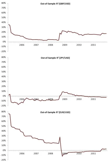
In this section, I test whether predicting forex returns based on the global and the country-specific VRPs outperforms predicting forex returns based on a random walk with drift out-of-sample. I evaluate the performance of the global and country-specific VRPs’ forecasts using an OOS R-square similar to the one proposed by Goyal and Welch (2008). I use a 5-year training sample period from January 2000 to December 2004. The results are reported in Table 11 and displayed in Figure 2. Figure 2 shows that from January 2005 until before the 2008 crisis, the OOS R-squares are positive for GBP and EUR, with a negative slope, which means during this period the historical means smoothly outperform the global and the country-specific VRPs. However, the global and the country-specific VRPs smoothly outperform historical means (positive slope) for JPY in this period.
In the 2008 crisis, the global and country-specific VRPs substantially beat the histor-ical means, and consequently the OOS R-squares are highly positive for all three pairs (they jump up to 8-27%). However, we should note that the high 2008 OOS-R-squares found in this paper are not just due to the low prediction errors of the global and the country-specific VRPs, but they are mainly due to the poor predictive power of the random walk model during the recent crisis.
After the 2008 crisis, the OOS R-squares stay constantly positive for the pound, which means that the global and the country-specific VRPs and historical means have the same performance in predicting GBP/USD forex returns. The OOS R-squares approach zero for Japan and Europe, with negative and positive slopes respectively. In other words, historical means under-perform the global and the country-specific VRPs in Japan and outperform in Europe.
The results of Table 11 show that the final OOS R-square is large and positive for GBP/USD (17%), is small and positive for EUR/USD (2%), and is small and negative for JPY/USD (-2%). More importantly, the final OOS R-square is statistically significant for GBP/USD at the 1% level and for EUR/USD at the 5% level under the McCracken (2007) statistic. The final OOS R-square is not statistically significant. This means equity VRPs significantly outperform the historical mean for GBP/USD and EUR/USD, and they do not significantly under-perform historical means for JPY/USD out-of-sample.26
Moreover, we should note that these OOS performances are based on all three-factor predictions (one global VRP and two country-specific VRPs) together, and that using all
26The global and the country-specific VRPs outperform predicting the exchange rate changes (rather
three factors introduces a lot of noise in the predictions.27
7 Conclusion
This paper provides a way to use forward-looking information available in stock market volatility indices to predict forex returns. By combining the long-run risk with stochastic volatility model of Bollerslev et al. (2009) and the general currency-pricing model of Bekaert (1996) and Backuset al. (2001), I show that expected forex returns are a function of both consumption growth volatilities (as in Bansal and Shaliastovich (2007 and 2013) and Colacito and Croce (2011)) and equity variance risk premiums (VRPs).
Local equity VRPs can be estimated as the difference between the squared volatility indices and the realized variance of the respective equity indices, and therefore they measure aggregate volatility uncertainties. The global VRP is constructed as the average of local equity VRPs in four major countries (the US, UK, Japan and Europe), and thus it captures investors’ common expectations of aggregate volatility uncertainty.
I find that the equity VRPs predict monthly forex returns for the pound, the euro and the yen against the U.S. dollar at the one-month horizon. When I exclude the 2008 crisis months from the sample, the adjusted R-square of predictions for the GBP/USD forex returns decreases, and the significance and explanatory power of the global VRP for the JPY/USD forex returns decrease as well. However, both the adjusted R-square and the significance of the global VRP for the EUR/USD forex returns increase. The significance and explanatory power of the global VRP is mostly unchanged when using Seemingly Unrelated Regressions (SUR), and when including in the regression country-specific and global consumption volatilities. Moreover, even when the local VRPs are unavailable, as is the case for the other 18 currencies in my sample, the global VRP and the US-specific VRP are strong predictors of forex returns for the majority of these currencies with respect to the U.S. dollar. The in-sample predictive power of global and country-specific VRPs extend out-of-sample, where they outperform the standard random walk benchmark. In addition, in a ”horse race” with two strong predictors of currency carry returns—the commodity and the currency volatility factors of Bakshi and Panayotov (2013)—the global VRP has significantly more predictive power for carry returns as well as individual forex returns.
In complete markets with recursive preferences and under lognormality, the models that are used to derive the drivers of equity returns can also be used to determine the factors driving forex returns. More specifically, the cross-country equity premium
differ-27I find that the global VRP has predictive power of in-sample for JPY/USD before the 2008 crisis
entials are driven by the same global and country-specific VRPs and consumption growth volatility factors as the forex returns. This commonality in driving factors provides an explanation for the high degree of contemporaneous comovements between cross-country equity premium differentials and forex returns documented in the data. Moreover, I find that the global VRP is a strong predictor of equity premium differentials, both in the theory and in the data.
References
[1] Andrews, D. W. K. Heteroskedasticity and autocorrelation consistent covariance
matrix estimation. Econometrica 59, 3 (1991), 817–58.
[2] Backus, D., Foresi, S., and Telmer, C. Affine term structure models and the
forward premium anomaly. The Journal of Finance 56, 1 (2001), 279–304.
[3] Backus, D. K., Gavazzoni, F., Telmer, C., and Zin, S. E. Monetary Policy
and the Uncovered Interest Parity Puzzle. NBER Working Papers 16218, National Bureau of Economic Research, Inc, (2010).
[4] Backus, D. K. and Smith, G. W. Consumption and real exchange rates in
dynamic economies with non-traded goods. Journal of International Economics, 35 (1993), 297–316.
[5] Bakshi, G. and Panayotov, G. Predictability of Currency Carry Trades and
Asset Pricing Implications. Journal of Financial Economics 110, 1 (2013), 139–163.
[6] Bansal, R., Khatchatrian, V., and Yaron, A. Interpretable asset markets?
European Economic Review 49, 3 (2005), 531 – 560.
[7] Bansal, R., and Shaliastovich, I. Risk and return in bond, currency, and
equity markets. working paper, Duke University, (2007).
[8] Bansal, R., and Shaliastovich, I. A Long-Run Risks Explanation of
Pre-dictability Puzzles in Bond and Currency Markets. Review of Financial Studies 26
1 (2013), 1–33.
[9] Beeler, J., and Campbell, J. Y. The long-run risks model and aggregate asset
prices: An empirical assessment. NBER Working Papers 14788, National Bureau of Economic Research, Inc, (2009).
[10] Bekaert, G. The time variation of risk and return in foreign exchange markets: A
general equilibrium perspective. Review of Financial Studies 9, 2 (1996), 427–70.
[11] Bekaert, G., and Hodrick, H. Characterizing Predictable Components in
Ex-cess Returns on Equity and Foreign Exchange Markets. The Journal of Finance 47, 2 (1992), 467–509.
[12] Bekaert, G., and Hoerova, M. The VIX, the variance premium and stock
[13] Benigno, G. Real exchange rate persistence and monetary policy rules. Journal of Monetary Economics 51, (2004), 473–502.
[14] Bollerslev, T., Marrone, J., Xu, L., and Zhou, H. Stock return
predictabil-ity and variance risk premia: Statistical inference and international evidence.Journal of Financial and Quantitative Analysis, Forthcoming (2014).
[15] Bollerslev, T., Tauchen, G., and Zhou, H. Expected stock returns and
variance risk premia. Review of Financial Studies 22, 11 (2009), 4463–4492.
[16] Brunnermeier, M. K., Nagel, S., and Pedersen, L. H. Carry trades and
currency crashes. Tech. rep., National Bureau of Economic Research, (2008).
[17] Burnside, A. C. and Graveline, J. J. On the Asset Market View of Exchange
Rates. NBER Working Papers 18646, National Bureau of Economic Research, Inc, (2012).
[18] Campbell, J., and Shiller, R. The dividend-price ratio and expectations of
future dividends and discount factors. Review of financial studies 1, 3 (1988), 195– 228.
[19] Cappiello, L., and De Santis, R. A. Explaining exchange rate dynamics: The
uncovered equity return parity condition. SSRN eLibrary (2005).
[20] Carr, P., and Wu, L. Variance risk premiums. Review of Financial Studies 22,
3 (2009), 1311–1341.
[21] Chinn, M., and Meese, R. Banking on currency forecasts: how predictable is
change in money? Journal of International Economics 38, (1995), pp. 161–178.
[22] Cochrane, J. H. Discount rates. Journal of Finance 66, (2011), pp. 1047–1108.
[23] Colacito, R., and Croce, M. M. Risks for the long run and the real exchange
rate. Journal of Political Economy 119, 1 (2011), 153–181.
[24] Cooper, I., and Priestley, R. Time-varying risk premiums and the output gap.
Review of Financial Studies 22, 7 (2009), 2801–2833.
[25] Constantinides, G. M., and Ghosh, A. Asset pricing tests with long-run risks
in consumption growth. Review of Asset Pricing Studies 1, 1 (2011), 96–136.
[26] Del Negro, M. Aggregate risk sharing across us states and across european
[27] Del Negro, M. Asymmetric shocks among u.s. states. Journal of International Economics 56, 2 (2002), 273–297.
[28] Della Corte, P., Ramadorai, T. and Sarno, L. Variance risk premiums and
Exchange Rate Predictability. SSRN eLibrary, (2014).
[29] Drechsler, I., and Yaron, A. What’s vol got to do with it. Review of Financial
Studies 24, 1 (2011), 1–45.
[30] Eichenbaum, M. S., and Evans, C. L. Some empirical evidence on the effects
of monetary policy shocks on exchange rates. Quarterly Journal of Economics 110, (1995), 975–1009.
[31] Engel, C., and West, K. D. Taylor rules and the deutschmark-dollar real
exchange rate. Journal of Money, Credit and Banking 38, (2006), 1175–1194.
[32] Epstein, L. G., and Zin, S. E. Substitution, Risk Aversion, and the Temporal
Behavior of Consumption and Asset Returns: A Theoretical Framework. Economet-rica 57, 4 (1989), 937-969.
[33] Epstein, L. G., and Zin, S. E. Substitution, Risk Aversion, and the Temporal
Behavior of Consumption and Asset Returns: An Empirical Analysis. Journal of Political Economy 99, 2 (1991), 263–286.
[34] Ferreira, M. A., and Santa-Clara, P.Forecasting stock market returns: The
sum of the parts is more than the whole. Journal of Financial Economics 100, 3 (2011), 514–537.
[35] Goyal, A., and Welch, I. A comprehensive look at the empirical performance
of equity premium prediction. Review of Financial Studies 21, 4 (2008), 1455–1508.
[36] Gourio, F., Siemer, M., and Verdelhan, A. International risk cycles. Journal
of International Economics 89, 2 (2013), 471–484.
[37] Hasseltoft, H. Stocks, bonds, and long-run consumption risks. Journal of
Fi-nancial & Quantitative Analysis 47, 2 (2012), 309 – 332.
[38] Hau, H., and Rey, H. Exchange rates, equity prices, and capital flows. Review of
Financial Studies 19, 1 (2006), 273–317.
[39] Hess, G. D., and Shin, K. Intranational business cycles in the united states.
[40] Hess, G. D., and Shin, K. Understanding the backus-smith puzzle: It’s the (nominal) exchange rate, stupid. Journal of International Money and Finance 29, 1 (2010), 169–180.
[41] Lauterbach, B. Consumption volatility, production volatility, spot-rate volatility, and the returns on treasury bills and bonds. Journal of Financial Economics 24, 1 (1989), 155–179.
[42] Londono, J.-M., and Zhou, H.Variance risk premiums and the forward premium
puzzle. SSRN eLibrary, (2012).
[43] Lustig, H., and Nieuwerburgh, S. V. How much does household collateral
constrain regional risk sharing? Review of Economic Dynamics 13, 2 (2010), 265– 294.
[44] Lustig, H., Roussanov, N., and Verdelhan, A. Countercyclical currency risk
premia. Journal of Financial Economics 111, 3 (2014), 527–553.
[45] Lustig, H., Roussanov, N., and Verdelhan, A. Common risk factors in
currency markets. Review of Financial Studies 24, 11 (2011), 3731–3777.
[46] Lustig, H., and Verdelhan, A. The cross section of foreign currency risk premia
and consumption growth risk. American Economic Review 97, 1 (2007), 89–117.
[47] McCracken, M. Asymptotics for out of sample tests of Granger causality. Journal
of Econometrics 140, (2007), 719–752.
[48] Meese, R. A., and Rogoff, K. Empirical exchange rate models of the seventies:
Do they fit out of sample? Journal of International Economics 14, 1-2 (1983), 3–24.
[49] Menkhoff, L., Sarno, L., Schmeling, M., and Schrimpf, A. Carry trades
and global foreign exchange volatility. Journal of Finance 67, 2 (2012), 681–718.
[50] Mueller, P., Vedolin, A., and Zhou, H. Short-run bond risk premia. SSRN
eLibrary (2011).
[51] Newey, W. K., and West, K. D. A simple, positive semi-definite,
heteroskedas-ticity and autocorrelation consistent covariance matrix. Econometrica 55, 3 (1987), 703–08.
[52] Ostergaard, C., Serensen, B. E., and Yosha, O.Consumption and aggregate
[53] Rogoff, K. Exchange rates in the modern floating era: what do we really know?
Review of World Economics 145, 1 (2009), 1–12.
[54] Rogoff, K. S., and Stavrakeva, V. The continuing puzzle of short horizon
ex-change rate forecasting. NBER Working Papers 14071, National Bureau of Economic Research, Inc, (2008).
[55] Santa-Clara, P., and Yan, S. Crashes, volatility, and the equity premium:
Lessons from s&p 500 options. The Review of Economics and Statistics 92, 2 (2010), 435–451.
[56] Stulz, R. A model of international asset pricing. Journal of Financial Economics
9, 4 (1981a), 383–406.
[57] Stulz, R. On the effects of barriers to international investment. Journal of Finance 36, 4 (1981b), 923–934.
[58] Verdelhan, A. A habit-based explanation of the exchange rate risk premium.
Journal of Finance 65, 1 (2010), 123–146.
[59] Verdelhan, A.The share of systematic variation in bilateral exchange rates.SSRN
eLibrary (2012).
[60] Wilcox, D. W. Social security benefits, consumption expenditure, and the life
cycle hypothesis. Journal of Political Economy 97, 2 (1989), 288–304.
[61] Zellner, A. An efficient method of estimating seemingly unrelated regressions and
tests for aggregation bias. Journal of the American Statistical Association 57, 298 (1962), pp. 348–368.
[62] Zhou, H. Variance risk premia, asset predictability puzzles, and macroeconomic
Appendix A
The details of derivation for Equation 16 are as follows:
var[mt+1] =var[θlog(δ)−
θ
ψgt+1+ (θ−1)rt+1]
= (θ
ψ)
2
var(gt+1) + (θ−1)2var(rt+1)−2(
θ
ψ)(θ−1)cov(gt+1, rt+1)
= (θ
ψ)
2
σg,t2 + (θ−1)2(σg,t2 +κ12(Aσ2+Aq2ϕq2)qt)−2(
θ
ψ)(θ−1)σ
2
g,t
= ((θ
ψ)
2
+ (θ−1)2−2(θ
ψ)(θ−1))[σ
2
g,t] + (θ−1)
2
κ12(Aσ2 +Aq2ϕq2)[qt] therefore,
var[mt+1] =γ2[σ2g,t] + (θ−1)
2


![MMA Capital Management, LLC [MMAC] Q Earnings Conference Call Friday, November 14, 2014, 8:30 a.m. ET](data:image/gif;base64,R0lGODlhAQABAIAAAP///wAAACH5BAEAAAAALAAAAAABAAEAAAICRAEAOw==)