Low Versus High Leverage (LVH)

Munich Personal RePEc Archive

Low Versus High Leverage (LVH)

Bebel, Arkadiusz

Warsaw School of Economics

8 November 2014

Online at

https://mpra.ub.uni-muenchen.de/62889/

Low Versus High Leverage (LVH)

Arkadiusz Bebel

This draft: 8.11.2014

Abstract

Disputes whether financial structure can create value or not were started more than 50 years

ago with Modigliani Miller theorem. In this paper I would like to present my own view on level of

debt in value creation process. What I am going to prove is that due to expansion option

companies with low level of debt are outperforming highly leveraged companies in the long run.

I have created a new factor LVH (low versus high leverage) to quantitatively prove that being long

in companies with below median net debt/EBITDA and being short in companies with above net

debt/EBITDA can bring abnormal returns (with Sharpe ratio even higher than 0.9 and statistically

significant alfa of around 7.7% yearly). As shown in chapter IV.II. such strategy might be

supplemented by Momentum, Betting against Beta or High minus Low Devil strategies.

Page | 2

Contents

I. Introduction ... 3

II. Level of debt as a single factor ... 5

III. Methodology of research ... 10

IV. Results of research... 12

IV. I. Analysed portfolios and markets ... 13

IV. I. I. US & Canada... 13

IV. I. II US & Canada – monthly data ... 20

IV. I. III. Europe ... 23

IV. I. IV. Japan ... 27

IV. I. V. Asia & Australia ... 30

IV. II. Risk adjusted returns ... 33

V. Findings ... 38

Bibliography ... 39

List of Tables ... 42

Page | 3

I. Introduction

Factor investing is developing since at least 50 years and currently it seems to be the fastest developing area of investment theory. From historical point of view first factor investing model was CAPM (Treynor

– 1961,1962; Sharpe – 1964; Lintner – 1965; Mossin – 1966), which main factors are systematic and idiosyncratic risks. Then development of theories started through APT theory2 _{and Fama and French three}

factor model. Currently researchers are looking for new factors which might explain movements of share prices e.g. Betting against Beta (BAB factor) or Quality Minus Junk (QMJ). Some factors for some sectors are unrelated strictly to financial issues e.g. number of users proposed by professor A. Damodaran3_.

Factor investing is gaining on popularity not only among academics but also in practice. Several investment strategies which base on different factors were created. According to Foundations of Factor Investing4 _{the most popular strategies base on such factors:}

 Value (buying companies with low market cap in comparison to fundamental value, so low P/E, P/BV etc.)

 Size (gaining excess return on being long in small companies and short in long companies, known as a SMB – small minus big – in Fama-French three-factor model)

 Momentum (investing in companies with stronger past performance, according to saying “trend

is your friend”

 Volatility (invest in companies with low volatility, beta)

 Dividends yield (capturing excess return of companies with high dividend yields)  Quality (invest in companies with strong balance sheet, high ROE, low debt etc.)

As we can see factors presented above more or less depends on share prices (market caps), which might be a fundamental drawback of such strategies. This is because in most cases current share price do not influence operational activities in a company and its growth. I do not neglect the theory, that it is possible to obtain abnormal returns basing on trading factors. I want to propose another theory, that fundamental factors are at least equally probable to bring investment strategy which presents long term abnormal profits as trading factors. This is because fundamental factors are connected with real value. Such observation was a starting point for my research of a new “only fundamental” factor.

Factor investing strategy “quality” is the closest to the idea of only fundamental factor(s), but there is no single data which strictly measures quality, rather there are some combinations of fundamental factors to assess quality of company. According to MSCI Quality Indices Methodology: Quality growth companies are characterized in the literature as companies with durable business models and sustainable competitive

2 _{ROSS, Stephen A. The arbitrage theory of capital asset pricing. Journal of economic theory, 1976, 13.3: 341-360.} 3 _{http://aswathdamodaran.blogspot.com/2014/02/facebook-buys-whatsapp-for-19-billion.html}

Page | 4

advantages. Quality growth companies tend to have high ROE, stable earnings that are uncorrelated with the broad business cycle, and strong balance sheets with low financial leverage.5

There are three factors included in MSCI Quality Index – ROE, debt to equity ratio and earnings variability. I am not fully convinced whether these factors fully represent quality of company. In calculation of debt to equity ratio there is a book value of equity taken into account, whereas from practical point of view market cap is better representing current value of equity. However taking market cap also might be confusing, because growing share price will make debt to market cap ratio to decline, which is at least partially coherent with momentum strategy (investing in a company after a good period) and might create a bias. Last factor – earnings variability is also disputable, because companies with completely flat results

shouldn’t be preferred in the long run to companies with growing, but a little bit volatile results.

Another world well-known quality index is Global Quality Income Index presented by Societe Generale Cross Asset Research6_{. There should be at least seven out of nine criteria presented below fulfilled for a}

company to be qualified to the index. Criteria are divided into three categories:

 Profitability factors (positive ROA, positive CFO, growing ROA, negative accruals)

 Leverage, liquidity, source of funds (declining leverage, growing liquidity, no share issues in analysed period)

 Operating efficiency (growing margins, growing turnover)

As we can see also in this methodology there are several ratios which measure quality and it seems justified to analyse them separately as a possible factors to investment strategies. Such analysis for gross profitability was done by Novy-Marx (2013). The main finding was high negative correlation between strategies based on gross profitability and price signals. The other finding was the fact that strategies which base on gross profitability has as much power in predicting stock returns as presented before traditional value metrics.7

Another separate factor to measure quality of the company is strength of balance sheet. Several ratios can be calculated but to my mind one of the most important is level of debt, which was partially analysed in this paper.

5 _{MSCI Quality Index Methodology published in May 2013, can be found here:}

http://www.msci.com/eqb/methodology/meth_docs/MSCI_Quality_Indices_Methodology.pdf 6 _{Global Quality Income Index The Methodology presented by Societe Generale, can be found here:} http://www.solactive.com/downloads/DE000SLA3SG6_leitfaden.pdf

Page | 5

II. Level of debt as a single factor

The current macroeconomic situation with very low interest rates makes external financing cheap, but external sources of financing are obtainable only for not so highly leveraged companies. That is why low leveraged companies can gain fundamental advantage over highly leveraged ones because of “on debt” expansion option. This finding was a basic principle to check, whether there is observable premium to be gained by investing in low leveraged companies. Further I will call the strategy of being long in low indebted companies and being short in high indebted companies as LVH strategy (LVH = Low Versus High, described in details in part III. Methodology).

Taking level of debt as a factor in investment strategies has advantages that it has strong background in theoretical disputes and can be empirically checked for many markets/sectors/periods of time. In this chapter I will present fundamental issues which are in my opinion underestimated by investors and then in the next chapter I will show results of empirical research.

In presented in chapter one quality investment strategies level of debt was (sometimes) a part of a strategy. I would like to emphasize one significant difference between my research and what have been done before. In previous researches there were analysed ratios (or some combinations of ratios) like total debt/book value of equity; debt to assets etc. In my research I will analyse ratio of net debt to EBITDA as a single factor. This is because such ratio is commonly known covenant for credit financing and better

reflects company’s credibility.

A lot have been said whether capital structure can create a value or not. According to Modigliani-Miller model8 _{capital structure does not affect value (I assume that there are no taxes), which more or less is}

true (it is not a matter of this paper to discuss this issue in details). What I think is that capital structure does not affect value in short term, but companies with low net debt to EBITDA are able to gain additional financing to accelerate development in favourable times (expansion option). Obviously such possibility has a higher value for not so highly leveraged companies. I think that classical MM theorem (without taxes, in case of taxes tax shield should be added) should be converted as presented below:

𝑉𝑎𝑙𝑢𝑒 𝑜𝑓 𝑙𝑒𝑣𝑒𝑟𝑒𝑑 𝑐𝑜𝑚𝑝𝑎𝑛𝑦 = 𝑉𝑎𝑙𝑢𝑒 𝑜𝑓 𝑢𝑛𝑙𝑒𝑣𝑒𝑟𝑒𝑑 𝑐𝑜𝑚𝑝𝑎𝑛𝑦 + 𝑣𝑎𝑙𝑢𝑒 𝑜𝑓 𝑒𝑥𝑝𝑎𝑛𝑠𝑖𝑜𝑛 𝑜𝑝𝑡𝑖𝑜𝑛

What I am going to argue is that investors underestimate value of expansion option (which should be understand as an option to gain additional external financing to accelerate growth) and investing in

8_{MODIGLIANI, Franco; MILLER, Merton H. The cost of capital, corporation finance and the theory of}

Page | 6 indebted companies (by low indebted companies I understand also companies with net cash position) can bring abnormal return.

To proof this thesis from theoretical point of view life cycle of company should be analysed. At the beginning there is an idea and some sources of internal financing (initial capital). This is because credibility of company is low and it is almost impossible to gain significant external debt financing. As company is growing and there are good opportunities to accelerate development company may use external financing

(I assume that on “higher” stage of life cycle access to external financing is easier). On the other side if there are not so promising opportunities then company should not issue debt and we are in previous state of unleveraged company. If entity decides to increase its financial leverage and project goes in line with assumptions then company is growing faster than it would in case of self-financing. Then if company is generating excess cash it has also a possibility to invest or to repay debts. I think that such situation might be a good example to measure a quality of management board. If board expects macro conditions to deteriorate it is reasonable to decrease financial leverage and accumulate some cash for crisis (for e.g. attractive takeovers). As we can see from above example a low-indebted company can accelerate its development in good conditions and decrease leverage in expectations of macro deterioration. Such decrease of leverage might be a good base for a next growth period. Summing up, from life cycle theory low leveraged companies should outperform highly leveraged ones.

From behavioral point of view also low leveraged companies should be preferred (with some short time exceptions). When stock market is at the peak and crisis begins investors should get rid of highly leveraged companies because of higher risk of bankruptcy. Then I suppose that for a really short period of time highly leveraged companies might outperform low-indebted ones because of lower basis and stronger sell-off during declines. Although this thesis is rational there is no evidence in conducted research that low-indebted companies underperform highly leveraged ones even in short term (as presented in chapter IV. II. market premium factor – so market situation – is not statistically significant in modelling returns of LVH strategy). From behavioral point of view this thesis about potential outperformance of low leveraged companies is also disputable. Just after a crisis prospects for high quality companies should be better than for low quality companies (stronger balance sheet, better market position). Moreover low leveraged companies have more possibilities to gain capital for acceleration of development. Also it should be emphasized that investors are biased and after a crisis it is easier to invest in safer assets/companies. All these statements are in favour of theory that low leveraged companies should outperform leveraged ones at the beginning of economic recovery. As markets are growing I claim that low leveraged companies continue to increase valuation gap till the point the valuation of low leveraged companies is getting too high and investors are looking for alternatives. This is mainly in the last part of bull market, where investors feel less risk aversion and invest in lower quality, higher leveraged and more risky companies. For this short period of time highly leveraged companies might outperform low leveraged companies. Summing up, from stock market cycle analysis I would expect low leveraged companies to outperform high leveraged ones for a whole cycle with exception of last part of bull market. What can be seen in chapter IV. II. for about 70% of time strategy brought satisfactory results, which is in line with expectations.

Page | 7 like dividends or volatility works, but maybe LVH factor is statistically important in explaining them). For example as it comes to value strategy I tried to prove that lower-indebted companies can obtain higher growth rate, so even if multiples like P/E or EV/EBITDA are similar now for different companies Then if we calculate current market cap or enterprise value to future earnings or EBITDA lower-indebted companies should be cheaper and with elapse of time share prices should grow faster. Secondly, as companies with low net debt are less risky so volatility of shares should be lower.That is why such companies should be also preferred in low volatility factor investment strategy. Thirdly an ability to pay high dividends for low-indebted companies is higher than for highly leveraged companies, which also is in line with stated thesis about outperformance of low-leveraged companies. Finally, it is more probable for low indebted companies to be high quality companies, with strong balance sheet. Also according to pecking order theory

there is a negative correlation between level of debt and profitability of company, which proofs on average higher quality of low-indebted companies.9

If we look at theory and explanations of excess returns for popular factor investment strategies there are several explanations presented. According to Exhibit 5: Theories behind the Excess Returns to Systematic Factors presented in Foundations of Factor Investing by MSCI, December 2013:

Systematic

Factor Systematic Risk-based theory Systematic Errors-based Theories

Value - Higher systematic (business cycle) risk

- Errors in expectations - Loss aversion

- Investment-flows-based theory

Low Size (Small Cap)

- Higher systematic (business cycle) risk

- Proxy for other types of systematic risk - Errors in expectations

Momentum - Higher systematic (business cycle) risk

- Higher systematic tail risk

- Underreaction and overreaction - Investment-flows-based theory

Low Volatility N/A

- Lottery effect

- Overconfidence effect - Leverage aversion

Dividend Yield - Higher systematic (business cycle) risk - Errors in expectations

Quality N/A - Errors in expectations

Page | 8

Table 1 Explanations of excess returns for popular factor investment strategies, based on The Exhibit 5: Theories behind the Excess Returns to Systematic Factors presented in Foundations of Factor Investing by MSCI, December 2013

While analysing this table “so what?” question should be asked. For example while analysing value as an systematic factor we can see higher systematic (business cycle) risk as an explanation. So what? So if company is more risky, then gaining debt should be more difficult and company should finance more activities with internal sources of funding. In such way some of systematic factors can be explained as a derivative of level of debt.

As it comes to scientific papers related to this field of research there is an interesting and seemingly uncorrelated paper Betting against Beta by Andrea Frazzini and Lasse Heje Pedersen10_{. The main thesis of} this paper is that being long in leveraged low-beta assets and short high beta assets from statistical point of view can bring abnormal returns. There are several explanations presented and proved, but I would like to shed a new light on this research. The main two factors which affects beta are: business factors

(industry, stage of company etc.) and financial factors (which leverage “typical” unleveraged beta for an industry). Analysing undecomposed betas do not bring answer whether being long in leveraged low-beta assets and short high beta assets is due to an industry or due to financial leverage. In my paper I claim that being long in unleveraged companies and short in leveraged companies is bringing abnormal profit in the long run, which is only partially in line with thesis stated in that paper. Let’s assume that there is a simple economy with only two sectors: IT (high sector beta) and utilities (low sector beta), and companies among sectors substantially vary as it comes to leverage. I assume in model that the smallest beta of company from IT sector is higher than the highest beta of utilities to make series of data separable.

And now the question which should be answered is: Is it better to be short IT and long utilities (with leverage) or is it better to be long low-indebted IT & Utilities and short highly-indebted IT & Utilities. According to the paper Betting against beta the first is true. If that’s true, then there should exist low beta sectors which if leveraged almost permanently outperform other sectors.

In my low debt factor investing approach second answer is better way of investing. In my theory low-indebted companies are able to develop faster so being long low-low-indebted IT & Utilities and short high-indebted IT & Utilities brings better exposition on potential future market leaders (faster growing companies).

The other issue which should be emphasized is that being leveraged in unleveraged company is quite different than being unleveraged in leveraged company, although from mathematical point of view beta might be the same. This is because leveraging investor’s position do not create inflow of money to the company, while changing financial leverage in company might create some changes in cash flows. As I am analysing performance of shares I am interested in process of changing leverage in companies and its impact on performance. The possibility of changing leverage by investor in fact does not matter, because if unleveraged strategy brings abnormal profit then any investment leverage will bring abnormal profit as well (if cost of financing is lower than return of the strategy).

Page | 10

III. Methodology of research

The data for this research were collected from the CRSP®/Compustat Merged Database. Then empirical analysis of performance of companies in dependence on level of net debt to EBITDA was conducted. Analysis was done in yearly interval for most developed markets and moreover in monthly interval for US & Canada. Net debt was taken at the end of fiscal year and market caps were taken at 1st _{April. Such}

construction allows implementation of strategy in practice (only a small percent of companies publish yearly financial statement after 1st _{April so there is a practical availability of data for the 1}st _April –

companies present financial statements with delay, normally no more than 3 months). Corporate events like dividends/buybacks etc. were taken into account while calculating performance. All yearly returns are presented in local currencies, as currency changes are not the aim of this research. The data were filtered and companies with share price lower than 1 USD for US & Canadian market and below 0,5 unit of local currency for other markets were omitted. To make ratio of net debt/EBITDA applicable also companies with reported negative EBITDA were omitted. It should be emphasized, that ratio of net debt/EBITDA might be both very high or very low in case when EBITDA is positive (close to zero) and company has a net cash or net debt position. That is why I was analysing medians not averages. In case when several series of shares were quoted author took into consideration only one series (otherwise one company could be double-counted).

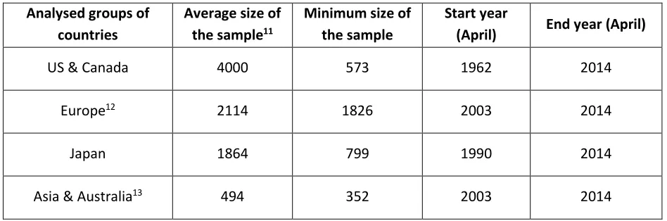
As analysed samples should be big enough to bring statistically important results I divided developed markets as follows:

Analysed groups of countries

Average size of the sample11

Minimum size of the sample

Start year

(April) End year (April)

US & Canada 4000 573 1962 2014

Europe12 _{2114 1826 2003 2014}

Japan 1864 799 1990 2014

Asia & Australia13 _{494 352 2003 2014}

Table 2 Analesed groups of countries and main parameters

11 _{This is a number of companies which were analysed for portfolios so: they were quoted on year x and x+1,} financial data (both net debt and EBITDA) were available in CRSP®/Compustat Merged Database, EBITDA in year x was greater than zero, share price in year x was bigger than 1 USD or 0,5 unit of local currency. Surely whole universe of analysed companies before filters were implemented was much bigger (analysing companies with negative EBITDA is senseless as it comes to net debt/EBITDA ratio so filters are needed)

12 _{Includes: Austria, Belgium, Switzerland, Germany, Denmark, Spain, Finland, France, Great Britain, Italy,} Netherlands, Norway, Sweden

Page | 11 All analysed portfolios were equal weighted and dollar neutral. Taking equal weighted portfolios is justified by the fact, that I want to exclude size factor in my analysis. Second condition which are dollar neutral portfolios is justified by the fact that I want to compare performance of highly indebted companies versus low indebted ones. I do not assume that being long only low indebted strategies will always bring positive return, but that such strategy will outperform being short in high indebted companies. Moreover dollar neutral strategies makes comparison to other strategies easier (e.g. no problem with choosing appropriate benchmark). As this is dollar neutral strategy in calculation of Sharpe ratio there is no need to subtract risk-free rate (I am calculating factor premium).

For every sample I analysed four different equal weighted portfolios

 Being long in below median companies and being short in above median company - further as a

50/50portfolio

 Being long in below 25th _{percentile companies and being short in above 75}th _{percentile companies}

- further as a 25/75portfolio

 Being long in below 10th _{percentile companies and being short in above 90}th _{percentile companies} – further as a 10/90portfolio

 Being long from 5th _{to 50}th _{percentile companies and being short in above 50}th _{to 95}th _percentile

companies (to exclude potential impact of highly marginal data) - further as a 5-50/50-95portfolio

As it comes to potential biases of this research some issues should be emphasized. First is existence of survivorship bias, which is in fact difficult to be avoided in any research based on historical data. I took into consideration only companies which were quoted both on year x and x+1, which seems to be a common practice. Nevertheless it should be remembered that for some years (e.g. 2001), when many companies went bankrupt results from analysed strategy might be biased (on the other hand there are still big samples analysed). Second risk associated with research are potential drawbacks of data sources

– there is a risk that some market data are not or incorrectly included in the CRSP®/Compustat Merged Database (again taking big sample makes this risk small). Transaction costs and taxes were not included in analysis.

Page | 12

IV. Results of research

Results of research are in line with expectations – companies with lower debt on average outperformed companies with higher debt. In tables below there are presented results for different portfolios as it comes to average return in analysed period, standard deviation of returns and Sharpe ratio.

Average return in

analysed period US & Canada Europe Japan Asia & Australia

50/50 portfolio 5,01% 9,52% 3,41% 11,36%

25/75 portfolio 7,48% 15,56% 6,10% 13,79%

10/90 portfolio 9,27% 20,16% 8,85% 13,96%

5-50/50-95 portfolio 4,62% 7,99% 2,68% 10,66%

Table 3 Average return in analysed period for different portfolios and markets

As we can see from above table average returns for dollar neutral portfolios vary substantially among regions and portfolios, but were on average always positive in a long term. Moreover if we compare first three portfolios (50/50; 25/75; 10/90) there is observable monotonicity. Playing unleveraged companies vs strongly leveraged companies brings better results as more extreme intervals are taken. This is consistent with presented in part II theory – low indebted companies are undervalued vs high indebted companies.

St. deviation of returns US & Canada Europe Japan Asia & Australia

50/50 portfolio 8,36% 8,31% 7,26% 10,17%

25/75 portfolio 13,40% 12,24% 10,15% 9,33%

10/90 portfolio 17,53% 20,50% 9,84% 14,16%

5-50/50-95 portfolio 7,52% 6,16% 7,40% 11,10%

Table 4 Standard deviation of returns in analysed period for different portfolios and markets

Page | 13

Sharpe ratio US & Canada Europe Japan Asia & Australia

50/50 portfolio 0,60 1,15 0,47 1,12

25/75 portfolio 0,56 1,27 0,60 1,48

10/90 portfolio 0,53 0,98 0,90 0,99

5-50/50-95 portfolio 0,61 1,30 0,36 0,96

Table 5 Sharpe ratio in analysed period for different portfolios and markets

As it comes to Sharpe ratios (which for dollar neutral portfolios are calculated as an average return divided by standard deviation of returns) it is quite different for portfolios & markets. To my mind Sharpe ratio presented above is quite rewarding, which affirms the conviction about long term abnormal profits to be gained from investing in not so highly leveraged companies and being short in highly leveraged ones.

Comparing to other quantitative strategies Sharpe ratio presented above also brings satisfactory results. In paper Betting Against Beta authors present Sharpe ratio of their strategy to be 0.78 (for US Market, years 1926-2012). This is twice that of the value effect (so around 0.40), and 40% higher than momentum (so around 0.56).14 _{As we can see for US & Canada results as it comes to Sharpe ratio are better than for}

value and momentum strategies and a little bit worse than for BAB (Betting Against Beta) factor. For other markets like Asia & Australia results seems even more promising however time range of analysis due to accessibility of data is shorter. Moreover it should be remembered that my analysed strategy is dollar-neutral, BAB strategy is market-neutral and momentum and value strategies are very often long strategies (or dollar-neutral), but almost never market-neutral.

In the following chapters results for particular markets and portfolios are discussed in details.

IV. I. Analysed portfolios and markets

IV. I. I. US & Canada

The first analysed market was US & Canadian market, which is the biggest market and availability of historical data is the broadest. The whole backtesting universe contains more over 20 000 companies, which after filtering for restrictions described in chapter III brings on average 4 000 companies per year. The analysed period is from April 1962 till April 2014 (as it comes to further notation there is only first year given, for example period from April 1970 to April 1971 will be named as 1970).

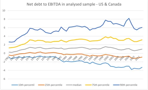
Page | 14 Whole idea of analysis is to assess impact of net debt/EBITDA on return on investments. As we can see from chart presented below level of net debt/EBITDA is quite stable over time especially as it comes to median value. As sample increases over time (from min 573 in 1962 to more than 6300 in 1997) it is natural that marginal percentiles for net debt/EBITDA will widen over time. Moreover it should be emphasized that as economic situation decreases and financial results are weaker then net debt/EBITDA should naturally increase. However on the other site companies which EBITDA falls below 0 are excluded from research.

Figure 1 Net debt/EBITDA in analysed sample – US & Canada

As it comes to popular banking covenants in creditworthiness assessment process one of the most popular is net debt/EBITDA of around 3-4, which is in line with chart presented above, where around 75% of companies have such factor below 4, which might be interpreted as their leverage is under reasonable control.

Average returns for analysed strategies are presented below. Not only strategies bring very good results as it comes to average return, but also number of years in which results of being long in low leveraged companies and being short in high leveraged companies is satisfactory – more than 70% of time.

Portfolio Average return

St. Deviation

of returns Sharpe ratio

% of positive results

50/50 portfolio 5,01% 8,36% 0,60 76,92%

-6 -4 -2 0 2 4 6 8 10

Net debt to EBITDA in analysed sample - US & Canada

Page | 15

25/75 portfolio 7,48% 13,40% 0,56 73,08%

10/90 portfolio 9,27% 17,53% 0,53 73,08%

5-50/50-95 portfolio 4,62% 7,52% 0,61 78,85%

Table 6 Performance of different portfolios in US & Canada

If we look at a chart presented below which shows results over time for different strategies high volatility is observable from 1999 to 2004. Results of strategy for one year around 100% return seems impossible, but when we look deeply insight it is OK.

Figure 2 Decomposed results of analysed portfolios – US & Canada

Years 1999-2004 it was a period of dot-com bubble, where many Internet companies were created. Such companies had normally little debt (as a credibility of technological companies in a seed stage is lower for banks) and some positive EBITDA, so they were classified into analysed sample. Then it should be emphasized that I analyse equal weighted portfolios (to exclude size factor), so as the number dot-com companies increases they are most probably included in low indebted portfolios. Then growth in the last part of cycle should be mentioned “The dot-com bubble burst, numerically, on March 10, 2000, when the technology heavy NASDAQ Composite index peaked at 5,048.62 (intra-day peak 5,408.60), more than

-0.4 -0.2 0 0.2 0.4 0.6 0.8 1 1.2

Results of analysed portfolios - US & Canada

Page | 16

double its value just a year before.”15_{. As index more than doubled and it was dot-com boom we can}

assume that in the last period dot-com companies outperformed classical companies (e.g. mining, utilities etc.), so now difference seems reasonable. Then dot-com companies which were low leveraged dropped more, because of unreasonable valuation before, so portfolio brought negative profit. Moreover in that time so many companies went bankrupt, which make bias in this research. In the following years situation come back slightly to normality. As we can see in 2003 low leveraged companies strongly outperformed highly leveraged ones, which is in line in theory presented in chapter II (risk aversion after crisis makes low indebted companies to gain abnormal profits in recovery period).

Dot-com bubble was somehow special – it was not a crisis which burst by over borrowing and then Minsky moment. Such event in data analysis process for this strategy is beneficial, because it discloses downside risk which might occur in particular years. As presented in table below even dollar-neutral strategy might bring substantial losses even up to 30%. However if we look at strategy in longer period such losses are fully compensated by profits in other years.

1999 2000 2001 2002 2003

50/50 portfolio 42.34% -9.13% 7.32% 0.27% 20.25%

25/75 portfolio 67.30% -24.62% 12.19% -1.83% 34.36%

10/90 portfolio 94.69% -27.44% 14.18% -8.45% 53.26%

5-50/50-95

portfolio 35.47% -5.82% 6.15% 1.63% 15.25%

Table 7 Performance of different portfolios in US & Canada in years 1999-2003

For scientific purposes I also analysed the same strategy excluding period 1.04.1999 – 31.03.2004. Results are presented in separate section later in paper.

For factor investment strategy to be consistent it is also recommended to observe monotonicity in deciles / quantiles. Conducted research shows that higher deciles, so companies with higher net debt/EBITDA on average presents worse results than companies from lower deciles, but strict monotonicity is not observable for US & Canadian market. Obviously if we compare 5th _{with 6}th _{decile, 4}th _{with 7}th _{lower deciles}

are preferable, but e.g. 3rd _{is preferable to 2}nd _{(but the difference is not so high).}

The highest Sharpe ratio is for 3rd _{and 4}th _{decile, which might be justified as these are companies which}

use some debt but not a lot and there is still an expansion option to be priced. On the other hand companies from 1st _{decile might be reluctant to take any debt even in case of extraordinary opportunity,}

so that is why they do not obtain as high abnormal profit as a little bit more indebted companies.

Average return St. Deviation of returns Sharpe ratio

Page | 17

1st _{decile 15,88% 28,33% 0,56}

2nd _{decile 18,87% 26,87% 0,70}

3rd _{decile 17,72% 23,81% 0,74}

4th _{decile 18,56% 24,75% 0,75}

5th _{decile 16,98% 23,74% 0,72}

6th _{decile 15,86% 24,05% 0,66}

7th _{decile 14,89% 25,53% 0,58}

8th _{decile 13,96% 24,63% 0,57}

9th _{decile 11,63% 24,92% 0,47}

10th _{decile 6,59% 24,41% 0,27}

Table 8 Decomposition of returns in deciles – US & Canada

Below there is presented visualisation of above table. The Sharpe ratio curve is quite characteristic and similar for different analysed markets.

Figure 3 Average key parameters for deciles in US & Canada

0.00% 10.00% 20.00% 30.00% 40.00% 50.00% 60.00% 70.00% 80.00%

1st decile 2nd decile 3rd decile 4th decile 5th decile 6th decile 7th decile 8th decile 9th decile 10th decile

Average key parameters for deciles in US & Canada (1962-2014)

Page | 18 Summing up results for US & Canada in years 1962-2014 it seems that strategy of being long in low leveraged companies and being short in high leveraged companies brought a very good results both as it comes to average rate of return and Sharpe ratio.

IV. I. I. I. Without period 1.04.1999 - 31.03.2004

Table below presents results of strategy for US & Canada market without period 1.04.1999 – 31.03.2004. Comparing to results presented in previous chapter not so much has changed. Average returns from different portfolio dropped a little bit, but on the other side standard deviation of returns dropped much more. These two changes influenced Sharpe ratio, which is now higher than in previous section.

Portfolio Average return

St. Deviation

of returns Sharpe ratio

% of positive results

50/50 portfolio 4.24% 6.04% 0.70 76.60%

25/75 portfolio 6.41% 8.93% 0.72 74.47%

10/90 portfolio 7.57% 10.02% 0.76 74.47%

5-50/50-95 portfolio 3.99% 6.04% 0.66 78.72%

Page | 19

Figure 4 Decomposed results of analysed portfolios – US & Canada (ex. 1999 – 2004)

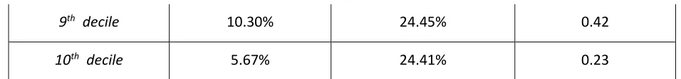
Similar changes as it comes to average return and standard deviation of returns can be observed for decile analysis.

Average return St. Deviation of returns Sharpe ratio

1st _{decile 13.28% 21.43% 0.62}

2nd _{decile 17.02% 24.52% 0.69}

3rd _{decile 16.24% 22.48% 0.72}

4th _{decile 17.14% 23.53% 0.73}

5th _{decile 15.49% 23.16% 0.67}

6th _{decile 14.88% 23.81% 0.63}

7th _{decile 14.03% 25.15% 0.56}

8th _{decile 13.02% 24.21% 0.54}

-20.00% -10.00% 0.00% 10.00% 20.00% 30.00% 40.00%

Results of analysed portfolios - US & Canada (ex. 1999 - 2004)

Page | 20

9th _{decile 10.30% 24.45% 0.42}

10th _{decile 5.67% 24.41% 0.23}

Table 10 Decomposition of returns in deciles – US & Canada (ex. 1999-2004)

The shift of Sharpe ratio curve is not parallel, but there is observable characteristic shape of curve.

Figure 5 Average key parameters for deciles in US & Canada (ex 1999-2004)

As can be seen from data presented above excluding five “exceptional” years do not change the overall results of strategy – Sharpe ratio is still relatively high comparing to other strategies.

IV. I. II US & Canada

–

monthly data

As the availability of data for US & Canadian market is satisfactory and this is the most important market also strategy in monthly intervals was analysed. Results are very satisfactory and even higher as it comes to Sharpe ratio than for US & Canada calculated yearly. This might be justified by a lower standard deviation of returns and bigger sample, which makes results more reliable.

Portfolio Average annualized return

Annualized st.

deviation of returns Sharpe ratio

% of positive results

0.00% 10.00% 20.00% 30.00% 40.00% 50.00% 60.00% 70.00% 80.00%

1st decile 2nd decile 3rd decile 4th decile 5th decile 6th decile 7th decile 8th decile 9th decile 10th decile

Average key parameters for deciles in US&Canada (ex. 1999-2004)

Page | 21

50/50 portfolio 4.98% 5.43% 0.92 64.26%

25/75 portfolio 7.57% 8.28% 0.91 63.14%

10/90 portfolio 9.20% 11.93% 0.77 64.74%

5-50/50-95

portfolio 5.41% 6.57% 0.82 65.06%

Table 11 Performance of different portfolios in US & Canada for monthly intervals

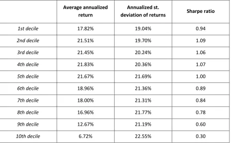
As it comes to return in deciles also characteristic shape of Sharpe curve ratio can be seen. The highest Sharpe ratio is for around 3rd _{decile and then monotonically decrease. In line with expectations.}

Average annualized return

Annualized st.

deviation of returns Sharpe ratio

1st decile 17.82% 19.04% 0.94

2nd decile 21.51% 19.70% 1.09

3rd decile 21.45% 20.24% 1.06

4th decile 21.83% 20.36% 1.07

5th decile 21.67% 21.69% 1.00

6th decile 18.96% 21.36% 0.89

7th decile 18.00% 21.31% 0.84

8th decile 16.96% 21.77% 0.78

9th decile 12.67% 21.19% 0.60

10th decile 6.72% 22.55% 0.30

Page | 22

Figure 6 Average key parameters for deciles in US & Canada – monthly interval

Figure 7 Cumulated return for LVH strategy for US & Canada – monthly intervals 1962-2014

0.00% 20.00% 40.00% 60.00% 80.00% 100.00% 120.00%

1st decile 2nd decile 3rd decile 4th decile 5th decile 6th decile 7th decile 8th decile 9th decile 10th decile

Average key parameters for deciles in US & Canada - monthly data

1962-2014

Average annualized return Annualized st. deviation of returns Sharpe ratio

-2 0 2 4 6 8 10 12 14

Page | 23

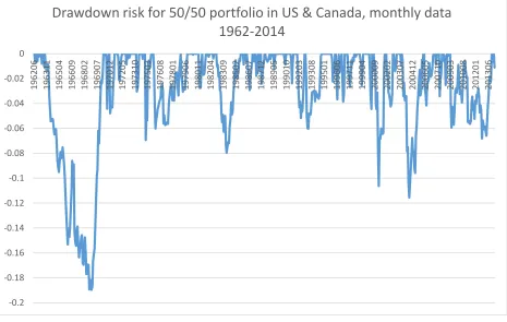
Figure 8 Drawdown risk for 50/50 portfolio in US & Canada, monthly data 1962-2014

As can be seen from figure presented above dollar-neutral strategy based on LVH factor brought around 1100% of return over the last 52 years with a maximum drawdown risk of around 19%. Moreover if we look in details tremendous growth was noticed around dot-com bubble and 2007 crisis. Although market premium factor is not statistically significant (see chapter IV.II) we can see that during a downturn on markets strategy performed OK and potential downside seems to be rather low.

IV. I. III. Europe

Analysed period of time for European companies (from developed markets) is shorter (2003-2014), which is due to a smaller availability of data (there is a need to obtain both market and financial data). This creates some risk, that results in future will be less consistent with historical ones. On the other hand analysed sample is big enough (whole backtesting universe more than 7 000 companies, with on average 2 000 companies yearly fulfilling criteria). Analysed period for Europe do not contain dot-com bubble, which as showed in previous part just a little influenced results. On the other hand analysis contains an interesting period of low interest rates, which creates opportunity for low indebted companies to leverage and gain abnormal profit.

As we can see from chart presented below net debt to EBITDA ratio, similarly like in US & Canada, is quite stable over time with median around 1. In fact this is interesting that although interest rates were lowered

-0.2 -0.18 -0.16 -0.14 -0.12 -0.1 -0.08 -0.06 -0.04 -0.02 0

196206 196311 196504 196609 196802 196907 197012 197205 197310 197503 197608 197801 197906 198011 198204 198309 198502 198607 198712 198905 199010 199203 199308 199501 199606 199711 199904 200009 200202 200307 200412 200605 200710 200903 201008 201201 201306

Drawdown risk for 50/50 portfolio in US & Canada, monthly data

Page | 24 to around 0 there is no significant increase in general level of debt. Partially this is explanation why European monetary policy is not as effective as it is in US – companies in Europe do not want to invest so much and drive domestic demand.

Figure 9 Net debt/EBITDA in analysed sample – Europe

Results obtained in Europe are even more promising than in US & Canada. Sharpe ratio for analysed portfolios was at up to 1.30, which is more than twice as much as in US & Canada. Moreover strategy almost always brought positive results.

Portfolio Average return St. Deviation of

returns Sharpe ratio

% of positive results

50/50 portfolio 9.52% 8.31% 1.15 90.91%

25/75 portfolio 15.56% 12.24% 1.27 90.91%

10/90 portfolio 20.16% 20.50% 0.98 90.91%

-3.00 -2.00 -1.00 0.00 1.00 2.00 3.00 4.00 5.00 6.00 7.00 8.00

2003 2004 2005 2006 2007 2008 2009 2010 2011 2012 2013

Net debt to EBITDA in analysed sample - Europe

Page | 25

5-50/50-95

portfolio 7.99% 6.16% 1.30 100.00%

Table 13 Performance of different portfolios in Europe

The only year, when strategy generated losses was from April 2006 to April 2007, which is in line with expectations presented In chapter II – in the last part of bull market investors who are looking for cheap companies start buying high indebted (so more risky) companies. After that when crisis begin low indebted companies perform better (due to lower risk) so strategy brings strong profits (years 2007-2009).

Figure 10 Decomposed results of analysed portfolios – Europe

While looking at results for deciles strong monotonicity is observable as it comes to average returns (from more than 30% for 1st _{decile to less than 10% for last decile). One might ask, why there is average return}

positive for every decile? There are several answers. First issue is that analysed period is from 2003, when markets were at a bottom after dot-com crisis and currently are much higher, so naturally market as a whole is up (if we look at DAX which is currently around 9000 and was around 4000 so it gives about 8% yearly return). Secondly there is natural survivorship bias while analysing historical data (hard to measure). Thirdly companies which brought negative EBITDA in one year are excluded from analysis for the next year. It might be assumed that companies which bring negative results in general give lower than market average (this is partially connected with momentum strategy). Fourthly analysed portfolios are equal weighted and not to easy comparable with the most popular market cap weighted portfolios (in Fama-French model there is size factor; in equal weighted portfolios small companies influence results stronger regardless of their level of debt – can influence both positively and negatively).

-10.00% 0.00% 10.00% 20.00% 30.00% 40.00% 50.00% 60.00% 70.00% 80.00%

2003 2004 2005 2006 2007 2008 2009 2010 2011 2012 2013

Reults of analyzed portfolios - Europe

Page | 26

Average return St. Deviation Sharpe ratio

1st _{decile 30,62% 43,99% 0,70}

2nd _{decile 28,36% 38,97% 0,73}

3rd _{decile 26,51% 31,66% 0,84}

4th _{decile 25,24% 31,45% 0,80}

5th _{decile 23,39% 33,32% 0,70}

6th _{decile 22,53% 31,00% 0,73}

7th _{decile 20,28% 30,35% 0,67}

8th _{decile 18,79% 35,79% 0,52}

9th _{decile 15,61% 32,45% 0,48}

10th _{decile 8,97% 33,54% 0,27}

Table 14 Decomposition of returns in deciles – Europe

Once again Sharpe ratio curve have a characteristic shape, with maximum around 3rd_/4th _{decile and then}

declining.

Figure 11 Average key parameters for deciles in Japan

0.00% 10.00% 20.00% 30.00% 40.00% 50.00% 60.00% 70.00% 80.00% 90.00%

1st decile 2nd decile 3rd decile 4th decile 5th decile 6th decile 7th decile 8th decile 9th decile 10th decile

Average key parameters for deciles in Europe (2003-2014)

Page | 27 Summing up, results for Europe confirms the theory that investing in low indebted companies can bring abnormal return. Moreover European example showed, that only in last part of cycle low leveraged companies underperform highly leveraged ones.

IV. I. IV. Japan

The next analysed market was Japan in years 1990 – 2014. At first the specific market and economic situation should be mentioned. Japan is a country struggling with stagflation (deflation and low growth), which is quite opposite to previously analysed markets, which makes testing hypothesis even more interesting. As we can see from chart below at first net debt/EBITDA in analysed sample was quite high, which was caused by difficult economic situation and low financial profits. In such environment thesis that low leveraged companies can use capital to takeover attractive assets and substantially increase value to current shareholders can be tested.

As can be seen with elapse of time net debt to EBITDA ratio rationalized and come with median close to 0, which is much smaller than for previously analysed markets.

Figure 12 Net debt/EBITDA in analysed sample – Japan

-10.00 0.00 10.00 20.00 30.00 40.00 50.00 60.00

Net debt to EBITDA in analysed sample - Japan

Page | 28 Average returns for presented strategy are relatively low in Japan and range from 2.68% to 8.85%, but on the other side standard deviation of returns is very low as well. Obtained Sharpe ratio ranges from 0.36 to 0.90 which is not a bad results. Also % of time when strategy brought a positive results is satisfactory.

Portfolio Average return St. Deviation of

returns Sharpe ratio

% of positive results

50/50 portfolio 3.41% 7.26% 0.47 66.67%

25/75 portfolio 6.10% 10.15% 0.60 70.83%

10/90 portfolio 8.85% 9.84% 0.90 83.33%

5-50/50-95

portfolio 2.68% 7.40% 0.36 58.33%

Table 15 Performance of different portfolios in Japan

Page | 29

Figure 13 Decomposed results of analysed portfolios – Japan

If we look on deciles, which are not a long/short strategy but decomposes results it can be seen that highly leveraged companies in 10th _{decile brought average negative return. Considering Japanese economic}

environment it should not be a surprise. Deflation makes debts larger in relative terms so it should not be

a surprise that shareholder’s wealth was transferred to creditors in highly leveraged companies.

Average return St. Deviation Sharpe ratio

1st _{decile 5,13% 28,05% 0,18}

2nd _{decile 5,66% 26,20% 0,22}

3rd _{decile 6,31% 27,10% 0,23}

4th _{decile 6,27% 25,24% 0,25}

5th _{decile 5,79% 27,01% 0,21}

6th _{decile 6,37% 29,67% 0,21}

7th _{decile 5,32% 29,22% 0,18}

8th _{decile 2,74% 26,78% 0,10}

9th _{decile 1,49% 28,79% 0,05}

-10.00% -5.00% 0.00% 5.00% 10.00% 15.00% 20.00% 25.00% 30.00% 35.00% 40.00%

Reults of analyzed portfolios - Japan

Page | 30

10th _{decile -3,76% 28,01% -0,13}

Table 16 Decomposition of returns in deciles – Japan

There is also one, even more important finding. Although Sharpe ratio is on average lower, the Sharpe ratio curve has the same shape as in previous examples with the highest value in 3rd_/4th _decile!

Figure 14 Average key parameters for deciles in Japan

Summing up, although macro situation in Japan in analysed period was quite different than for other countries the results of the strategy are similar and satisfactory as it comes to Sharpe ratio. Moreover very similar shape of Sharpe ratio curve should be emphasized.

IV. I. V. Asia & Australia

The last analysed markets are Asian (which includes Hong Kong and Singapore) and Australian (which includes Australia and New Zealand). The time period for analysis is the same like in Europe – from 2003 to 2014. Chart below presents net debt to EBITDA for analysed sample. As we can see chart is very similar to those presented for Europe. The main difference is that on average companies in Asia & Australia are a little bit less indebted (every line Is a little bit lower).

-20.00% -15.00% -10.00% -5.00% 0.00% 5.00% 10.00% 15.00% 20.00% 25.00% 30.00% 35.00%

1st decile 2nd decile 3rd decile 4th decile 5th decile 6th decile 7th decile 8th decile 9th decile 10th decile

Average key parameters for deciles in Japan (1990-2014)

Page | 31

Figure 15 Net debt/EBITDA in analysed sample – Asia & Australia

Results obtained from being long in low leveraged companies and being short in high leveraged companies are also satisfactory. Sharpe ratio for analysed portfolios ranges from 0.96 to 1.48 which is a very good result. Moreover similarly like in Europe % of positive results is very high (although numbers are the same

for every portfolio it is not true that “loss” was obtained in only one year for all portfolios).

Portfolio Average return St. Deviation of

returns Sharpe ratio

% of positive results

50/50 portfolio 11.36% 10.17% 1.12 90.91%

25/75 portfolio 13.79% 9.33% 1.48 90.91%

10/90 portfolio 13.96% 14.16% 0.99 90.91%

5-50/50-95

portfolio 10.66% 11.10% 0.96 90.91%

Table 17 Performance of different portfolios in Asia & Australia

Also in Asia & Australia typical cyclical pattern can be seen. As we can see the highest returns were gained in 2009 (which in fact embraces period from April 2009 to April 2010), which confirms the thesis presented

-4.00 -3.00 -2.00 -1.00 0.00 1.00 2.00 3.00 4.00 5.00 6.00

2003 2004 2005 2006 2007 2008 2009 2010 2011 2012 2013

Net debt to EBITDA in analyzed sample - Asia & Australia

Page | 32 in chapter II, that when crisis finishes then firstly good quality and low indebted companies brings higher rates of return.

Figure 16 Decomposed results of analysed portfolios – Asia & Australia

As it comes to decile analysis there is nothing new to be added.

Average return St. Deviation Sharpe ratio

1st _{decile 25,81% 35,45% 0,73}

2nd _{decile 29,44% 39,24% 0,75}

3rd _{decile 30,04% 39,66% 0,76}

4th _{decile 27,96% 31,47% 0,89}

5th _{decile 27,45% 38,33% 0,72}

6th _{decile 22,08% 28,82% 0,77}

7th _{decile 16,21% 27,38% 0,59}

8th _{decile 17,77% 30,31% 0,59}

9th _{decile 16,14% 31,99% 0,50}

-10.00% -5.00% 0.00% 5.00% 10.00% 15.00% 20.00% 25.00% 30.00% 35.00% 40.00% 45.00%

2003 2004 2005 2006 2007 2008 2009 2010 2011 2012 2013

Reults of analyzed portfolios - Asia & Australia

Page | 33

10th _{decile 12,43% 28,34% 0,44}

Table 18 Decomposition of returns in deciles – Asia & Australia

Again similar shape of Sharpe ratio curve can be observed, with the highest value for 4th _{decile (Sharpe}

ratio equal to 0.89).

Figure 17 Average key parameters for deciles in Asia & Australia

Summing up, results for Asia & Australia are not surprising and in line with expectations. What is interesting is similarity of results to those presented for Europe.

IV. II. Risk adjusted returns

Results presented above seems very good and natural question which should be asked is how much results presented above are related to well-known risk factors. Firstly a regression in Fama-French model was done.

𝐿𝑉𝐻 = 𝑏1∗ (𝑀𝐾𝑇 − 𝑅𝐹) + 𝑏2∗ 𝑆𝑀𝐵 + 𝑏3∗ 𝐻𝑀𝐿 + 𝑎𝑙𝑓𝑎

0.00% 10.00% 20.00% 30.00% 40.00% 50.00% 60.00% 70.00% 80.00% 90.00% 100.00%

1st decile 2nd decile 3rd decile 4th decile 5th decile 6th decile 7th decile 8th decile 9th decile 10th decile

Average key parameters for deciles in Asia & Australia (2003-2014)

Page | 34 As we can see there is no risk free rate on the right hand of equation, because LVH portfolios are dollar-neutral (which means I am regressing a factor premium against other premiums and not against long portfolio). Data to run regression were collected from Kenneth R. French website16_{. Results are presented}

below.

SUMMARY OUTPUT

Regression Statistics

Multiple R 0.54 R Square 0.30 Adjusted R

Square 0.29

Standard

Error 1.32

Observations 624

ANOVA

df SS MS F

Significance F

Regression 3 453.41 151.1382 87.0227 0.0000 Residual 620 1076.80 1.7368

Total 623 1530.21

Coefficients

Standard

Error t Stat P-value Lower 95%

Upper 95% Lower 95.0% Upper 95.0%

Intercept 0.567 0.054 10.462 0.000 0.460 0.673 0.460 0.673 Mkt-RF 0.004 0.013 0.344 0.731 -0.020 0.029 -0.020 0.029 SMB -0.138 0.018 -7.625 0.000 -0.173 -0.102 -0.173 -0.102 HML -0.295 0.020 -15.048 0.000 -0.334 -0.257 -0.334 -0.257

Table 19 Regression analysis – Fama French three-factor model

As we can see alfa (intercept) is above zero and is statistically significant, which is a very good result. Moreover SMB and HML factors are statistically relevant with negative and relatively coefficient, which can be interpreted as a fact, that using LVH in line with SMB and HML strategies can bring profits from diversification. P-value for market premium factor is statistically unimportant, which means that strategy brings good results regardless of market situation which is also a characteristics of a good strategy.

Then regression was extended to Carhart four-factor model by adding momentum factor (known as a MOM or UMD – data also from Kenneth R. French website).

Page | 35 𝐿𝑉𝐻 = 𝑏1∗ (𝑀𝐾𝑇 − 𝑅𝐹) + 𝑏2∗ 𝑆𝑀𝐵 + 𝑏3∗ 𝐻𝑀𝐿 + 𝑏4∗ 𝑀𝑂𝑀 + 𝑎𝑙𝑓𝑎

SUMMARY OUTPUT

Regression Statistics

Multiple R 0.57 R Square 0.33 Adjusted R

Square 0.32

Standard

Error 1.29

Observations 624

ANOVA

df SS MS F

Significance F

Regression 4 497.490 124.372 74.547 0.000 Residual 619 1032.721 1.668

Total 623 1530.210

Coefficients

Standard

Error t Stat

P-value Lower 95%

Upper 95%

Lower 95.0%

Upper 95.0%

Intercept 0.510 0.054 9.413 0.000 0.404 0.617 0.404 0.617 Mkt-RF 0.012 0.012 0.972 0.332 -0.012 0.036 -0.012 0.036 SMB -0.124 0.018 -6.941 0.000 -0.159 -0.089 -0.159 -0.089 HML -0.284 0.019 -14.643 0.000 -0.322 -0.246 -0.322 -0.246 MOM 0.064 0.013 5.140 0.000 0.040 0.089 0.040 0.089

Table 20 Regression analysis Carhart’s four-factor model

Adding momentum factor to regression did not bring so much difference. It should be noticed that MOM factor is statistically important with positive coefficient, which means that in order to obtain alfa for 1 unit of long LVH strategy 0.064 unit of MOM should be shorted (SMB and HML should be long 0.124 and 0.284 respectively), which is interesting because normally being long MOM factor is claimed to bring abnormal profits. Alfa in Carhart four-factor model is still positive and statistically important (and it should be noticed that alfa is around 0.51% monthly, which annualized brings a nice profit of around 6.3% yearly).

Page | 36 conducted. Data were gathered from A. Frazzini website17_{. Moreover instead of classical HML factor}

author took HML Devil factor.

𝐿𝑉𝐻 = 𝑏1∗ (𝑀𝐾𝑇 − 𝑅𝐹) + 𝑏2∗ 𝑆𝑀𝐵 + 𝑏3∗ 𝐻𝑀𝐿 𝐷𝑒𝑣𝑖𝑙 + 𝑏4∗ 𝑀𝑂𝑀 + 𝑏5∗ 𝐵𝐴𝐵 + 𝑏6∗ 𝑄𝑀𝐽 + 𝑎𝑙𝑓𝑎

SUMMARY OUTPUT

Regression Statistics

Multiple R 0.60 R Square 0.36 Adjusted R

Square 0.36

Standard

Error 1.26

Observations 624

ANOVA

df SS MS F

Significance F

Regression 6 558.291 93.049 59.070 0.000 Residual 617 971.919 1.575

Total 623 1530.210

Coefficients

Standard

Error t Stat P-value Lower 95%

Upper 95%

Lower 95.0%

Upper 95.0%

Intercept 0.640 0.056 11.444 0.000 0.530 0.750 0.530 0.750 Mkt-RF 0.002 0.014 0.161 0.872 -0.026 0.031 -0.026 0.031 SMB -0.038 0.022 -1.722 0.086 -0.082 0.005 -0.082 0.005 HML Devil -0.274 0.024 -11.62 0.000 -0.320 -0.227 -0.320 -0.227 MOM -0.048 0.019 -2.613 0.009 -0.085 -0.012 -0.085 -0.012 BAB -0.101 0.018 -5.641 0.000 -0.136 -0.066 -0.136 -0.066 QMJ 0.002 0.032 0.052 0.958 -0.061 0.064 -0.061 0.064

Table 21 Regression analysis – other factors

What is interesting adding BAB factor made SMB factor statistically significantly less important. The second finding is that momentum factor is still statistically relevant, but the sigh has changed from 0.064 to -0.048. Generally speaking as we can see above three factors are important and every of them has a negative sign, which means that good combination of them and LVH factor can bring abnormal return

Page | 37 (alfa is bigger in last regression as well). Adjusted R square is some 0.36, which is fine for financial models, nevertheless further attempts to explain returns of LVH strategy should have been done.

Moreover there is another interesting issue with factors in period 196204-201403.

196204 - 201403 LVH Mkt-RF SMB HML Devil MOM BAB QMJ

Average (monthly) 0.415 0.065 0.198 0.371 0.719 0.808 0.323

St. Deviation (monthly) 1.567 4.542 2.753 3.377 4.099 3.233 2.365

Annualized Sharpe ratio 0.918 0.050 0.250 0.380 0.608 0.866 0.473

Table 22 Basic statistics for analyzed factors

Comparing to other factors average18 _{monthly premium for analysed period is not the highest and factors}

like MOM or BAB brings significantly higher return. On the other hand monthly standard deviation in LVH factor is significantly lower, which makes higher annualized Sharpe ratio for the factor.

In my theory low leveraged companies outperform highly leveraged ones due to a possibility to borrow money at right time and significantly accelerate growth. However if general level of debt in economy is low and every company can gain additional capital there should be no abnormal gains for investing in low leveraged companies (because they cannot make us of their low net debt to EBITDA position). On the other side when general level of debt in economy is very high then low indebted companies can significantly outperform highly leveraged ones, which do not have a possibility to gain more capital.

So the factor, which might drive returns of portfolios is level of net debt to EBITDA in economy. As it is impossible to measure whole net debt to EBITDA in whole economy median net debt to EBITDA for analysed samples was taken, nevertheless due to the fact that adjusted R square was equal 0.041 hypothesis that LVH strategy is driven by median level of debt in analysed sample can be rejected.

Accordingly to informal model presented in chapter II results of LVH strategy should depends on a market cycle, but analysis presented above shows no statistical significance for market premium factor.

Page | 38

V. Findings

Presented analysis shows a strong performance of portfolios built on LVH factor. In fact it seems to be too good to be true, but analysis was conducted on several markets in a long time period and for US & Canada also in monthly intervals. Obtained results confirms the theory, that low leveraged companies can obtain higher rates of returns, which is in line with expectations. Regression analysis shows strong and statistically significant alfa. Moreover negative coefficient for other factors offers a possibility to diversify portfolio and obtain abnormal profit.

For each market characteristic shape of Sharpe ratio curve was found. The highest value of Sharpe ratio was generally found for 3rd_/4th _{decile. This might be justified by the fact, that companies from 1}st_/2nd _decile

are afraid of using debt financing even if there are favorable possibilities to expand. In such case they do not take any advantage of expansion option so rates of returns are lower.

From theoretical point of view presented results are in opposition to Modigliani – Miller model and are the further step in discussion whether structure of liabilities & equities can influence value. To my mind investing in low leveraged companies can create abnormal returns, nevertheless before practical implementation of strategy it should be checked for particular markets/sectors e.g. only for S&P 500 etc.