A Monte Carlo Simulation Approach to Forecasting Multi period Value at Risk and Expected Shortfall Using the FIGARCH skT Specification

(1)

Munich Personal RePEc Archive

A Monte Carlo Simulation Approach to

Forecasting Multi-period Value-at-Risk

and Expected Shortfall Using the

FIGARCH-skT Specification

Degiannakis, Stavros and Dent, Pamela and Floros, Christos

Department of Economics, Portsmouth Business School, University

of Portsmouth, Postgraduate Department of Business

Administration, Hellenic Open University

2014

Online at

https://mpra.ub.uni-muenchen.de/80431/

(2)

1 A Monte Carlo Simulation Approach to Forecasting Multi-period Value-at-Risk and

Expected Shortfall Using the FIGARCH-skT Specification

Stavros Degiannakis∞,*,**, Pamela Dent* and Christos Floros* *

Department of Economics, Portsmouth Business School, University of Portsmouth, Richmond Building, Portland Street, Portsmouth, UK, PO1 3DE

**

Postgraduate Department of Business Administration, Hellenic Open University, Aristotelous 18, Greece, 26 335,

Abstract

In financial literature, Value-at-Risk (VaR) and Expected Shortfall (ES) modelling is focused on producing 1-step ahead conditional variance forecasts. The present paper provides a methodological contribution to the multi-step VaR and ES forecasting through a new adaptation of the Monte Carlo simulation approach for forecasting multi-period volatility to a fractionally integrated GARCH framework for leptokurtic and asymmetrically distributed portfolio returns. Accounting for long memory within the conditional variance process with skewed Student-t (skT) conditionally distributed innovations, accurate 95% and 99% VaR and ES forecasts are calculated for multi-period time horizons. The results show that the FIGARCH-skT model has a superior multi-period VaR and ES forecasting performance.

Keywords: Expected Shortfall, FIGARCH, Forecasting, stock indices, skewed Student-t,

Volatility, Long Memory, Value-at-Risk, VaR.

JEL Classifications: G17; G15; C15; C32; C53.

(3)

2 1. Introduction

Value-at-Risk (VaR) is an important tool in risk measurement and the management of the financial assets. Originally used internally by financial institutions to assess risk, VaR assumed greater significance when the Basel Committee encouraged its use through the 1996 Market Risk Amendment to the 1988 Basel Accord (Basel, 1988; Basel, 1996). Subsequently, the Basel Committee has refined the regulations relating to the use of VaR, allowing greater flexibility for certain financial institutions to use their own internal VaR models subject to the models being approved by the regulator (Basel, 2006).

VaR quantifies the maximum loss for a portfolio of assets under normal market conditions over a given period of time and at a certain confidence level. Although financial institutions have flexibility over the model which is used to estimate VaR, the regulations prescribe that they use up to one year of historical data to calculate the daily VaR for their positions. This daily VaR should be up scaled to a 10-day VaR figure to represent the banks having at least a 10-day holding period for any given position. The recent financial crash has highlighted the importance and need for reliable models to predict VaR, and has led to further amendments to the regulations, which now require financial institutions to additionally calculate a ‘stressed value-at-risk’ measure using a one year data period in which the bank incurred significant losses (Basel, 2009). Expected Shortfall (ES) is an alternative to VaR that is more sensitive to the shape of the loss distribution in the tail of the distribution. ES quantifies the expected value of the loss, given that a VaR violation has occurred.

Within the literature the ability of a variety of increasingly complex models (both parametric and non-parametric) to estimate and forecast VaR has been tested. These models can account variously for certain features of financial asset returns such as heteroskedasticity, asymmetry or leverage effects, leptokurtic distribution and long memory (hyperbolic decline of the conditional variance); see Alexander (2008) for more details. The various competing models have been compared using a range of distributions for the standardised residuals (normal, Student-t, skewed Student-t, generalized error distribution, stable Paretian, exponential generalized beta), across a number of markets for different levels of statistical significance, often for both long and short positions; see González-Rivera et al. (2004), Xekalaki and Degiannakis (2010) for more details.

(4)

3

Furthermore, a model found to be superior for estimating VaR for long positions may not be optimal for estimating VaR for short positions due to the asymmetric distribution of financial returns (Shao et al., 2009).

The empirical success of the Generalised Autoregressive Conditional Heteroscedasticity (GARCH) framework (Engle, 1982 and Bollerslev, 1986) to model high frequency volatility has been widely highlighted, with many papers focussing on the selection of the optimal GARCH specification in order to calculate and predict VaR (see, for example, Giot and Laurent, 2003a, 2003b, 2004, Caporin, 2008, Tang and Shieh, 2006, McMillan and Kambouroudis, 2009). Literature provides evidence that among the simple models, the GARCH(1,1) model is the most adequate one. Thus, our intention is to compare the baseline model with a more complex specification to allow an assessment of the trade-off between complexity and accuracy. Berkowitz and O’Brien (2002), in order to assess the performance of the banks structural models, compare their VaR forecasts with those from a GARCH model of the banks P&L volatility. They provide evidence that the banks structural VaR models do not provide forecasts superior to a simple GARCH model of P&L volatility1.

Grané and Veiga (2008) demonstrate that long memory models outperform short memory GARCH specifications, but like the majority of VaR studies, limit their backtesting to forecasting horizon of just one trading day. By contrast, financial institutions are required by the Basel Committee to calculate the VaR of their positions for at least a 10-day holding period in order to calculate their minimum capital risk requirements (Basel, 2009). Although the Basel Committee suggest that 10-day VaR may be calculated by augmenting 1-day VaR using the square root of time rule2, Wang et al. (2011), Engle (2004) and Danielsson (2002) criticise this technique on the basis that it makes the invalid assumption that the returns are independently and identically normally distributed and that volatilities over time are constant. Danielsson and Zigrand (2006) show that the square root of time scaling rule can lead to an underestimation of market risk, especially for longer time horizons. Beltratti and Morana (1999) find for horizons of one, five and ten days, that the FIGARCH model produces similar VaR forecasts to the simpler GARCH model, when the multi-period forecasts have been constructed based on the square-root-of-time rule.

Hartz et al. (2006) employ a re-sampling technique based on the bootstrap and bias correction step to improve the multi-period VaR forecasts produced by the simple normally

1

The GARCH model, for lower VaRs, is better at predicting changes in volatility and permits comparable risk coverage with less regulatory capital.

2

(5)

4

distributed AR(1)-GARCH model. They employ another standard multi-period forecasting technique of iterating the conditional mean and conditional variance specifications, using expected values where the returns or innovations are inestimable. Brooks and Persand (2003) use a similar technique to investigate methods of evaluating multi-period volatility forecasts produced by a range of GARCH family and other linear models. By contrast, Kinateder and Wagner (2010) show that a scaling-based GARCH-LM technique produces superior VaR forecasts to a benchmark fully parametric GARCH model utilising the Drost-Nijman (1993) formula for multiday volatility forecasts, especially for the five and ten day horizons.

Multi-period VaR may be estimated using a variety of techniques, including parametric or variance-covariance approaches, non-parametric approaches (e.g. historical simulation), semi-parametric approaches (e.g. extreme value theory) and Monte Carlo simulation (Dionne et al., 2009). For example, Semenov (2009) proposes a historical simulation technique which allows the accurate estimation of 1-day and 10-day VaR figures conditional on the historical sensitivity of assets returns (within a portfolio) to various macroeconomic factors (risk factor betas) over a period of time. Dionne et al. (2009) use a Monte Carlo approach to estimate intraday VaR (IVaR) using tick-by-tick data. Employing a log ACD-ARMA-EGARCH model3, they find that the approach produces reliable estimates of intra-day risk. The model benefits from its greater informational content than IVaR estimates based on regularly spaced data, and a greater flexibility with regard to the estimation time horizon. Recently, Huang (2010) uses an iterative Monte Carlo Simulation approach to produce a reliable VaR model, which more adequately models shocks to financial markets than a simple Monte Carlo Simulation. Further, Hoogerheide and van Dijk (2010) propose a technique for forecasting multiple step ahead VaR and ES using a Bayesian approach. Using data from the S&P 500 index, they find that the 10-day ahead forecasting for a single asset has similarities with the 1-day ahead forecasting (for a portfolio of 10 assets).

The present paper presents an empirical application of forecasting 1-step, 10-step and 20-step ahead 95% and 99% VaR and ES for 10 major worldwide stock indices4. Accurate VaR and ES forecasts are calculated by considering long memory within the conditional variance process and skewed Student-t conditionally distributed innovations. The Student-t

distribution is commonly used in financial risk management (VaR models) with various

3

In full, this is a log autoregressive conditional duration –autoregressive moving average – exponential GARCH model.

4

At each point in time t, the risk forecasts for the th

(6)

5

methodologies being proposed (e.g. the two piece method by Hansen, 1994, Fernandez and Steel, 1998, Bauwens and Laurent, 2005, Azzalini and Capitanio, 2003, Zhu and Galbraith, 2010). In this paper, to fully capture not only the leptokurtosis but also the asymmetry of the portfolio returns, we incorporate the skewed version of the Student-t distribution proposed by Fernandez and Steel (1998). Further, according to Hoogerheide and van Dijk (2010), the model selection has an important effect on the numerical accuracy of the VaR and ES estimates.

The key contribution of this paper is to propose a new adaptation of the Monte Carlo simulation technique of Christoffersen (2003) for forecasting multiple step ahead VaR and ES. The present paper enables i) the incorporation of long memory in the volatility of the returns as well as ii) the utilization of skewed Student-t conditionally distributed innovations in estimating multi-period VaR and ES forecasts. At present, there are, to the best of the authors’ knowledge, no studies within the literature, which estimate multi-period VaR or ES using either a fractionally integrated volatility model or leptokurtotic and asymmetric conditional distribution of innovations. Moreover, the proposed simulation-based algorithm differs from existing methods to produce long horizon VaR, in that it estimates the time path of volatility and density function for the returns and not just scaling the tail risk (see for example Wang et al. 2011).

The results show that the FIGARCH-skT model has a superior multi-period VaR and ES forecasting performance to the GARCH-skT model, for the 10-step and 20-step ahead time horizons. The result that accounting for fractional integration and asymmetric and leptokurtic conditional distribution improve the multi-period VaR and ES forecasting performance should prove to be valuable information for risk analysts and managers.

The remainder of the paper is organised as follows: Section 2 presents the framework of the GARCH-skT and FIGARCH-skT models. Section 3 shows the methods for modelling 1-step ahead and multiple step ahead VaR and ES, while Section 4 describes our data. Section 5 presents the empirical analysis of this paper and Section 6 concludes the paper and summarises the main findings.

2. Modelling GARCH-skT and FIGARCH-skT

(7)

6

that the data generating process for the log-returns series,

 

T

t t

t T

t t

p p y

1 1 1 log

  

   

 

 _, wherept is

the closing price on trading day t, follows an ARCH process (Engle, 1982):

t t t

y   ,

t tzt, where zt ~ f



0,1,



, (1)



₁;



.

2

w I

g t

t  



_  



_ 

p

j j t j q

i i t i

t a a ₁

2 1

2 0

2   

 . (2)

Equation (2) can be rewritten with lag operators as follows:

 

2

 

2,

0 2

t t

t a a L  L



2 2



,

0 2

t t

t a L

L

L       

 (4) and covariance stationary models, where shocks to the volatility process decay exponentially, such as the GARCH

 

p,q specification, was too sharp. To solve this, Baillie et al. (1996) introduced the FIGARCH



p,d,q



process, by replacing the first difference operator from equation (4) with the fractional differencing operator





d

L



, 2

t t t

d

L a

L

L       

L



lie outside of the unit circle.

The fractional differencing operator





d

L



1 is defined as:





_





 

0 1

j j j d

L

L  where

_



_{  }



d j

j

   

  

1

 . ₍₆₎

In the FIGARCH model, 0d1 indicates that shocks to the conditional variance decay at a hyperbolic rate (Baillie et al., 1996). The FIGARCH model nests the IGARCH

 

p,q where

1



d , as well as the GARCH

 

p,q , where d0. FIGARCH processes are strictly stationary and ergodic but are not weakly stationary since the second moment is infinite.

There is substantial evidence for the presence of long memory in volatility of daily and high frequency datasets; see Baillie et al. (1996) and Kilic (2011). Corsi (2009) shows that long memory specification improves the forecasting accuracy of realized volatility significantly. Moreover, recent evidence on volatility forecasting applied to high frequency datasets shows that “the forecasting accuracy is improved when the long memory property is taken into account”; see Chortareas et al. (2011)5

.

The conditional mean is modelled using an ARMA(1,0) whilst in the conditional variance it is assumed that pq1. The fact that the values of time series are often taken to have been recorded at time intervals of one length when in fact they were recorded at time intervals of another, not necessarily regular, length is an effect known as the non-synchronous trading effect. Non-synchronous trading in the stocks making up an index induces autocorrelation in the return series. To control this Lo and MacKinlay (1988) suggested a first order autoregressive form for the returns’ process. For more details see Campbell et al. 1997. Following Angelidis et al. (2004), we do not select the order of p and

q according to a model selection criterion, such as the Akaike Information Criterion (AIC) or the Schwarz Bayesian Criterion (SBC).6 They argue that in the majority of empirical studies the order of one lag has proven to work effectively in forecasting volatility for both GARCH and ARFIMA frameworks; hence, in this study we choose to set pq1.

5

Chortareas et al. (2011) argue that the FIGARCH model performs better than GARCH model when high frequency data on euro exchange rates are considered.

6

(9)

8

Further, since financial returns data is characterised by its skewness and its excess kurtosis, the standardised residuals are distributed on a skewed Student-t distribution, in preference to the normal distribution which, has been widely shown to underestimate risk, particularly in the tails of the returns distribution (see Giot and Laurent, 2003a, 2003b; Angelidis et al., 2004; Tang and Shieh, 2006; Kuester et al., 2006).

Therefore, the overall model is an AR(1)-FIGARCH



1,d,1



with skewed Student-t

distributed innovations, utilising the density function proposed by Fernandez and Steel (1998); see also Lambert and Laurent (2000, 2001)7:









_



_{ }



_









 













  











  



, , 2 1 2 2 2 2 1 2 1 2 2 2 2 1 , ; , , ; 1 , 0 ~ , 1 1 , , 1 1 1 2 1 1 1 2 1 1 . . . 2 1 1 1 2 1 1 2 2 1 1 1 0 2 1 1 1 0                                                                                          



ms z ms z if if g m sz g g s g m sz g g s g z f g v skT z b a L j d d j d b a a z y c c c y t t t t t skT d i i t t j t t j t t t t t t t t                      (7)

where g and



are the asymmetry and tail parameters of the distribution, respectively,







 

  





1



1



2 2

2

1     

 

 g g

m     , and s g2 g2 m2 1.

3. Modelling 1-step ahead and multiple step ahead VaR and ES

VaR at a given probability level



1| , |

1 ) 1 (

|

1 t t

t t

t F

VaR_ _     _ ₍₈₎

| 1 1

1 )

1 (

|

1 |



 

 

 

 t  t t  t t

t E y y VaR

ES . (9)

The proposed algorithm has been constructed in order to provide a methodological contribution to the multi-step VaR and ES forecasting under a fractionally integrated volatility framework for leptokurtic and asymmetrically distributed portfolio returns. The key innovation of this paper is the estimation of multiple step ahead VaR and ES for the FIGARCH-skT specification. The new methodology is based on the numerical technique presented in Xekalaki and Degiannakis (2010) and has been adapted from Christoffersen (2003).

Consequently, we suggest a new adaptation of Christoffersen (2003) method, for calculating multiple VaR and ES for FIGARCH-skT, using a number of steps arising from a new algorithm.

To generate the  -step ahead VaR and ES forecasts for the AR(1)-FIGARCH



1,d,1



-skT model, set out in framework (7), we employ a Monte Carlo simulation technique. Steps .1 in the algorithm are required to produce leptokurtic and asymmetrically conditionally distributed log-returns. Since analytical expressions for the multi-period density are not available, Steps .2 and .3 are used for obtaining estimates for multiperiod VaR and ES based on the fractional differencing operator. The out-of-sample observations for each index, T~,

details, see Artzner et al. (1999). I.e, VaR is not sub-additive, which means that the VaR of an overall portfolio may be greater than the sum of the VaRs of its component parts.

9

(11)

10

are divided into T~ non-overlapping intervals of observations, with  observations in each interval.10 For each non-overlapping interval, we proceed as follows11:

Step 1.1: Generate random numbers

 

MC

i i z 1 1 , _ 

from the skewed Student-t distribution, where 000

, 5 

MC denotes the number of draws (see Note 1 in the Appendix). The pseudo-random numbers are used to compute the innovations for period t1onwards.

Step 1.2: Create the hypothetical returns of time t1, as (see Note 2 in the Appendix):

 



 



  t t t t i t t t

i z c c c y

y_,₁  ₁_| _,₁ ₀ 1 ₁  ₁ , for

i



1 ,



,

MC

. (10) The return at time t1 is generated according to the AR(1) process. The value of the error term at time t1, is simulated using the relation t ₁ t ₁_|tzi_,₁

 



 

 .

Step 1.3: Create the forecast variance for time t2 as (see Note 3 in the Appendix):

 



   









 



 



 



1





1





 



  .

2 | 1 1 2 2 | 1 1 2 | 2 2 / 1 2 1 , | 1 2 1 , | 1 1 1 0 2 2 , t t t j j t t t j t t j t t t t t i t t i t t t t t t i b a L j d d j d a z d z b a a                              



         (11)

The values of the innovations up to time t are extracted from the model's estimation, whilst the value of the innovation at time t1 is estimated, as detailed above, and is treated separately.

Step 2.1: Generate further random numbers,

 

MC

i i z 1 2 ,  

from the skewed Student-t distribution, to be used to simulate the innovations for period t2 onwards.

Step 2.2: Calculate the hypothetical returns of time t2, using the AR(1) process,

 



 



  1 , 1 1 0 2 , 2 , 2

,    1  it t t t i t i t

i z c c c y

y    , for

i



1 ,



,

MC

. (12)

Step 2.3: Create the forecast variance for time t3 as (see Note 4 in the Appendix):

 



   





















_

 



_{ }

_

_

 



_



 



  _. 1 1 1 ! 2 1 2 2 , 1 3 2 | 2 1 2 | 3 2 / 1 2 1 , 1 , 2 1 , 1 , 1 2 2 , 2 , 2 2 , 2 , 1 1 0 2 3 ,                    _               



it

t j j t t t j t t j t t t t t i t i i t i i t i i t i t t t t i b a L j d d j d a z d d z a z d z b a a                    (13)

Innovation terms relating to periods t1 onwards are simulated using the relation

.

, |t i j j t j t z       …

Repeat the process for Step3 through to Step τ-1. …

10

The use of non-overlapping intervals is necessary to avoid autocorrelation in the forecast errors.

11

(12)

11

Step τ.1: Generate further random numbers,

 

MC

i i z 1 , _ 

, from the skewed Student-t distribution, to be used to simulate the innovations for period t



onwards.

Stepτ.2: Calculate the hypothetical returns of time t



,

 



 



  1 , 1 1 0 , ,

,     1  it t t t i t i t

i z c c c y

y    . (14)

Step τ.3: Construct a density function for the returns at time t



using the 5,000 simulated

returns. Calculate the  -day



1



VaR figure for the left-hand tail of this distribution, i.e.

 



MC



i t i t t y VaR 1 , ) 1 (

| f  



     .

Repeat Steps 1.1 through to τ.3 for each of the non-overlapping intervals of  observations, such that a total of T~  VaR forecasts will be produced.

The  -day ahead ES forecast for long trading positions is the  -day ahead expected

value of the loss, given that the return at time t



falls below the corresponding value of the VaR forecast, and is defined by:







(1 )



| ) 1 ( | |          

 t  t t  t t

t E y y VaR

ES , (15)

The value of the -day ahead ES measure is given by:



(1 ~)



| ) 1 ( |      

 t  t t

t EVaR

ES , 0~. (16)

Following Dowd (2002), to calculate the ES we divide the tail of the probability distribution of returns into a large number k~ of slices each with identical probability mass, estimate the  -day ahead VaR attached to each slice and find the mean of these VaRs to estimate the  -day ahead ES12.

 







          k i k i t t t

t k VaR

ES ~ 1 ) 1 ~ 1 ( | 1 ) 1 ( | 1 ~    

 . (17)

4. Data Description

In order to examine the robustness of the VaR and ES forecasts produced by the proposed forecasting mode, VaR and ES forecasts were generated using daily returns data from 10 developed market stock indices. The indices are: Austrian Traded Index (ATXINDX), French Cotation Assistée en Continu - Continuous Assisted Quotation 40 (FRCAC40), Deutscher Aktien IndeX - Dax 30 Performance (DAXINDX), UK Financial

12

(13)

12

Times Stock Exchange 100 (FTSE100), Hang Seng (HNGKNGI), Nikkei 225 Stock Average (JAPDOWA), OMX Stockholm (SWSEALI), National Association of Securities Dealers Automated Quotations - NASDAQ 100 (NASA100), NYSE Composite (NYSEALL) and Standard and Poor’s 500 Composite (S&PCOMP). Our sample considers data from major world stock market indices with the longest continuous history13. The selection is based on the following criteria: i) the indices’ market capitalization, and ii) the fact that they are the most publicly quoted stock market indices. In addition, most indices are considered as benchmark indices for large stocks (e.g. NASDAQ, NYSE, S&P500) traded internationally as they contain about 70%-80% of the value of their individual stocks (the selected indices track the performance of large companies based in the specific country). Moreover, the list includes world’s top stock exchanges by value shares traded as reported by World Federation of Exchanges Industry Association (WFE); see www.world-exchanges.org. The data, which was obtained from Datastream® for the period from 12th January, 1989 until 12th February, 2009, was conditioned to remove any non-trading days. Thus, the total number of log returns for a given index, T, ranged from 4,924 for the Nikkei 225 Stock Average, to 5,051 for the FTSE100 Index. Based on a rolling sample of Tˆ 2,000 observations, a total of T~T Tˆ

out-of-sample forecasts were produced for each model (with the parameters of the conditional mean, conditional variance and density function re-estimated each trading day) 14.

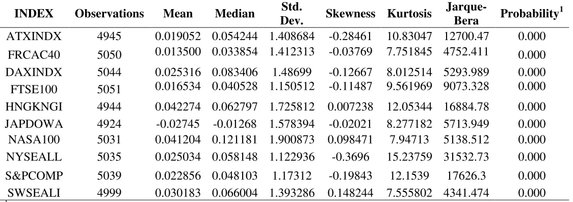
Descriptive statistics for the daily log-returns for the selected indices are given in Table 1. All of the returns distributions are leptokurtic and the majority are negatively skewed. The Jarque-Bera test results indicate that none of the log-returns series follow a Gaussian distribution. The absolute value of the log returns are significantly positively autocorrelated for a high number of lags. Examining the correlograms for the various indices, the decay in the value of the autocorrelation coefficients is initially rapid, before slowing and is suggestive of the hyperbolic decay which is typical for a long memory volatility process15.

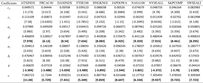
Table 2 reports the full sample parameter estimates of the FIGARCH-skT model in order to provide a fair amount of evidence that i) the long-memory of conditional volatility as well as ii) a leptokurtic and asymmetric conditional distribution of innovations are present. The long memory parameter is statistically significant for all the indices supporting the

13

For example, the Austrian ATX as well as the Swedish OMX indices are the leading indices of the Wiener

Borse and the Stockholm Stock Exchange, respectively; both are two of the world’s oldest exchanges (Wiener

Borse was founded in 1771, while Stockholm Exchange was founded in 1863).

14

The estimations were carried out using the G@RCH 6.0 (Laurent, 2009) package of Ox (Doornik, 2009).

15

(14)

13

presence of long-memory. Moreover, the parameters of the skewed Student-t distribution are statistically significant strongly supporting the use of a skewed and leptokurtic distribution.

5. Empirical Analysis

5.1. Evaluation Framework

A model is considered to accurately forecast the  -step ahead VaR if it cannot be rejected by both the independence and conditional coverage hypotheses. Potential clustering of the VaR violations is an important consideration, and is tested for using the independence hypothesis. Christoffersen (1998) examines whether the instances of VaR failure are independent, based on the likelihood ratio statistic given below:













2

1 11

11 01

01 1 2log 1 ~ ~ ~

1 log 2 11 01 10 00 11 10 01

00   

 _                        

n n n

n n n n n IN T N T N LR , (18) where, N is the number of days on which a violation occurred across the total VaR estimation period T~, nij is the number of observations with value i followed by j for

1 , 0 ,j

i , and



 j ij ij ij n n

 are the corresponding probabilities16. The purpose of the test is to

examine the null hypothesis that the VaR failures are independent and are spread over the whole estimation period, against the alternative hypothesis that the failures tend to be clustered. The main advantage of the test is that it can reject a model that generates either too many or too few clustered exemptions (see Cheng and Hung, 2010). As Angelidis et al. (2004) argue, the Christoffersen (2003) procedure can be used to separate clustering effects from distributional assumption effects.

The conditional coverage hypothesis (Christoffersen, 1998, 2003) combines Kupiec’s (1995) test with independence hypothesis, and examines the null hypothesis that the observed violation rate, N T~, is statistically equal to the expected violation rate,  as well as that the VaR failures are independently distributed over time. In order to test this null hypothesis, the likelihood ratio statistic is:









2

2 11 11 01 01 ~ 11 10 01

00 (1 )

) 1 ( log 2 ) 1 ( log

2        



 TN N n n n n

cc

LR . (19)

16 1 ,j

i indicates that a violation has occurred, whereas i,j0 indicates the converse. _ij indicates the probability that j



0,1



occurs at time t, given that i



0,1



occurred at time t1. The null hypothesis is

11 01 0: 

(15)

14

The most widely applied tests are those of Kupiec (1995) and Christoffersen (2003). However, testing for the validity of the VaR forecasts other tests have also been considered, i.e. density forecasts test of Berkowitz (2001), CAViaR test of Engle and Manganelli (2004), and they provide qualitatively similar results.

If the null hypothesis of both the independence and conditional hypotheses is not rejected for a particular model, then we conclude that the model produces the expected proportion of VaR violations, and that these violations are not clustered together.

However, it does not provide a method for distinguishing between the performances of the various models for which this is the case. Sarma et al. (2003) and Angelidis and Degiannakis (2007) suggest a two-stage backtesting procedure. In the first stage, the VaR forecasting ability of the candidate models is investigated, and in the second stage the forecasting accuracy of the models, which are judged to forecast the VaR adequately in the first stage, is compared. For the present study, in the first stage, the VaR forecasting ability of the candidate models is investigated according to the likelihood ration statistics in (18) and (19). For the second stage, the mean squared error, or MSET



t

1

~

, is calculated for the loss function:

 





  

 _ _

    



. 0

, VaR

y (1 |)

2 1

| t

otherwise y if

ESt t t t t

t

  



 (20)

Therefore, we pick risk models that calculate the VaR accurately, as the prerequisite of independence and correct conditional coverage is satisfied, and provide more precise ES forecasts, as they minimize the MSE. The MSE evaluates the  -day ahead ES forecasts. Thus for each VaR failure we compare the actual return to the forecasted return, given that the VaR is violated. Hence, the model will be deemed to perform well if:

i) the VaR failures occur independently of each other (Christoffersen, 1998 test);

ii) the observed failure rate equals the expected failure rate (Christoffersen, 1998, 2003 test);

iii) the MSE based on the quadratic loss between the actual and expected returns in the event of a VaR violation is minimised (Hansen, 2005 test).

Finally, we should check whether the MSE values of the models differ statistically significant. Hansen (2005) proposed the Superior Predictive Ability, or SPA, test for comparing the performances of two or more forecasting models in terms of a predefined loss function, t . Let us denote as

 A t 

 _ and  B t 

(16)

15

and GARCH-skT models, respectively. The null hypothesis that the FIGARCH-skT model is not outperformed by the GARCH-skT model, or ₀ :



 _   _B



0

t A t

E

H  _  _ , is tested against the alternative, ₁ :



   t B



0

A t

E

H     .17 Obviously, the t A and

 B t 

 _ may be considered for various modifications of the loss function, i.e. the absolute distance, (1 )

|

ES p t t t

y__  __ , as well as the absolute percentage distance,



_  _



t_

) 1 (

| y

ES p t t t

y .

5.2. Empirical Results

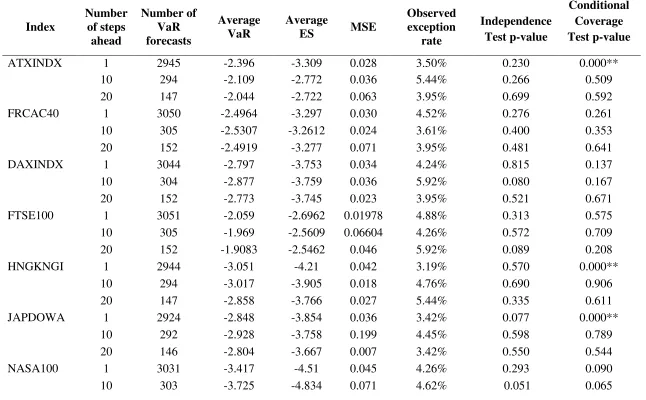
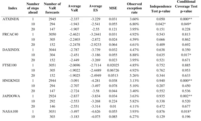
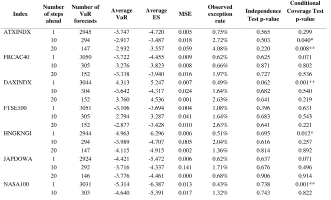
The empirical results for forecasting 1-step, 10-step and 20-step ahead 95% VaR using the FIGARCH and GARCH models based on skewed Student-t distribution are shown in Tables 3 and 4, respectively. According to the conditional coverage test, the FIGARCH-skT model produces an adequate forecasting performance for 5, 10 and 10 indices (out of the 10 indices tested) at the 1-step ahead, 10-step ahead and 20-step ahead forecasting horizons, respectively. This compares favourably to the GARCH-skT model which produces an adequate forecasting performance for 4, 8 and 10 indices (out of the 10 indices tested) at the 1-step ahead, 10-step ahead and 20-step ahead forecasting horizons, respectively. Accounting for fractional integration in the volatility model improves the adequacy of the 95% VaR forecasts at the 10-step horizon, for which the FIGARCH-skT model adequately predicts losses for all the 10 indices.

For the FIGARCH-skT model, the results of the independence test indicate that the null hypothesis that the VaR violations occur independently cannot be rejected for any of the indices for any time horizon. Similarly, for the GARCH model, the null hypothesis of independence between the VaR violations cannot be rejected for any of the indices at any time horizon except for the ATXINDX at the 10-step ahead time period. Thus, the FIGARCH-skT and GARCH-skT specifications demonstrate a comparable performance in terms of the independence of the VaR violations, in the multi-period VaR forecasts.

Furthermore, the average 95% ES figure tends to decrease as the forecasting horizon increases for the FIGARCH-skT model across all of the indices. By contrast, the average 95% ES figure for the GARCH-skT model decreases between the 1-step and 10-step ahead

17

The SPA statistic equals to



   





   



2 / 1 /

~

1 1 /

~

1

1 ~

~ 

  



  



    

  

   

 

 





  



    



 T

t

B t A t T

t

B t A

t V T

T

(17)

16

forecasting horizons for all of the indices, but, subsequently, increases between the 10-step and 20-step ahead forecasting horizons. The MSE of the ES figures for the FIGARCH-skT model are generally lower than those for the GARCH-skT model, especially as the forecasting horizon increases. For example, the MSE of the 1-step ahead 95% ES figures are greater for the FIGARCH-skT model than the GARCH-skT model for 5 of the 10 indices. However, the MSE of the 10-step ahead ES figures for the FIGARCH-skT model are lower than, or equal to, those for the GARCH-skT model for all 10 indices. Furthermore, the MSE

of the 20-step ahead ES figures are lower for the FIskT model than the GARCH-skT model for 8 of the 10 indices.

In order to evaluate the performance of the models, we proceed to the statistical comparison of the mean squared error loss function in (20). Table 5 presents the p-values of the SPA test for the null hypothesis that the FIskT model outperforms the GARCH-skT model. A high p-value indicates evidence in support of the hypothesis that the FIGARCH-skT model is superior to the GARCH-skT. As all the p-values of the SPA test are greater than 0.05, there is evidence suggesting that the FIGARCH-skT model does not demonstrate an inferior performance to the GARCH-skT model in forecasting losses when the VaR figure is breached. In the second part of Table 5, the mean absolute error loss function is applied, which provides qualitatively similar results18. We, therefore, conclude that the FIGARCH-skT model does demonstrate a superior performance to the GARCH-skT model in forecasting multiple step ahead losses.

The empirical results for forecasting 1-step, 10-step and 20-step ahead 99% VaR using the FIGARCH and GARCH models based on skewed Student-t distribution are shown in Tables 6 and 7, respectively. The results are qualitatively similar to the 95% case; the fractional integration in the volatility model improves the adequacy of the 99% VaR forecasts at the 10-step and 20-step horizons. The conditional coverage test informs us that the FIGARCH-skT model produces adequate forecasting performance for all the 10 indices at the 10-step ahead and 20-step ahead forecasting horizons. This compares favourably to the GARCH-skT model which produces an adequate forecasting performance for 8 and 9 indices (out of the 10 indices tested) at the 10-step ahead and 20-step ahead forecasting horizons, respectively. On the contrary, both models fail to fulfil the conditional coverage for the next

18

The  A t 

 and

 B t 

 have been computed for

 

  

 

 

  

1 | t

y t t

t ES if

) 1 (

|

VaR  

    t t t

y and t 0otherwise.

(18)

17

trading day; in 8(5) out of the 10 indices the FIGARCH(GARCH) model does not produce an adequate forecasting performance at the 1-step ahead time horizon.

The MSE of the 10-step ahead 99% ES figures for the FIGARCH-skT model are lower than those for the GARCH-skT model for 9 out of the 10 indices. As in the case of 95% confidence interval, the evaluation of the performance of the models with the SPA test provide evidence in support of a superior performance to the GARCH-skT model in forecasting multiple step ahead losses19.

The magnitude of the observed failure rate for each forecasting horizon suggests that both models tend to over-forecast the VaR figure at the 1-step ahead time horizon, but that this tendency diminishes for longer forecasting horizons, and in particular for the 10-step ahead forecasting horizon. This contrasts with the findings of Kuester et al. (2006) who found that VaR models tend to underestimate the true VaR figure for the 1-step ahead time horizon. It is interesting to compare the volatility of the returns. Figures 1 and 2 show plots for observed returns against the 95% VaR forecasts resulting from the FIGARCH-skT and GARCH-skT models for the SWSEALI and HNGKNGI indices for the 1-step, 10-step and 20-step ahead forecasting horizons20. Looking at the plots for the SWSEALI index (Figure 1a), it appears that although the most recent returns (representing the start of the global financial crisis) are quite volatile in the 1-step 95% VaR plot, the graph (Figure 1b) showing every 10th return (for the 10-step VaR forecasts) displays less volatility. Comparing this to the plots for the HNGKNGI index (Figure 2), which is slightly more volatile, when we consider all the returns, than the SWSEALI index, but is much more volatile when we consider every 10th return figure (for the 10-step VaR forecasts). The proposed method performs particularly well for the SWSEALI index.

5.3. Square-root Rule

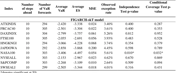
As noted by Danielsson and Zigrand (2006) and Engle (2004), the square root of time scaling rule appears to lead to inadequate VaR forecasts and, hence, the objective of the Basle Committee is not addressed satisfactorily. Table 8 reports the forecasting 10-day-ahead 95%

19

The p-values of the SPA test are available to the readers upon request.

20

(19)

18

VaR and 95% ES using the FIGARCH-skT model based on the square root rule21. According to the independence and conditional coverage tests, at the 10-step ahead forecast, the square of root rule does not produce adequate risk forecasts for just 1 out of the 10 indices. Even the square-root rule under an appropriate modelling framework is able to provide proper risk forecasts. However, the comparison of the square-root rule to the FIGARCH-skT model under the Monte Carlo simulation technique is in favour of the proposed method. There is significant difference of the percentage of observed violations between the square-root rule (in Table 8) and the proposed simulation technique. For 9 out of the 10 indices, the observed exception rate is closer to 5% for the proposed simulation technique compared to the square-root rule (for the DAXINDX the absolute difference of observed exception rate from 5% is 0.26% under the square-root rule and 0.92% under the proposed simulation technique).

Therefore, we provide a further support that the proposed multi-period forecasting risk method is not just a byproduct of a shift in the unconditional variance but instead it does capture the long-memory of volatility. Hence, our findings are in accordance with Danielsson and Zigrand (2006); "even if the square root of time rule has widespread applications in the Basel Accords, it fails to address the objective of the Accords".

6. Conclusion and Suggestions for Further Research

This paper has introduced a new adaptation to the FIGARCH-skT model of the Monte Carlo simulation technique of Christoffersen (2003) for forecasting multiple step ahead 95% and 99% VaR and ES. Much of the existing literature on VaR forecasting is limited to the 1-step ahead horizon, or employs unjustifiable assumptions to produce multiple 1-step ahead forecasts using scaling rules such as the square root of time rule.

The VaR forecasting accuracy of the simulation technique was tested on 10 worldwide stock indices. Based on a two-stage backtesting procedure, the VaR forecasting ability of the candidate models is investigated, and the forecasting accuracy of the models, which are judged to forecast the VaR adequately, is compared. The Superior Predictive Ability test compares the forecasting performance of the competing models in terms of a predefined loss function.The results show that the FIGARCH-skT model has a superior 95% and 99% VaR and ES forecasting performance to the GARCH-skT model, for the 10-step and

21

The square-root rule assumes that  -day ahead variance forecasts are equal for each day  . Therefore, under the square-root rule, the 10-day ahead VaR is constructed as



 t



_t _t

t t t

t F

VaR 1| 1|

%) 95 (

|

10  ; 

(20)

19

20-step ahead time horizon. Furthermore, the tendency for the models to over predict the VaR figure for the 1-step ahead horizon, appeared to diminish for longer forecasting intervals.

The Basel regulations require a 10-day VaR. The FIGARCH-skT model performs accurately at the 10-day and 20-day ahead 95% and 99% VaR. Is there anything in the structure of the model or the nature of the markets that may cause this to happen? For the 1-day horizon, the long memory structured model does not perform better that the short memory. For the 10-day horizon, the FIGARCH-skT model appeared to produce its best forecasts, providing evidence that the superiority of the long memory volatility modelling is detected in two-weeks (in calendar time) forecasts, as the Basel regulations require. Although, the 20-trading-day (or the one-month in calendar time) horizon is considered a faraway point in time to be predicted, the FIGARCH-skT model provides accurate 95% and 99% VaR forecasts. However, for the 20-day time horizon, the results of the conditional coverage tests were highly sensitive to the number of VaR violations such that a very small number of additional (or fewer) violations can be pivotal in determining whether or not the forecasting performance of the model is deemed to be adequate.

Considering the case of ES forecasting, the FIGARCH-skT model does demonstrate a superior performance to the GARCH-skT model in forecasting losses given that a VaR violation has occurred. The 10-step ahead quadratic loss between the actual and expected returns in the event of a 95% VaR violation is lower for the long memory volatility model for all 10 indices. The 10-step ahead MSE in the event of a 99% VaR violation is lower for the long memory volatility model for 9 indices. Furthermore, the 20-step ahead loss function for the FIGARCH-skT model is lower for 9 of the 10 indices. Since the findings suggest that FIGARCH-skT models have a superior 95% and 99% VaR and ES forecasting performance, for the 10-step and 20-step ahead time horizons, risk managers and analysts should apply our technique to obtain accurate 95% and 99% risk forecasts.

(21)

20

nonlinear, and regime-switching dynamics (see Haas et al., 2004 and Huang, 2011), may also be investigated in future research.

Acknowledgement

Dr. Stavros Degiannakis and Dr. Christos Floros acknowledge the support from the European Community’s Seventh Framework Programme (FP7-PEOPLE-IEF) funded under grant agreement no. PIEF-GA-2009-237022.

References

Alexander, C. 2008. Value-at-Risk Models. New York: John Wiley & Sons, Inc.

Angelidis, T. and S. Degiannakis. 2007. Backtesting VaR Models: A Two-Stage Procedure.

Journal of Risk Model Validation 1: 2: 1-22.

Angelidis, T., A. Benos and S. Degiannakis. 2004. The use of GARCH models in VaR estimation. Statistical Methodology 1:105-128.

Artzner, P., F. Delbaen, J. Eber and D. Heath. 1999. Coherent Measures of Risk.

Mathematical Finance, 9: 3: 203-228.

Azzalini, A. and A. Capitanio. 2003. Distributions generated by perturbation of symmetry with emphasis on a multivariate skew t distribution, Journal of the Royal Statistical Society B 65: 2: 367–389.

Baillie, R., T. Bollerslev and H. Mikkelsen. 1996. Fractionally integrated generalised autoregressive conditional heteroscedasticity. Journal of Econometrics 74: 1: 3-30. Basel Committee on Banking Supervision. 1988. International Convergence of Capital

Measurement and Capital Standards. Basel.

Basel Committee on Banking Supervision. 1996. Amendment to the Capital Accord to incorporate Market Risks. Basel.

Basel Committee on Banking Supervision. 2006. International Convergence of Capital Measurement and Capital Standards – A Revised Framework. Basel.

Basel Committee on Banking Supervision. 2009. Revisions to the Basel II Market Risk Framework. Basel.

Bauwens, L. and S. Laurent. 2005. A new class of multivariate skew densities, with application to GARCH models. Journal of Business and Economic Statistics 23: 346– 354.

(22)

21

Berkowitz, J. 2001. Testing Density Forecasts, with Applications to Risk Management.

Journal of Business and Economic Statistics, 19: 465-474.

Berkowitz, J. and J. O’Brien. 2002. How Accurate Are Value-at-Risk Models at commercial Banks? The Journal of Finance, 57: 1093–1111.

Bollerslev, T. 1986. Generalised autoregressive conditional heteroscedasticity. Journal of Econometrics 31: 3: 307-327.

Brooks, C. and G. Persand. 2003. Volatility Forecasting for Risk Management. Journal of Forecasting 22: 1: 1-22.

Campbell, J., A. Lo and A.C. MacKinlay. 1997. The Econometrics of Financial Markets. New Jersey: Princeton University Press.

Caporin, M. 2008. Evaluating Value-at-Risk measures in presence of long memory conditional volatility, Journal of Risk 10: 3: 79-110.

Cheng, W.H. and J.C. Hung. 2010. Skewness and leptokurtosis in GARCH-typed VaR estimation of petroleum and metal asset returns. Journal of Empirical Finance 18: 1: 160-173.

Chortareas, G., Y. Jiang and J. Nankervis. 2011. Forecasting exchange rate volatility using high-frequency data: is the euro different? International Journal of Forecasting 27: 1089–1107.

Christoffersen, P. 1998. Evaluating interval forecasts. International Economic Review, 39: 841-862.

Christoffersen, P. 2003. Elements of Financial Risk Management. USA: Elsevier Science. Corsi, F. 2009. A simple approximate long-memory model of realized volatility. Journal of

Financial Econometrics 7: 2: 174–196.

Crouhy, M., D. Galai and R. Mark. 2001. Risk Management.New York: McGraw-Hill. Danielsson, J. 2002. The emperor has no clothes: Limits to risk modelling. Journal of

Banking and Finance 26: 7: 1273-1296.

Daníelsson, J. and J.P. Zigrand. 2006. On time-scaling of risk and the square root-of-time-rule. Journal of Banking and Finance 30: 10: 2701–2713.

Davidson, J. 2004. Moment and Memory Properties of Linear Conditional Heteroscedasticity Models, and a New Model. Journal of Business and Economic Statistics, 22: 1: 16-29. Degiannakis, S. and E. Xekalaki. 2007. Assessing the Performance of a Prediction Error

(23)

22

Dionne, G., P. Duchesne and M. Pacurar. 2009. Intraday Value at Risk (IVaR) using tick-by-tick data with application to the Toronto Stock Exchange. Journal of Empirical Finance 16:777-792.

Doornik, J.A. 2009. Ox: Object Oriented Matrix Programming, 6.0. London: Timberlake Consultants Press.

Dowd, K. 2002. Measuring Market Risk. New York: John Wiley & Sons, Inc.

Drost, F.C. and T.E. Nijman. 1993. Temporal aggregation of GARCH processes.

Econometrica 61: 909-927.

Engle, R.F. 1982. Autoregressive conditional heteroskedasticity with estimates of the variance of UK inflation. Econometrica 50: 987-1008.

Engle, R.F. 2004. Risk and Volatility: Econometric Models and Financial Practice. The American Economic Review 94: 3: 405-420.

Engle, R.F. and S. Manganelli. 2004. CAViaR: Conditional Autoregressive Value at Risk by Regression Quantiles. Journal of Business and Economic Statistics 22: 4: 367-381. Fernandez, C. and M.F.J. Steel. 1998. On Bayesian modelling of fat tails and skewness,

Journal of the American Statistical Association 93: 359–371.

Giot, P. and S. Laurent. 2003a. Value-at-Risk for Long and Short Trading Positions. Journal of Applied Econometrics 18: 6: 641-663.

Giot, P. and S. Laurent. 2003b. Market risk in commodity markets: a VaR approach. Energy Economics 25: 5: 435-457.

Giot, P. and S. Laurent. 2004. Modelling daily Value-at-Risk using realised volatility and ARCH type models. Journal of Empirical Finance 11: 3: 379-398.

González-Rivera, G., T.H. Lee and S. Mishra. 2004. Forecasting volatility: a reality check based on option pricing, utility function, value-at-risk, and predictive likelihood.

International Journal of Forecasting 20: 629-645.

Grané, A. and H. Veiga. 2008. Accurate minimum capital risk requirements: a comparison of several approaches. Journal of Banking and Finance 32: 11: 2482–2492.

Haas, M., S. Mittnik, and M.S. Paolella. 2004. A new approach to Markov-switching GARCH models. Journal of Financial Econometrics 2: 493–530.

Hansen, B.E. 1994. Autoregressive conditional density estimation. International Economic Review 35: 705–730.

(24)

23

Hartz, C., S. Mittnik and M. Paolella. 2006. Accurate value-at-risk forecasting based on the normal-GARCH model. Computational Statistics and Data Analysis 51: 4: 2295-2312. Hoogerheide, L. and H.K. van Dijk. 2010. Bayesian forecasting of Value at Risk and

Expected Shortfall using adaptive importance sampling. International Journal of Forecasting 26: 231-247.

Huang, A. 2010. An optimization process in Value-at-Risk estimation. Review of Financial Economics 19: 3: 109-116.

Huang, A. 2011. Volatility modeling by asymmetrical quadratic effect with diminishing marginal impact. Computational Economics 37: 301-330.

Kilic, R. 2011. Long memory and nonlinearity in conditional variances: A smooth transition FIGARCH model. Journal of Empirical Finance 18: 2: 368-378.

Kinateder, H. and N. Wagner. 2010. Market Risk Prediction under Long Memory: When VaR is higher than expected. Passau University, Working Paper.

Kuester, K., S. Mittnik and M.S. Paolella. 2006. Value-at-Risk prediction: a comparison of alternative strategies. Journal of Financial Econometrics 4: 1: 53-89.

Kupiec, P. 1995. Techniques for verifying the accuracy of risk measurement models. Journal of Derivatives 3: 2: 73-84.

Laurent, S. 2009. G@RCH 6, Estimating and Forecasting ARCH Models. London: Timberlake Consultants Press.

Lambert, P. and S. Laurent. 2000. Modeling Skewness Dynamics in Series of Financial Data. Discussion Paper, Institut de Statistique, Louvain-la-Neuve.

Lambert, P. and S. Laurent. 2001. Modeling Financial Time Series Using GARCH-Type Models and a Skewed Student Density.Universite de Liege, Mimeo.

Lo, A. and A.C. MacKinlay. 1988. Stock Market Prices Do Not Follow Random Walks: Evidence from a Simple Specification Test. Review of Financial Studies 1: 41-66. McMillan, D. and D. Kambouroudis. 2009. Are Riskmetrics forecasts good enough?

Evidence from 31 stock markets. International Review of Financial Analysis 18: 3: 117-124.

Sarma, M., S., Thomas and A., Shah. 2003. Selection of VaR models. Journal of Forecasting

22: 4: 337-358.

Semenov, A. 2009. Risk factor beta conditional Value-at-Risk. Journal of Forecasting 28: 6: 549-558.

(25)

24

Tang, T. and S. Shieh. 2006. Long memory in stock index futures markets: A value-at-risk approach. Physica A 366: 437-448.

Tse, Y.K. 1998. The Conditional Heteroskedasticity of the Yen-Dollar Exchange Rate.

Journal of Applied Econometrics 193: 49-55.

Wang, J., J. Yeh and N. Cheng. 2011. How accurate is the square-root-of-time rule in scaling tail risk: A global study. Journal of Banking and Finance 35: 1158-1169.

Xekalaki, E. and S. Degiannakis. 2010. ARCH Models for Financial Applications. New York: John Wiley & Sons, Inc.

Zhu, D. and J.W. Galbraith. 2010. A generalized asymmetric Student-t distribution with application to financial econometrics. Journal of Econometrics 157: 2: 297-305.

Appendix

Note 1: We define the scheme follows in order to create random draws from the skewed

Student-t distribution based on Lambert and Laurent (2001).

1. Generate random numbers

 

i _iMC1 from the standard uniform distribution, where

MCdenotes the number of draws22. 2. For each i compute the zi,1



random draw as23:

 





 





 





2 2 2 1 2 1 1 1 1 1 1 1 ; 1 2 1 ; 1 2 , ; g g if if s m g gF s m g F g g F i i i T i T i skT                      _         _             

 , (A1)

where F T1