External terms of trade and labor market imperfections in developing countries: theory and evidence

External terms-of-trade and labor

market imperfections in developing

countries: theory and evidence

Chaudhuri, Sarbajit and Biswas, Anindya

Dept. of Economics, University of Calcutta, Dept. of Economics,

Spring Hill College, USA

9 October 2014

External Terms-of-Trade and Labor Market Imperfections in

Developing Countries: Theory and Evidence

Sarbajit Chaudhuri

Dept. of Economics University of Calcutta

Kolkata, India

sarbajitch@yahoo.com

Anindya Biswas♠♠♠♠ Spring Hill College

Mobile, AL, USA

abiswas@shc.edu

(October 9, 2014)

ABSTRACT: The paper addresses the question of whether developing countries possess

any built-in mechanism that can cope with external terms-of-trade (TOT) shocks. Using a two-sector, full-employment general equilibrium model with endogenous labor market distortion theoretically it shows that such countries possess an inherent shock-absorbing mechanism that stems from their peculiar institutional characteristics and can lessen the gravity of detrimental welfare consequence of exogenous TOT movements. This result has been found to be empirically valid based on a panel dataset of 13 countries from 2000-2012. Our analyses lead to recommendation of an important policy that should be adhered to preserve this in-built system.

Keywords: Terms-of-trade shocks, Labor market imperfection, Welfare, Developing

countries, Panel Data.

JEL Classification: D59, D60, F41, F13, J42, J52.

♠

External Terms-of-Trade and Labor Market Imperfections in

Developing Countries: Theory and Evidence

1. Introduction and motivation

In the literature on trade and development, a very large numbers of empirical studies have pointed out that developing countries are much more vulnerable to external terms-of-trade (TOT) shocks vis-à-vis the developed nations. These fluctuations are undesirable because they contribute to significantly increased volatility in the growth of output and hence social welfare. Studies e.g. Baxter and Kouparitsas (2006), Broda (2004), Mendoza (1995) and Kose (2002) have found that TOT fluctuations are twice as large in developing countries as in developed nations. According to them the nature of composition of export baskets, high degree of trade openness and very little influence over international commodity prices have been the main responsible factors.

For minimizing the adverse effects of unfavorable TOT movements studies like Hoffmann (2007), Tornell and Velasco (2000), Broda (2004), Broda and Tille (2003), Mendoza (1995) and

Then, we have conducted a quantitative assessment of the theoretical result based on an annual panel dataset of 13 small developing countries over the recent time period of 2000-2012. In terms of economic growth, this empirical analysis finds that developing nations with higher intersectoral wage differential have been less affected during the liberalized regime vis-à-vis some other developing countries with relatively lower wage dispersion. More specifically, we have established that TOT movements in either direction have caused smaller fluctuations in per capita GDP growth in the economies with larger wage dispersion vis-à-vis the other group of countries in the post-reform period. Quite a large number of empirical studies involving consequences of TOT changes on the developing economies are available in the literature on trade and development. However, there has been virtually no work that relates welfare outcomes of external price movements to labor market institutions of the southern countries and builds up a formal theoretical structure with empirical validation. Here lies the importance of this study.

2. The theoretical analysis and results

We consider a 2×2 full-employment model with labor market imperfection in sector 2 for a small open economy. In sector 2 (a formal sector) workers receive the endogenously determined unionized wage,W*, while their counterparts in sector 1 (an informal sector) receive the competitive wage, W . There is perfect mobility of capital between the two sectors and its economy-wide return is r. All other standard assumptions of the Heckscher-Ohlin-Samuelson (HOS) model continue to hold. Sectors 1 and 2 are the export and import-competing sectors, respectively. Commodity prices,P_is are given by the small open economy assumption. Factor endowments are also exogenously given. Finally, commodity 1 is taken to be the numeraire.

directly borrow the simple unionized wage function as derived in detail in Chaudhuri and Mukhopadyay (2009) which is as follows.

2

* * ( , , )

W =W P W U ; with

2

* * *

( W ), ( W ), ( W ) 0

U W P

∂ ∂ ∂

>

∂ ∂ ∂ (1)

In equation (1) the parameter, Udenotes the bargaining strength of the labor union in

each formal sector firm.1 Besides, ( * ) 0 *

W W

E

W _{W W}

∂ = > ∂ ; 2 2 *

( ) 0

* P W E

P _{P W}

∂

= >

∂ ; and,

*

( ) 0

*

W U

E

U _{U W}

∂

= >

∂ denote the elasticities ofW* (.)with respect toW P, 2andU,

respectively; and, (E_W +E_P) 1= . 2

The equations of the general equilibrium structure of the economy are as follows.

1 1 1

L K

Wa +ra = (2)

2 2 2 2

* ( , , ) _{L K}

W P W U a +ra =P (3)

1 1 2 2

K K

a X +a X =K (4)

1 1 2 2

L L

a X +a X =L (5)

where a_ji is the amount of the jth factor required to produce one unit of output of sector

ifor j=L K, ; and,i=1, 2. Equations (2) and (3) are the two competitive zero-profit conditions for the two sectors while equations (4) and (5) are the two full-employment conditions for capital and labor, respectively. Determination of factor prices and output levels are well-known.

1

One of the most important objectives of the labor unions is to bargain with their respective employers so as to set the unionized wage,W* as much higher as possible above their reservation wage i.e. the informal sector wage,W. The higher their bargaining power,Uthe larger would be the intersectoral wage differential. However, U

is amenable to policy measures. If the government undertakes different labor market regulatory measures e.g. partial or complete ban on resorting to strikes by the trade unions, reformation of employment security laws to curb union power, Utakes a lower value.

2

It is assumed that sector 1 is more (less) labor-intensive (capital-intensive) than sector 2

in value sense i.e. 1 2

1 2

*

L L

K K

Wa W a

a > a . AsW*>W it automatically follows that sector 1 is

more (less) labor-intensive (capital-intensive) than sector 2 in physical sense.

The demand side of the model is represented as follows.

Let V denote social welfare that depends on the consumption of two commodities, denoted D₁ andD₂. The strictly quasi-concave social welfare function is depicted by

1 2

( , )

V =V D D (6)

The balance of trade equilibrium requires that

1 2 2 1 2 2

D +P D =X +P X (7)

The volume of import of commodity 2, denotedM is given by the following.

2( , )2 2

(-)(+)

M =D P Y −X

(8)

In equation (8), Ydenotes national income at domestic/international prices and is given by

1 2 2

Y =X +P X (9)

2.1 Theoretical results -- consequences of deterioration in TOT

Deterioration in TOT in the existing structure means an increase in the relative international price of commodity 2 i.e.P₂.

Totally, differentiating equations (1) – (5), the following proposition can be easily proved.

Proposition 1: Deterioration in the TOT leads to: (i) a decrease in the competitive wage,

wage, W*; (iv) decreases in wage-rental ratios,(W r/ )and(W* / )r ; (v) an increase in intersectoral wage differential, (W*−W); (v) an expansion (a contraction) of sector 2 (sector 1); and, (vi) an increase in employment of labor in sector 2, L₂(=a X_{L2 2}).

We verbally explain proposition 1 as follows. AsP₂ rises a Stolper-Samuelson effect takes

place that lowers Wand raises ras sector 2 (sector 1) is capital-intensive (labor-intensive). W* gets affected due to two reasons. An increase inP2 produces a direct

positive effect on W*(∵ 0

P

E > ) while the decrease in Wproduces an induced negative

effect (∵ E_W >0). The net effect on W*is, however, ambiguous. It depends on the

magnitudes of different technological, institutional, and trade-related parameters. Nevertheless, even if the net effect on W*is negative it would be less severe than that on

Wdue to the presence of the additional direct positive effect on the former. Consequently, the (W*−W)gap widens. However, it can be easily shown that the

(W* / )r ratio surely decreases.3 Consequently, producers in both the sectors substitute capital by labor that raises the labor-output ratios, a_L1anda_L2and lowers capital-output

ratios, a_K1 anda_K2. A Rybczynski type effect takes place leading to a contraction (an

expansion) of sector 1 (sector 2).4 As sector 2 expands, the aggregate employment of labor in this sector, L₂(=a X_{L2 2}) also increases.

We now investigate the welfare consequence of the TOT changes. Differentiating equations (1) – (9) the following expression can be derived.5

3

Mathematical proofs are quite straightforward.

4

It is needless to point out that a Stolper-Samuelson effect is followed by a Rybczynski type effect

if technologies of production are of variable-coefficient type.

5

2

1 2 2

1

( ) ( * )( )

(+) (+) (+) dL dV

W W M

V dP = − dP −

(10)

From equation (10) the following proposition readily follows.

Proposition 2: The presence of labor market imperfection, reflected in intersectoral wage

differential, can soften the blow of an exogenous TOT shock on welfare.

Proposition 2 can intuitively be explained in the following fashion. In the existing set-up

an exogenous TOT shock can affect social welfare in two ways. First, as the relative price

of the import good rises, the import-competing sector (sector 2) expands following a

Rybczynski type effect at the cost of the export sector (sector 1). As the high wage-paying

sector (sector 2) now absorbs more workers than previously the aggregate wage income

rises. This we call the labor reallocation effect (LRE), which produces a positive effect

on welfare. On the contrary, welfare deteriorates because the economy has now to pay

more for importing a certain amount of commodity 2 from the international market

whose relative price has increased. This may be termed as the value of import effect

(VIE). The magnitudes of LRE and VIE are captured by the first and second terms of the

right-hand-side of equation (10), respectively. Therefore, we find that social welfare

improves due to positive LRE and worsens due to negative VIE. So, even if the positive

LRE cannot outweigh the negative effect of VIE, it definitely neutralizes at least a part of

the aggregate detrimental outcome of the latter effect on social welfare.

The degree of labor market distortion which is reflected in the magnitude of intersectoral

unions,U. From (10) we note that the higher (lower) the value ofU the larger (smaller)

would be the intersectoral wage differential and so would be the strength of the LRE.

Now, labor market reform which means lowering, U weakens the strength of this

beneficial effect on welfare. Thus, this policy would make the economy more vulnerable

to unfavorable TOT movements at the international market. In the extreme case, when

there is no labor market distortion we have W*=W . Consequently, there would be no

positive LRE. In this situation, the consequence of adverse TOT movements at the

international market on national welfare would completely be felt by the economy. The

final proposition of the theoretical analysis is now imminent.

Proposition 3: Labor market reforms aimed at lowering the trade union bargaining

power make the economy more susceptible to unfavorable exogenous TOT movements.

3. The empirical analysis

In this section we conduct an empirical analysis based on an annual panel dataset of 13

small developing countries over the recent time period of 2000-2012 to substantiate our

main theoretical finding that the countries with higher wage dispersion are less prone to

exogenous TOT changes compared to those countries with lower wage dispersion

(proposition 2). Here countries are selected on the basis of ‘earnings dispersion among

employees (decile 9 versus decile 1)’ data availability from ILOSTAT database from

International Labor Organization (ILO) website.6 We consider this earnings dispersion as

6

a proxy for wage dispersion which varies greatly among countries as it is evident from

the following figure.

Based on median of these average earnings dispersion we create two groups of countries.

Higher wage dispersion countries are Bolivia, Colombia, Costa Rica, Ecuador, Indonesia,

and Malaysia while lower wage dispersion countries are Brazil, Dominican Republic,

Guatemala, India, Turkey, and Venezuela. Now, a panel data analysis is conducted to

empirically measure the effect of external TOT changes on the per-capita GDP growth

(pcgdp) while controlling for openness (OPEN) as a measure of percentage of export and

import over GDP. This empirical analysis utilizes the following basic formulation

it it it

it TOT OPEN u

pcgdp =β₁ +β₂ +β₃ + (11)

our theoretical model’s foundation we did not consider those countries which are in the high income (both OECD and non-OECD) groups and countries for which data either for pcgdp, or

where i = 1, 2,…, 7 for higher wage dispersion countries and i = 1, 2,…, 6 for lower wage

dispersion countries and t = 1, 2, . . . ,13 and ~ 0, . The left-hand side is the

annual percentage growth rate of GDP per-capita which is obtained from the World

Development Indicators of the World Development Report (WDR) for different years.

Note that instead of calculating pcgdp we have rather collected such series directly from

the WDR database. The right-hand side involves annual percentage growth rates of TOT

and OPEN. Before estimating this equation we have checked stationary aspect of each

series and found that each of these series is highly stationary in terms of the well-known

Augmented Dickey Fuller (ADF) test.7

At the beginning, equation (11) is estimated with ordinary least squares on pooled

time-series cross-section data. Thereafter, we have considered a fixed effect (FE) model (11a)

by adding dummy for each country so that we are able to estimate the pure effect of the

explanatory variables on the pcgdp by controlling for the unobserved heterogeneity.

it it it

i

it TOT OPEN u

pcgdp =β₁ +β₂ +β₃ + (11a)

Each dummy ( is absorbing the time-invariant effects particular to each country, if

any. Since our group of countries is diverse we have a reason to believe that differences

across countries might have some influence on the RER, therefore, we have proceeded by

considering a random effect model (11b).

it i it it

it TOT OPEN e u

pcgdp =β₁+β₂ +β₃ + + (11b)

7

where is a random error term with a mean value of zero and variance of .

Both fixed-effect (FE) and random-effect (RE) panel data regression models pass the

standard F test for overall significance at the 1% level. Since we have used the

time-series cross-section data for different countries, the residuals might have suffered from

the heteroskedasticity problem and hence are adjusted by providing t-value based on

heteroskedasticity corrected robust estimation method. The impact of TOT on the pcgdp

is largely consistent with our theoretical model. The estimated coefficient of the TOT

in the pcgdp equation is positive and statistically significant for FE and RE panel

data models whereas, the control variable OPEN is not statistically significant for the

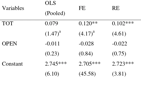
group of countries with lower wage dispersion (see Table 2). On the other hand, for the

group of countries with higher wage dispersion (see Table 1) although the estimated

coefficient of the TOT in the pcgdp is positive it is not statistically significant in all the

three panel data models. However, one thing should be noted that the signs of the

estimated parameters for the coefficient of TOT are remarkably consistent and intuitively

[Insert Table 1 is about here]

Table 1: Panel data analysis with countries having higher wage dispersions

Variables OLS

(Pooled) FE RE

TOT 0.019

(0.60)a

0.007 (0.23)

0.013 (0.46) OPEN 0.071**

(2.12)

0.091* (2.42)

0.082** (2.10) Constant 2.866***

(11.28)

2.877*** (32.87)

2.872*** (8.21)

a

t-value (corresponding to robust standard error) in parentheses.

*** Significant at 1% level. ** Significant at 5% level. * Significant at 10% level.

[Insert Table 2 is about here]

Table 2: Panel data analysis with countries having lower wage dispersions

Variables OLS

(Pooled) FE RE

TOT 0.079

(1.47)a

0.120** (4.17)a

0.102*** (4.61) OPEN -0.011

(0.23)

-0.028 (0.84)

-0.022 (0.75) Constant 2.745***

(6.10)

2.705*** (45.58)

2.723*** (3.81)

a

t-value (corresponding to robust standard error) in parentheses.

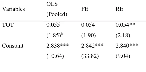
To check the robustness of the above findings, we have also considered this analysis

without considering the control variable OPEN. Results relating to higher wage

dispersion countries are reported in Table 3 whereas the estimates corresponding to lower

wage dispersion countries are reported in Table 4. These results also support our

analytical finding that countries with higher wage dispersion are relatively less affected

by TOT fluctuations of recent years compared to those countries with lower wage

dispersion.

[Insert Table 3 is about here]

Table 3: Panel data analysis with countries having higher wage dispersions

Variables OLS

(Pooled) FE RE

TOT 0.055

(1.85)a

0.054 (1.90)

0.054** (2.18) Constant 2.838***

(10.64)

2.842*** (33.82)

2.840*** (9.04)

a

t-value (corresponding to robust standard error) in parentheses.

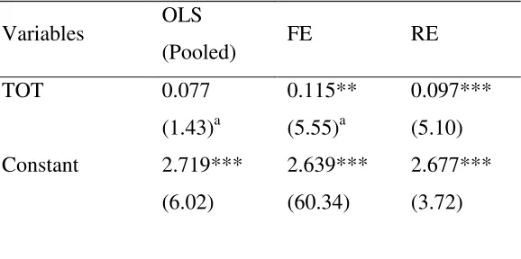
[Insert Table 4 is about here]

Table 4: Panel data analysis with countries having lower wage dispersions

Variables OLS

(Pooled) FE RE

TOT 0.077

(1.43)a

0.115** (5.55)a

0.097*** (5.10) Constant 2.719***

(6.02)

2.639*** (60.34)

2.677*** (3.72)

a

t-value (corresponding to robust standard error) in parentheses.

*** Significant at 1% level. ** Significant at 5% level. * Significant at 10% level.

To decide between the FE and RE for the appropriate model particular to our dataset we

have conducted well-known Hausman test where the null hypothesis considers that the

preferred model is the RE model and have found that we fail to reject the null hypothesis.

Thereafter, we have proceeded by conducting the Lagrange Multiplier (LM) test for the

panel effect with the null hypothesis that the variance across countries is zero. The result

indicates that we fail to accept the null hypothesis which in turn substantiates our

empirical analysis with panel data instead of considering separate OLS regression for

each country. Moreover, in view of the short time span and assumed parameter

homogeneity, following Baltagi et al. (2009), we can conclude that the panel results

should be more reliable vis-a-vis pooled OLS results (given in the first column in each of

This result suggests that, on average, a 1% increase in TOT across time and between

countries with lower wage dispersion caused about 0.1% overall increase in the pcgdp

whereas countries with higher wage dispersion had experienced either no (see Table 1)

or lower (almost half) impact (0.05%, see Table 3) of TOT changes on the pcgdp. Hence,

our findings are as follows: the effect of TOT changes on pcgdp growth had been

typically small in absolute terms but consistently significant relative only to the

developing countries with lower wage dispersion. These results provide systematic

econometric evidence to support the hypothesis that the TOT changes had significant

impact on economic growth in the countries with lower wage dispersion but negligible

impact on growth in higher wage dispersion countries during the period, 2000-2012.

4. Concluding remarks and policy recommendations

Some recent empirical studies have found that developing countries are more prone to

external terms-of-trade shocks compared to developed nations. Policies like switching

from fixed to flexible exchange rate regime and diversification of the export basket have

been advocated in general to minimize the negative effects resulting from such

international disturbances. However, possibly no attempt has been made to identify the

inherent shock-absorbing mechanism in the developing countries which arises out of their

typical institutional characteristics. In this study, we have demonstrated how the

existence of labor market imperfection can lessen the gravity of detrimental TOT shocks

on social welfare. Moreover, by examining cross-country data we substantiate our

findings that countries with relatively higher intersectoral wage differential have

period 2000-2012 relative to the other set of countries with smaller wage dispersion. We

are of the opinion that the developing countries should not go for labor market reforms

because these would impair the effectiveness of their internal shock-absorbing capacity

against adverse international price movements.

References:

Baltagi, B.H., Demetriades, P.O. and Law, S.H. (2009): ‘Financial development and openness: Evidence from panel data’, Journal of Development Economics 89(2), 285-296.

Baxter, M. and Kouparitsas, M. A. (2006): ‘What can account for fluctuations in the terms of trade?’, International Finance 9(1), 63-86.

Broda, C. (2004): ‘Terms of trade and exchange rate regimes in developing countries’,

Journal of International Economics 63(1), 31-58.

Broda, C. and Tille, C. (2003): ‘Coping with terms-of-trade shocks in developing countries’, Current Issues in Economics and Finance 9(11), Federal Reserve Bank of New York.

Chaudhuri, S. and Mukhopadhyay, U. (2014): “Foreign Direct Investment in Developing Countries: A Theoretical Evaluation”, Springer, New Delhi, India.

Chaudhuri, S. and Mukhopadhyay, U. (2009): “Revisiting the Informal Sector: A General Equilibrium Analysis”, Springer, New York.

Edwards, S. and Levy-Yeyati, E. (2003): ‘Flexible exchange rates as shock absorbers’,

Haddad, M., Lim. J., Munro, L., Saborowski and Shepherd, B. (2011): ‘Volatility, export diversification, and policy’. In M. Haddad and B. Shepherd Eds.), Managing Openness:

Trade and Outward-oriented Growth after the Crisis, World Bank Publications, Chapter

11.

Hoffmann, M. (2007): ‘Fixed versus flexible exchange rates: evidence from developing countries’, Economica 74(295), 425-449.

Mendoza, E. G. (1995): ‘The terms of trade, the real exchange rate, and economic fluctuations’, International Economic Review 36(1), 101-37.

Kose, M.A. (2002): ‘Explaining business cycles in small open economies: How much do world prices matter?’ Journal of International Economics 56(2), 299-327.

Tornell, A. and Velasco, A. (2000): ‘Fixed versus flexible exchange rates: which provides more fiscal discipline?’ Journal of Monetary Economics 45(2), 399-436.

World Bank: World Development Indicators of the World Development Report(s). Washington, DC.