Munich Personal RePEc Archive
Are Behaviours in the "11-20" Game
Well Explained by the level-k Model?
Choo, Lawrence C.Y and Kaplan, Todd R.
University of Exeter, University of Haifa
9 February 2014
Are Behaviours in the “11-20” Game Well Explained by the level-k
Model?
∗Lawrence C.Y Choo† Todd R. Kaplan‡
This Version: February 2014
Abstract
We investigate whether behaviours in Arad and Rubinstein (2012) “11-20” game are well
explained by the level-k model. We replicate their game in our Baseline experiment and provided
two other variations that retain the same mixed-strategy equilibrium but result in different
predicted level-k behaviours. Our hypothesis test is motivated by the logic that if the Baseline
and variation games capture level-k reasoning behaviours, we should find consistent proportion
of level-k types in all games. We considered two types of level-k models where players were
assumed to best respond stochastically and found that the level-k models were able to explain
the data significantly better than the equilibrium driven alternatives. In addition, the
level-k models were also able to demonstrate consistent proportions of level-level-k types between the
differentiated games. Our findings provide support for Arad and Rubinstein (2012) assertion
that behaviours in the “11-20” game can be attributed to the level-k models.
Keywords: level-k, Cognitive Hierarchy, Quantal Response Equilibrium, 11-20 Game
JEL-Classification: C73, C91
⇤
We are grateful to the suggestions and comments of participants at the 4th Annual Xiamen University Interna-tional Workshop on Experimental Finance.
†University of Exeter. Corresponding Author. Email:
1
Introduction
Deviations from equilibrium predictions are often documented in the literature of economic and
game theory experiments. The challenge in this field is the provision of better explanatory tools.
One explanation posits that players often avoid the circular concepts embedded in equilibrium
outcomes, and instead make use of rule-of-thumb behaviours (Crawford et al.,2013). Furthermore,
this explanation suggests that such behaviours are associated with the finite steps of iterative
reasoning those players are able to employ. The level-k model (Nagel, 1995; Stahl and Wilson,
1994, 1995; Costa-Gomes et al., 2001) and the closely related Cognitive Hierarchy (CH) Model
(Camerer et al.,2004) are leading candidates in this field.
The general level-k model (we will use the term “level-k” to include the CH model and make
the distinction where necessary) partitions the population of players into specificLktypes, wherek
denotes the steps of iterative reasoning those players are able to employ. The model anchors upon a
non-strategicL0 type, who is assumed to follow some behavioural specification. Such specification
is analogous to players’ instinctive reaction in the game and is often taken to be the uniform
randomisation over all strategies.1 Higher L
k types (k > 0), hold beliefs about the proportion of
lower types in the population and best respond to these beliefs via iterative though-experiments.
For example, if each higher type believes that everyone else is exactly one type below, the model
predicts that aL1 type will choose the strategy that is a best response to theL0 type’s behavioural
specification, a L2 type to a L1 type’s strategy, a L3 type to a L2 type’s strategy, and so forth.
Higher types are thus strategic in the same tradition of “rationalizable strategies” (Bernheim,1984;
Pearce,1984).
The level-k model is simple and intuitive, however applications to wider economic settings first
requires some prior on the plausible proportions of types and the beliefs of each higher types. This
has led to a growing body of literature that examined the level-k model in laboratory experiments
and in the field (seeBosch-Dom`enech et al.,2002;Brown et al.,2013;Ostling et al.¨ ,2011). However,
1
Whether the uniform randomisation is the appropriate specification of the L0 type’s behavioural is by itself a
debate. Such specification is attractive since it iscontext freeand easily portable to a variety of games. However, in some games, this also meant that theL0 type player assigns equal weights to strategies that are payoffdominant and
such investigations naturally leads to concerns as to whether (a) The L0 types’s specification is
salient amongst the pool of subjects, (b) The beliefs of higher types are correctly specified and (c)
Best responding behaviours driven by iterative thought-experiments are natural. If this is not the
case, then any estimated or derived proportions of Lk types may likely be misleading.
To address these concerns,Arad and Rubinstein(2012) - henceforth known as AR - proposed the
“11-20” game to study the level-k model. The game involves two players simultaneously choosing
an integer between 20.00 to 11.00, which corresponds to the equivalent amount of payoffs that they
would each receive with certainty. In addition, a player receives a bonus payoff of 20.00, if his chosen integer is 1.00 less than the other player’s. The game has no pure-strategy equilibrium, but
a mixed-strategy equilibrium that assigns positive probabilities to the strategies 20.00 to 15.00.
In AR’s experiments, subjects’ behaviours were significantly different from the mixed-strategy
equilibrium and they proposed the level-k model to capture such deviations. Four assumptions
were made in their analysis (1) Players seek to maximise their individual payoffs, (2) The L0 type
player will always choose 20.00, (3) HigherLk types believes that all other players are exactly one
type below and perfectly best respond to such beliefs, and (4) There exist a highest possible type
LK¯ = 9. The authors highlighted the saliency of their L0 type’s behavioural specification in the
game as it corresponds to the highest payoffthat a player could receive without consideration for
the behaviours of other players. Given these assumptions, the L1 type players will best respond
with 19.00, theL2 types with 18.00, the L3 types with 17.00 and so forth.2 Therefore, the relative
proportions ofLk types could be directly inferred from the observed aggregated strategies in game.
TypesL1,L2andL3 were most frequently found in the proportions 0.12, 0.30 and 0.32 respectively.
Subsequent adaptions of the “11-20” game were employed byLindner and Sutter (2013) to study
decision making under time pressure and Alaoui and Penta (2013) to study endogenous iterative
reasoning.
Do behaviours in the “11-20” game necessarily correspond to those predicted by the level-k
model? Might the game be too simple to capture the level-k reasoning behaviours? The premise of
the level-k model is that subjects who doksteps of iterative thought-experiments to not expect any
2
Without the boundLK¯ = 9 on the distribution of types, AR’s level-k reasoning process inducescycles, such that
other players to do k+ 1 steps, otherwise they would respond with k+ 2 steps. This justification
is usually found in the psychological evidence of overconfidence in one’s abilities (seeCamerer and
Lovallo, 1999; DellaVigna, 2009). Therefore, one should expect each additional step of iterative
thought-experiments to be less obvious or more cognitively demanding. However, the nature of
the “11-20” game meant that subjects who do one step of iterative thought-experiment could
easily extend it to two steps or more without significantly more cognitive effort.3 Given these,
shouldn’t one expect higher types e.g., L4, L5, L6, to be more frequently observed in the
“11-20” game? Alternatively, could subjects’ behaviour in the game be better explained by some
statistical distortion of the mixed-strategy equilibrium such as in the Quantal Response Equilibrium
(McKelvey and Palfrey, 1995, 1996, 1998)? Ultimately with experimental data, there could be
multiple competing explanations. The question here is whether the level-k model is the dominant
explanation as AR had proposed. This is an open questions left by AR’s discussions and the
challenge is to put forth a suitable experimental design to investigate.4
Denoting the “11-20” game as the Baseline game, we propose the following two simple
ex-tensions, the Medium and Extreme games. In the Medium game, players choose from following
strategies 20.00, 19.50, 19.00,..., 11.00, which they are certain to receive in equivalent payoffs. The bonus of 20.00 is only awarded if the player’s strategy is 0.50 or 1.00 less than the other player.
In the Extreme game, players choose from the strategies 20.00, 19.75, 19.50, 19.25, 19.00,..., 11.00,
which they are again certain to receive in equivalent payoffs. However, the bonus of 20.0 is now
only awarded if the player’s strategy is 0.25, 0.50, 0.75or 1.00 less than the other player. All games
- Baseline, Medium and Extreme - share the same decisional structure and problem as the “11-20”
game. In addition, the games also have equivalent mixed-strategy equilibrium distributions (see
3
One of the most frequently discussed game in the level-k literature isNagel(1995) guessing game. Here a group (n 2) of players simultaneously choose a number from 0 to 100. A fixed prized is awarded to that player whose number is closest to 2/3 of the average. If aL0 type player is assumed to uniformly randomise across all numbers, a
shouldL1 best respond to the uniform randomisation. AL2 should best respond to the best response of a uniform
randomisation. AL3should best respond to the best response of a best response to a uniform randomisation, and so
forth. Owning to the game’s design, the best responding task becomes more challenging or computationally difficult, as the step of iterative thought-experiments increases.
4
In their paper, AR also considered two other extension of the “11-20” game, the costless iteration and cycle
Table1). For example, the strategies {20.00} in the Baseline game, {20.00,19.50}in the Medium
game and {20.00,19.75,19.50,19.25} in the Extreme game are all predicted to be chosen with 5%
probability. Similarly, the strategies{19.00},{19.00,18.50} and{19.00,18.75,18.50,18.25}, in the
Baseline, Medium and Extreme games respectively, are predicted by the mixed-strategy equilibrium
to be chosen with 10% probability.
However, when approached by the level-k model, the strategies in the respective games are
predicted to be chosen by noticeably different Lk types. To see why this might be so, consider the
AR’s level-k analytical approach. In all games, theL0 type is again assumed to choose the 20.00.5
Higher types are assumed to believe that everyone else is one type below and the distribution of
types are bounded at LK¯ = 9,16,36, the Baseline, Medium and Extreme games respectively. The
L1 type will best respond with 19.00, 19.50 and 19.75, in the Baseline, Medium and Extreme games
respectively. TheL2 type with 18.00, 19.00 and 19.50, the L3 type with 17.00, 18.50, and 19.25,
and so forth in the respective games. As such, if the level-k model is the dominant explanation to
players’ behaviours in the respective games, we should expect the inferred or estimated proportions
of Lk types to be consistent between the differentiated games if players were randomly recruited
from the same population. This presents us with a simple hypothesis test.
Our experiments involved four classroom sessions, conducted over two cohort of students.
Stu-dents in the first cohort were recruited into the Baseline and Medium games, whilst those in the
second cohort were recruited in the Medium and Extreme games. Our hypothesis test hence makes
comparisons between the level-k model’s inferred or estimated proportions of types in session of
the same cohort.
In our first set of test, we adopted AR’s analytical approach, where the proportions of Lk
types were directly inferred from the aggregated strategies of the respective treatments. In each
comparisons, the proportions of types were found to be significantly different. Whilst this might not exclude the possibility that subjects’ behaviour could be explained by a more generalised form
of level-k model, it clearly highlights the limitations of AR’s analytical approach.
In our second set of test, we relaxed some of the assumptions behind AR’s analytical approach,
5
In each game, theL0type should always choose the strategy 20.00, since it still corresponds to the highest payoff
allowing for higher types to best respond stochastically. This allows us to consider two types of
level-k models, the SK model (higher types believe that everyone else is one type below) and the CH
model (higher type believes that everyone else is a mixture of lower types). We fitted the sessions’
data with both models to estimate the proportions ofLk types. In addition, we also examined the
statistical fit of the Quantal Response Equilibrium (QRE). ThroughVuong (1989) likelihood ratio
test, the SK and CH models were found to have fitted the data significantly better than the QRE
and the mixed-strategy equilibrium, but as well as each other. Returning to our main hypothesis
test, the estimated proportions of types in the CH model were not found to be significantly different. Similarly, the estimated types in the SK model were not found to be significantly in the second
cohort and to a lesser extend, the first cohort. These results provide evidence that the level-k
models may have been the dominant explanation to subjects’ behaviours in our experimental data
and quite possibility the “11-20” game. In other words, our results provide some robustness support
to AR’s assertion on the “11-20” game’s suitability on studying the level-k model.
The rest of this paper is organised as followed: Section 2 details our experimental procedures,
Section3provides an overview of the data and investigate AR’s level-k analytical approach, Section
4 formally introduces the SK and CH models, Sections 5 reports the estimated results of the SK,
CH and QRE models and finally, Section6 concludes.
2
Experiment Procedure
Four classroom experimental sessions were conducted at the University of Exeter, over two cohorts
of Intermediate Microeconomics students. The subjects were mostly economics majors and with no
formal training in game theory. We denote each session by the game which the subjects were enrolled
into - Baseline(B), Medium(M) and Extreme(E), followed by the cohort which they were recruited
from. For example, session B(2012) refers to the Baseline game conducted with subjects from
cohort 2012. All sessions were conducted during the first lecture class of the course (approximately
250-300 students in each class) and subjects were informed that their participation was voluntary.6
In each cohort, the layout of the lecture class had consisted of three separated seated columns.
6
With cohort 2012 and 2013, subjects in the centre seated column received the instructions for
sessions B(2012) and M(2013) respectively. Subjects in the two other side columns received
in-structions for sessions M(2012) and E(2013) respectively. The inin-structions were as followed:
Baseline (B) Game: You and another player will simultaneously request an amount of payoff
from the set {2000, 1900, 1800, 1700, ..., 1100} denoted in ECU. Each player will receive his
chosen amount. In addition, a player will receive a bonus of 2000 if his request amount is 100 ECU
less than the other player.
Medium (M) Game: You and another player will simultaneously request an amount of payoff
from the set {2000, 1950, 1900, 1850, ..., 1100} denoted in ECU. Each player will receive his
chosen amount. In addition, a player will receive a bonus of 2000 if his request amount is (a) 50
ECU or (b) 100 ECU less than the other player.
Extreme (E) Game: You and another player will simultaneously request an amount of payoff
from the set {2000, 1975, 1950, 1925, 1900, ..., 1100} denoted in ECU. Each player will receive
his chosen amount. In addition, a player will receive a bonus of 2000 if his request amount is (a)
25 ECU, (b) 50 ECU, (c) 75 ECU or (d) 100 ECU less than the other player.
Subjects had to circle their choice on a table consisting of all the relevant request amounts. In
addition, subjects were to include their contact details and a brief feedback of their behaviour. The
sessions were completed within 15 minutes and the instruction sheets were thereafter collect by the
experimenters. In each cohort, ten pairs of subjects were randomly selected for cash payment (they
were privately contacted via email) at the exchange rate of 100 ECU to 1 British pound. A total
of 130, 140, 114 and 94 subjects participated in sessions B(2012), M(2012), M(2013) and E(2013),
respectively.
We choose to split the sessions by the seated columns for ease of instructions distribution
and to avoid any confusion created by subjects seeing the other instructions. However, the same
experimental procedure induce concerns that there might be some natural differences in behaviours
due to the seated positions of subjects.7
7
To address such concerns, the respective sessions were immediately followed up by the Guessing
Game (Nagel, 1995).8 Here each player chooses a number between 0 to 100 and a fixed prized
is awarded to the player whose chosen number is closest to 2/3 of the average. Subjects in each
cohort competed against each other for a fixed prize of 50 British pound, were informed that the
Guessing Game was a different experiment from the previous sessions and that their participation
was voluntary. The Guessing Game instructions sheets were distributed and collected within 20
minutes. A total of 274 and 206 subjects participated in the Guessing Game for cohorts 2012 and
2013 respectively.
To control for our concerns in the sessions’ data, we had firstly excluded all observations where
subjects had not participated in the Guessing Game. Thereafter, in each cohort, we employed
the k-mean clustering algorithm to identify equal session sample sizes, such that the cumulative
distribution of Guessing Game numbers in each session sample was not significantly different from each other. 9 This resulted in 117 and 91 observations in each session of cohort 2012 and 2013
respectively.
3
Experimental Results
The sessions’ results are summarised in Table1. The first and second columns refer to the strategies
and mixed-strategy equilibrium predictions respectively, whilst the third column to sixth columns
refer to the observed frequency of strategies in the respective session. As an empirical warm-up, we
first investigated if subjects’ behaviours were consistent with the mixed-strategy equilibrium. Here,
Fisher’s exact test finds all sessions’ data to be significantly different (two-sided Fisher ⇢< 0.001
for all comparisons).10
Result 1: Behaviours in B(2012), M(2012), M(2013) and E(2013) were found to be significantly
8
We employed the Guessing Game since it was one the most frequently studied game in the level-k literature.
9
We verified these results with the Kolmogorov-Smirnov test which reports a p-value of 0.242 (0.453) in cohort 2012 (2013).
10
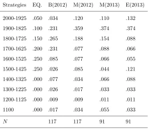
Table 1: Summary of Observed Strategy Frequencies and Mixed-Strategy Equilibrium
Strategies EQ. B(2012) M(2012) M(2013) E(2013)
2000-1925 .050 .034 .120 .110 .132
1900-1825 .100 .231 .359 .374 .374
1800-1725 .150 .265 .188 .154 .088
1700-1625 .200 .231 .077 .088 .066
1600-1525 .250 .085 .077 .066 .055
1500-1425 .250 .026 .085 .044 .121
1400-1325 .000 .077 .034 .066 .088
1300-1225 .000 .026 .017 .033 .033
1200-1125 .000 .009 .009 .011 .011
1100 .000 .017 .034 .055 .033
N 117 117 91 91
different from the mixed-strategy equilibrium.
A prominent difference pertains to the strategies 1600-1425, which although predicted by the
mixed-strategy equilibrium to be chosen by 50% of the subjects in each session, were only observed
to be chosen by no more than 18% in any session. Comparing between sessions of the same game,
the B(2012) session data was not found to be significantly different from AR’s results (two-sided Fisher ⇢ = 0.323).11 Similarly, the M(2012) and M(2013) sessions’ data were not found to be
significantly different (two-sided Fisher⇢= 0.483).
Result 2: Behaviours in the B(2012) were not found to be significantly different to those inArad
and Rubinstein(2012) experiments and those in M(2012) were not found to be significantly different
in M(2013).
These results suggest that there might be some coherent structure in the behaviour of subjects.
11
This finding was also shared in replications of the “11-20” game byLindner and Sutter(2013) andGoeree et al.
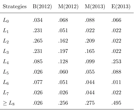
Table 2: Inferred proportion of Lk types by the Arad and Rubinstein (2012) level-k Analytical
Approach
Strategies B(2012) M(2012) M(2013) E(2013)
L0 .034 .068 .088 .066
L1 .231 .051 .022 .022
L2 .265 .162 .209 .022
L3 .231 .197 .165 .022
L4 .085 .128 .099 .253
L5 .026 .060 .055 .088
L6 .077 .051 .044 .011
L7 .026 .026 .044 .022
≥L8 .026 .256 .275 .495
The question here is whether this structure pertains to the level-k model as suggested by AR. To
investigate, we first adopted AR’s analytical approach, where the proportions of Lk types were
directly inferred from the aggregated strategies. This approach assumes that (1) Players seek to
maximise their individual payoffs, (2) The L0 type will always choose 2000, (3) Higher Lk types believe everyone else to be one type below and always perfectly best respond to such beliefs and
(4) The distribution of types are bounded atLK¯ = 9,16,36 in the Baseline, Medium and Extreme
games respectively. Given these assumptions, we report on Table2 the inferred proportions of Lk
types (truncated at theL8 type) in the respective sessions.
To test our hypothesis that the level-k model was the dominant explanation to subjects’
be-haviours, comparisons were made between sessions of the same cohort. In cohort 2012, the inferred
proportions of Lk types were found to be significantly different (two-sided Fisher ⇢ < 0.001). In
session B(2012), 73% of subjects were classified as typesL1−L3 whilst the same classification only
pertains to 41% of subjects in M(2012).
typesL1−L3, only 7% of subjects in session E(2013) fall under the same classification. Furthermore,
a quarter of all subjects in session E(2013) had chosen the amount 1900, which corresponds to the
L4 type.
Result 3: Arad and Rubinstein (2012) level-k analytical approach leads to significantly different
inferred proportions of Lk types between sessions of the same cohort.
This result could either imply that behaviours in the respective sessions (and consequently the
“11-20” game) were inconsistent with the level-k model or that the behaviours were consistent with
the level-k model but AR’s level-k analytical approach was limited in its extend to explain such
behaviour. To avoid“throwing the baby out with the bathwater”we decided to go with latter point
and relax some of AR’s assumptions in the next section.12
4
Level-K Models with Stochastic Best Response
In this section, we relax AR’s assumptions, allowing for higher types to best respond stochastically,
with the introduction of a common noise ≥ 0 parameter. This allows us to consider two types
of level-k models, the stochastic level-k (SK) model and the Cognitive Hierarchy (CH) model.
Such approach naturally leads to comparisons with the Quantal Response Equilibrium (QRE), the
rational expectation “statistical refinement” of the mixed-strategy equilibrium. To provision for a
common platform of comparisons, we will assume that the individual probability choice function
takes the logistic functional form (McFadden,1976). In the following sub-section, we will formally
introduce the SK and CH models. Discussion of the QRE are omitted since it is well known in the
literature.
12
One may disagree with our hypothesis test. More specifically, why should the level-k model imply consistent proportions ofLktypes between sessions of the same cohort? In our view, this alternative is merited if the respective
sessions involved games that were intrinsically different. However, in the setting of our experiment, this alternative propounds that small modifications to the game results in its own unique proportions of Lk types. Whilst such
4.1 The SK and CH models
The SK and CH models consider a hierarchical of Lk types but differ on their assumed beliefs
for each higher types. In applications to our Baseline, Medium and Extreme games, both models
involve i = 1,2 players, each simultaneously choosing a strategy ai ∈ A. Denote ⇡i(ai, a−i) > 0
as the payoff to player i for choosing strategy ai if the other player chooses a−i. Both models anchor upon a non-strategicL0 type who is assumed to always choose the strategy 2000. For any
higher Lk type player i, let bki(g) ∈ [0,1] denote the proportion of Lg type players he believes to
exist in the population. We assume that bk
i(g) = 0 for all g ≥k, implying that players ignore the
possibility that other players might be the same or higher types than himself.13 The SK model
assumes that each higherLk type believes everyone else to be exactly one type below, resulting in
beliefsbk
i(g) = 1 if and only if g=k−1 or otherwise 0.
On the other hand, the CH model assumes that each higher Lk type believes everyone else to
be a mixture of lower types, distributed accordingly to a normalised Poisson distribution. More
specifically, for any population of players, letf(k)∈[0,1] denote the true proportions ofLk types.
The CH model therefore assumes that f(0), f(1), ..., f(k),... follows a Poisson distribution with
the mean and variance ⌧, where f(k) = ⌧kexp(−⌧)/k!. The CH model also makes a simplifying
assumption that each higher type knows the true relative proportions of lower types, resulting in
beliefs
bki(g) = Pk−f(1g|⌧) h=0f(h|⌧)
∀k >0, g < k
If the true proportions of types are clustered around the lower types, then an interesting consequence
of the CH model relative to the SK model, is that the beliefs of higher types in the former model
become more precise ask increases, whereas the beliefs in latter becomes less precise.
Let pk(a
i)≥0 denote the probability of a higher type playerichoosing strategy ai ∈A
pk(ai) =
exp( ⇡i(ai,·)) P
a0i∈Aexp( ⇡i(a
0
i,·))
∀k >0
where⇡i(ai,·) =Pa i∈A⇡i(ai, a−i){ Pk−1
g=0bki(g)·pg(a−i)}denotes the expected payofffor a higher
13
Solving a model wherebk
i(g)6= 0 forg=kmight also be more complex and involve finding a fixed point at each
Lktype playeriwith choosing strategyai.14,15As → ∞, each higher type places more weights to the strategy that accords to him the highest payoff. Likewise as →0, each higher type uniformly randomises across all strategies.16
With data, the SK and CH models will be fitted through econometric methods. The
econo-metric results make two predictions, the common noise and the proportions ofLk types. We are
primarily interested in the latter predictions. The estimation of the SK model first requires some
prior arbitrary specification of LK¯ = 2,3,4, ..., the highest type one believes to exist in the data.
Thereafter, the proportions of types, L0 through toLK¯, and the noise parameter are estimated
from the data (this results in ¯K+ 1 free parameters). Since the SK model does not impose any
parametric restrictions on the distribution of types, it presents one with certain amount of
flexibil-ity in increasing the statistic fit by considering differentLK¯. Estimation of the CH model usually
involves setting an arbitrary highLK¯. Thereafter, the parameters ⌧ and are estimated from the
data given the restriction that 1−PKk¯=0f(k) < ✏. One should note that given the parametric assumptions on the distribution of types, the CH model is slightly more restrictive than the SK
model. However, is such restriction tantamount to a significantly worst fit?17
14
One could also model the choice probability function with the normalised power function
pk(ai) =
(πi(ai,·))
λ
P a0
i2A(
πi(a0i,·))
λ 8k >0
as inOstling et al.¨ (2011), and the results will most probability be identical. We decided upon theLogisticfunctional form for natural comparisons against the QRE model.
15
An alternative specification is to assume that the higher Lk types will uniformly randomise with probability
εk2[0,1] or choose the action which accords the highest expected payoffwith probability (1 ε) as inCosta-Gomes
et al.(2001). This alternative may not be immediately applicable to the CH model. Since our objective is to restrict any behavioural differences between the SK and CH models to assumptions on higher types’ beliefs, we choose not to adapt this alternative specification.
16
AR’s level-k analytical approach is a special case of the SK model whereλis fixed at infinity.
17
In applications to a series of Guessing Game results,Camerer et al.(2004) adaption of the CH model estimated
τ ⇡ 1.61 (types L1 and L2 most frequent). They found that the CH model had fitted the data as well as the
conventional level-k model (each higherLk believes everyone else to be one type below). Given that the prescribed
behaviour of players in the two models only differ from typeL2 onwards, we do not find their results surprising since
most level-k study on the guessing game also found typesL1 andL2to be most frequent. Results in this experiment
5
Econometric Results
The estimates from the SK and CH models and the QRE were derived through maximum likelihood
estimation (see Appendix for discussion of MLE procedures in the level-k models). To avoid
over-fitting the SK model, we first estimated B(2012) with highest type LK¯ = 3,4,5,6,7,8,9. At the
1% significance level, the likelihood ratio test prefers the estimates whereLK¯ = 6. The remaining
sessions were hence estimated with LK¯ = 6. The CH model was estimated by setting LK¯ = 16.
However, for the purposes of this presentation, we will only report the estimated proportions of
types for 0 ≤ k ≤ 6. To do so, we normalised the proportions of types in the same approach
demonstrated byKawagoe and Takizawa (2012).18
We report on Tables3and 4the estimation results for sessions in cohort 2012 and 2013
respec-tively. We also included the mixed-strategy equilibrium for comparisons . Each table comprises
of three panels. The top panel depicts the observed and the predicted frequency of strategies by
the mixed-strategy equilibrium, QRE, SK and CH estimates. The middle panel reports the test
statistics of Vuong (1989) likelihood ratio test - to be discussed in sub-section 5.1. The bottom
panel reports the proportions of Lk types as estimated by the SK and CH models. We also fitted
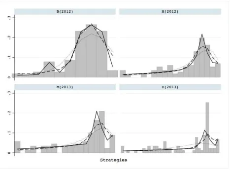
on Figure 1, the predicted frequency of strategies by the QRE (dotted lines), SK (solid lines) and
CH (dashlines) estimates.
In the following discussions, we will first focus on the statistical fit of each model. If the level-k
models (SK and CH) were found to have explained the data significantly better than the equilibrium
driven alternatives (QRE and mixed-strategy equilibrium), we will return to our main hypothesis
test, where comparisons of the level-k models’ estimates will be made between sessions of the same
cohort. This serves as a robustness check on theinformativeness of the level-k estimates, whether
they were mere statistical phenomenons or better representation of subjects’ behaviours.19
18
The CH model’s estimated proportions ofLktypes were derived byf(k)/P
6
h=0f(h), wheref(k) =τ
k
exp( τ)/k!.
19
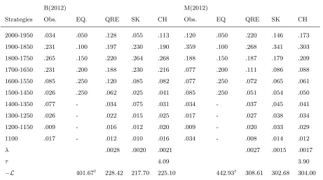
Table 3: Cohort 2012: Observed and Predicted Frequency of Strategies by the Mixed-Strategy
Equilibrium, QRE, SK and CH
B(2012) M(2012)
Strategies Obs. EQ. QRE SK CH Obs. EQ QRE SK CH 2000-1950 .034 .050 .128 .055 .113 .120 .050 .220 .146 .173 1900-1850 .231 .100 .197 .230 .190 .359 .100 .268 .341 .303 1800-1750 .265 .150 .220 .264 .268 .188 .150 .187 .179 .209 1700-1650 .231 .200 .188 .230 .216 .077 .200 .111 .086 .088 1600-1550 .085 .250 .120 .085 .082 .077 .250 .072 .065 .061 1500-1450 .026 .250 .062 .025 .041 .085 .250 .051 .054 .050 1400-1350 .077 - .034 .075 .031 .034 - .037 ,045 .041 1300-1250 .026 - .022 .015 .025 .017 - .027 .038 .034 1200-1150 .009 - .016 .012 .020 .009 - .020 .033 .029 1100 .017 - .012 .010 .016 .034 - .008 .014 .012
λ .0028 .0020 .0021 .0027 .0015 .0017
τ 4.09 3.90
L 401.67† 228.42 217.70 225.10 442.93† 308.61 302.68 304.00 †: Log-likelihood derived by assigning the mass of 0.000001 to non-equilibrium strategies
Vuong test EQ QRE CH EQ QRE CH
SK 4.83a
2.80a
2.11b
SK 4.36a
1.67b
0.60 CH 4.81a
1.68b
CH 4.38a
2.27b
QRE 4.73a
QRE 4.30a a
:ρ<0.1;b
:ρ<0.05 andc
:ρ<0.01 (one-sided test)
Model Session L0 L1 L2 L3 L4 L5 L6
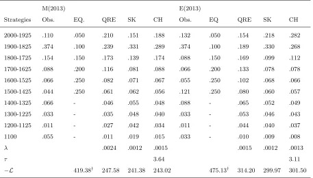
Table 4: Cohort 2013: Observed and Predicted Frequency of Strategies by the Mixed-Strategy
Equilibrium, QRE, SK and CH
M(2013) E(2013)
Strategies Obs. EQ. QRE SK CH Obs. EQ QRE SK CH 2000-1925 .110 .050 .210 .151 .188 .132 .050 .154 .218 .282 1900-1825 .374 .100 .239 .331 .289 .374 .100 .189 .330 .268 1800-1725 .154 .150 .173 .139 .174 .088 .150 .169 .099 .112 1700-1625 .088 .200 .116 .081 .088 .066 .200 .133 .078 .078 1600-1525 .066 .250 .082 .071 .067 .055 .250 .102 .068 .066 1500-1425 .044 .250 .061 .062 .056 .121 .250 .080 .060 .057 1400-1325 .066 - .046 .055 .048 .088 - .065 .052 .049 1300-1225 .033 - .035 .048 .040 .033 - .053 .046 .043 1200-1125 .011 - .027 .042 .034 .011 - .044 .040 .037 1100 .055 - .011 .019 .015 .033 - .010 .009 .008
λ .0024 .0012 .0015 .0015 .0012 .0013
τ 3.64 3.11
L 419.38† 247.58 241.38 243.02 475.13† 314.20 299.97 301.50 †: Log-likelihood derived by assigning the mass of 0.000001 to non-equilibrium strategies
Vuong test EQ QRE CH EQ QRE CH
SK 5.01a
1.89b
0.68 SK 5.24a
3.01a
0.81 CH 5.07a
2.68a
CH 5.22a
2.73a
QRE 5.04a
QRE 4.76a a
:ρ<0.1;b
:ρ<0.05 andc
:ρ<0.01 (one-sided test)
Model Session L0 L1 L2 L3 L4 L5 L6
Figure 1: Observed and Predicted Frequency of Strategies - SK (Solid Lines); CH (Dash Lines);
5.1 Comparing Statistical Fit
Since the models are non-nested, our comparison approach will employVuong(1989) likelihood ratio
test. The test assumes that there exist a true model, and with pairwise comparisons, evaluates
which of two models is “closer” to the true model. The Null hypothesis is for both models to
be equally close and the test provisions for two one-sided Alternative hypotheses, that one of the
two models is significantly closer.20,21 The test statistic is assumed to follow a standard normal
distribution.
For the ease of interpretation, the test statistics are presented in the following manner: With
pairwise comparisons, the model with more (less) favourable log-likelihood value will be positioned
in the row (column) - this ensures that the test statistics must be positive. This allows us to
conduct a simple one-sided test to evaluate if the row model fits the data significantly better than
the column model. In the following, we shall use the terms “out-performed” and “tied” to denote
the outcome of the likelihood ratio test between two models. For example, A is said to have
out-performed B, if the likelihood ratio test finds A significantly closer to the true model. Similarly, A
is said to have tied with B, if one is unable to reject the null hypothesis.
In all comparisons, the QRE, SK and CH were found to have out-performed the mixed-strategy
equilibrium. This should not be surprising since the former three were econometrically fitted onto
the data. The following discussions will hence focus on the former three.
B(2012): The SK and CH were found to have out-performed the QRE, but the SK was
also found to have out-performed the CH. From top left box of Figure 1, these findings become
more apparent. The SK model tracks the strategies 2000-1400 much better than the other two
models. However, this could also be driven by the fact that such strategies largely correspond to
the behaviour profiles of typesL0−L6, which were by construct free parameters in the SK model.
20
The Vuong (1989) test suffers from some logical issues if two fundamentally different models i.e. Rational expectation and Bounded Rationality Models, were found to be equally close to the true model. Without loss of generality, theNull hypothesis can be interpreted as the outcome where we are unable to distinguish between the statistical fit of both models.
21
Although the predicted strategies of the QRE and CH were observed to correctly peak at 1800,
the QRE was observed to be under-predicting (over-predicting) the strategies 1800 and 1700 (1600
and 1500) relative to the CH model.
M(2012): The SK and CH were found to have out-performed the QRE and tied with each
other. From top right box of Figure 1, the SK and CH predicted strategies were observed to
correctly peak at 1850 whilst the QRE, at 1800. Furthermore, the QRE under-predicts the three
most frequent strategies (1750, 1800 and 1850) relative to the SK and CH.
M(2013): The SK and CH were found to have out-performed the QRE and tied with each
other. From bottom left box of Figure 1, the SK was the only model that could account for the
sharp drop in strategy frequencies from 2000 to 1950. However, whilst the QRE and CH were
observed to correctly peak at 1900, the SK instead peaks at 1850. The QRE was observed to be
under-predicting the three most frequent strategies (1800, 1850 and 1900) relative to the CH.
E(2013): The SK and CH were found to have out-performed the QRE and tied with each
other. From bottom right box of Figure 1, the performance of the SK and CH over the QRE is
obvious. The QRE’s fit was observed to be a small “hump”, with predicted frequencies of around
4% at each strategy 2000-1750 and 3-1% and each strategy 1725-1100. The data exhibits a sharp
peak at 1900 (25%) and surprising only CH was able to track this peak, though nearly 2 times
lower. The SK model was again found to peak one strategy away from the true peak, at 1875.
We were concerned that the SK model’s statistical fit in all sessions were primarily driven by
theLK¯ = 6 specification and hence re-estimated the data with the assumption thatLK¯ = 3 - the
SK3 Estimates. Employing the same likelihood test, the SK3 estimates were still found to have
out-performed the QRE and mixed-strategy equilibrium in all comparisons. However, the SK3
estimates were now found to have tied with the CH in all comparisons. This suggests that the
superior performance of the SK estimates over the QRE or mixed-strategy equilibrium cannot be
simply attributed to theLK¯ specification. This also suggests that on average, the CH might have
fitted the data as well as the SK.
Result 4a: The QRE, SK and CH were found to have fitted the respective sessions’ data
Result 4b: The SK and CH were found to have fitted the respective sessions’ data significantly
better than the QRE, but on average, as well as each other.
Similar results were documented in such comparisons of the level-k models against the
equilib-rium driven alternatives (see Costa-Gomes et al., 2009;Kawagoe and Takizawa, 2012). However,
we are still hesitant to conclude that the level-k models do indeed represent better explanations of
the subjects’ behaviours. In the following sub-section, we will return to our main hypothesis test,
where we evaluate the informativeness of the level-k models’ statistical fit.
5.2 Estimated proportion of Lk types
Given our experimental design and procedures, if the level-k models were indeed the dominant
explanation, we should estimate consistent proportions of Lk types between sessions of the same
cohort. Our hypothesis test will thus make comparisons between the estimates of the respective
level-k models at the cohort level.
Cohort 2012 (SK Model): The estimated proportions of types are reported on the bottom
panel of Table 3. The L2 type was most frequently estimated in both sessions. However, the
proportion of types L0 toL6 in the B(2012) and M(2012) were found to be significantly different
(two-sided Fisher ⇢ < 0.001). Concerned that such findings were primarily driven by the prior
specification ofLK¯, we conducted the same test forLK¯ = 3,4,5,6,7,8,9. However, the proportions
of types in both sessions were still found to be significantly different (1% significance level) for each
LK¯ considered.22 Returning back to estimates on Table 3, the differences were most prominent for
theL1 type (0.19 and 0.06),L2 type (0.26 and 0.51) and L6 type (0.21 and 0.08). The estimation
procedure of the SK model is of course sensitive to the distribution of data. We hence considered a
less restrictive hypothesis test, focusing on the aggregated estimated proportions ofL1−L3 types.
Here, the corresponding frequencies in B(2012) and M(2012) were 0.70 and 0.78 respectively, and
were not found to be significantly different (two-sided Fisher ⇢= 0.295).
Cohort 2012 (CH Model): The estimates of ⌧ were found to be 4.09 and 3.90 in sessions
B(2012) and M(2012) respectively, suggesting that types L3 and L4 to be most frequent in both
22
Even in the most parsimonious case whereLK¯ = 3 the estimated proportions ofL0,L1,L2 andL3 types were
sessions. Given the Poisson distribution assumption, the reader should naturally expect some
formal test on the equality of ⌧. There is an extended literature on such test, building on the
pioneering works ofPrzyborowski and Wilenski (1940). However, such test assumes that the data
generating process follows a Poisson distribution. This is not the case with the CH model, since
the Poisson distribution assumption was instead made on the unobservable distribution of types.
We therefore take an alternative approach, comparing the estimated proportions of typesL0−L6
in each session. These were not found to be significantly different (two-sided Fisher⇢= 0.998).
Cohort 2013 (SK Model): The estimated proportions of types are reported on the bottom
panel of table4. TheL2 type was again most frequently estimated in both sessions (at least 0.90).
Types L3 and above were nearly non-existent. Returning to our hypothesis test, the proportions
of types L0 toL6 were now not found to be significantly different (two-sided Fisher ⇢= 0.797).
Cohort 2013 (CH Model): The estimates ⌧ were found to be 3.64 and 3.11 in sessions
M(2013) and E(2013) respectively, suggesting that theL3 type was most frequent in both sessions.
Given these ⌧ estimates, the same hypothesis test did not find the proportions of types in either
sessions to be significantly different (two-sided Fisher⇢= 0.833).
Result 5a: The SK estimated proportions of Lk types were not found to be significantly different
between sessions of cohort 2013 and in cohort 2012, the aggregated proportions of types L1−L3
were not found to be significantly different.
Result 5b: The CH estimated proportions of Lk types were not found to be significantly different
between sessions of cohort 2012 and cohort 2013.
These results suggest that the level-k models were not only able to explain the respective
sessions’ data better than the equilibrium driven alternatives but were also able to demonstrate
consistent estimates between sessions of the same cohort. Given our experimental design and
procedures, this presents evidence that level-k models might be explaining subjects’ behaviour in
the “11-20” game and her extensions in this paper.
One immediate observation with our level-k estimates is the obvious differences in the
propor-tions of types between the SK and CH. Consistent with most other literature on level-k
our prior expectation of types given the simplistic nature of the game. On the other hand, the
CH estimates were more in line with such prior expectations, where types L3 and L4 were more
frequently found. How does one explain such discrepancy? Are the CH model’s estimates too high?
It should be noted that high⌧ are not unusual in the literature. For example, in their seven week
CH model investigation of the Swedish Lottery LUPI game,Ostling et al.¨ (2011) estimated ⌧ to be
above 4 from week 3 onwards. In a recent paper,Kawagoe and Takizawa(2012) estimated a group
of level-k models to investigate behaviours in the centipede game. Amongst the models considered,
the authors also estimated close variations of the SK and CH models described in this paper. Their
SK estimates found types L1 and L2 to be most frequent. However, their CH estimated ⌧ was
found typesL3 onwards to be most frequent.
Taken together these results highlight a particular limitation when one attempts to discriminate
between types of level-k models. Because the SK and CH models here are differentiated by the beliefs formation of eachLk type, the outcome of any estimation process is simply the consequence
of such beliefs formation. Hence it might not be prudent to compare the frequencies of Lk types
between the SK and CH models.
Remark
We were also interested to investigate the influence of the L0 type behavioural specification on
the consistency of the CH model’s estimates. Here we assume that a L0 type player uniformly
randomises across all strategies with probabilityz∈[0,1] or chooses 2000 with probability (1−z)
- the above estimates were derived withz = 0. With the CH model, we estimated the respective
sessions forz= 0,0.25,0.50,0.75,1. Employing the same hypothesis test, the estimated proportion
of types were not found to be significantly different in all comparisons when z = 0,0.25,0.50. However, whenz= 0.75,1.00, the proportions of types were found to be significantly different.
6
Discussion
Motivated might concerns that AR’s “11-20” game was too simple to capture level-k reasoning
in-volved three variations of the “11-20” game - Baseline, Medium and Extreme games - that had
equivalent mixed-strategy equilibriums but whose strategies corresponded to differentLk type be-haviours. Our test is guided by the principle that if players’ behaviours in the respective games
were well explained by the level-k model, we should find consistent proportions ofLktypes between
the games if players were randomly recruited from the same population.23
Given our data, we first considered the level-k analytical approach introduced by AR. Here, the
proportions of types were unfortunately found to be significantly different. Thereafter, we relaxed
some of AR’s assumptions and introduced two types of level-k models, the SK and CH models,
that allow for players to best respond stochastically. In applications to our data, the SK and CH
models were able to statistically fit the data significantly better than the QRE and mixed-strategy
equilibrium, but as well as each other. Furthermore, the proportion of types as estimated by the
CH model, and to the lesser extend, the SK model, were not found to be significantly different in all pairwise comparisons of sessions in the same cohort. Further support for the SK and CH
models were found from the subjects’ experimental feedback. Here 8.5%, 32%, 38% and 30% of the
feedbacks from sessions B(2012), M(2012), M(2013) and E(2013) respectively were either empty
or clearly corresponded to random behaviours.24 With the remaining feedbacks, the following two
observations were made.
(i) Iterative thought-experiments anchoring on 2000. Most subjects in session B(2012) described
their behaviuors as a consequence of an iterative process from 2000 (“I think that a lot of
people will choose 1900 because it is 100 lower than the maximum amount. So I have gone for
1800, which is one step lower than that”). Similar descriptions are also observed in session
M(2012) and M(2013) (“I hope that the other person will think that I have ignore the bonus
and thus pick 1950. I therefore picked 1900”). In session E(2013), the descriptions are less
straight forward, but nevertheless involve the discussion of the choice 2000.
(ii) Subjects expect other subjects to best respond stochastically. This is a prominent observation in
sessions M(2012), M(2013) and E(2013) - to some extend in session B(2012). For example, a
typical feedback in E(2013) session is as followed “Many people will expect others to choose
23
This hypothesis test might be viewed by some to be naturally bias against the level-k model.
24
2000 and hence themselves choose 1975, 1950, 1925 or 1900. I therefore choose 1875 to get
the bonus”.
If subjects’ feedback were truthful, their behavioural are not inconsistent with the decision process
commonly attributed to the level-k models. It is however unclear if such behaviours were more
closely associated with the SK or CH model. Nevertheless, our results provide robust evidences
that behaviours in the “11-20” game may be explained by the level-k model as asserted by AR.
Perhaps motivated by the same concerns to the “11-20” game, Goeree et al. (2013) proposed
an experimental design involving two other extensions of the original game. The exception is that
their games have different mixed-strategy equilibriums but equivalent Lk type behaviours. The authors showed that AR’s level-k analytical approach had explained the out-of-sample fit no better
than the mixed-strategy equilibrium and that such fit could be improved if one considers the QRE
or the Noisy Introspection (NI) model (Goeree and Holt, 2004). Our results could also be view as
complimentary to their findings, such that the mere introduction of noise as in the SK and CH,
could go a long way in explaining subjects’ behaviours. This our course leads to larger discussions
as to how suchnoise should best be modelled? Like the CH and SK models or the NI model. This
will be a direction for future research.
References
Alaoui, L. and Penta, A. (2013). Endogenous depth of reasoning. Working Paper.
Arad, A. and Rubinstein, A. (2012). The 11-20 money request game: A level-k reasoning study.
American Economic Review, 107(7):3561–3573.
Bernheim, D. B. (1984). Rationalizable strategic behavior. Econometrica, 52(4):1007–1028.
Bosch-Dom`enech, A., Montalvo, J. G., Nagel, R., and Satorra, A. (2002). One, two, (three), infinity,
...: Newspaper and lab beauty-contest experiments. American Economic Review, 92(5):1687–
1701.
equilib-rium and cognitive hierarchy thinking in the field: The case of withheld movie critic reviews.
Management Science, 59(3):733–747.
Camerer, C. F., Ho, T.-H., and Chong, J.-K. (2004). A cognitive hierarchy model of games.
Quarterly Journal of Economics, 119(3):861–898.
Camerer, C. F. and Lovallo, D. (1999). Overconfidence and excess entry: An experimental approach.
American Economic Review, 89(1):306–318.
Costa-Gomes, M. A., Crawford, V. P., and Broseta, B. (2001). Cognition and behavior in
normal-form games: An experimental study. Econometrica, 69(5):1193–1235.
Costa-Gomes, M. A., Crawford, V. P., and Iriberri, N. (2009). Comparing models of strategic
think-ing in Van Huyck, Battalio, and Beil’s coordination games. Journal of the European Economic
Association, 7(2):365–376.
Crawford, V. P., Costa-Gomes, M. A., and Iriberri, N. (2013). Structural models of nonequilibrium
strategic thinking: Theory, evidence, and applications. Journal of Economic Literature, 51(1):5–
62.
DellaVigna, S. (2009). Psychology and economics: Evidence from the field. Journal of Economic
Literature, 47(2):315–372.
Goeree, J. K. and Holt, C. A. (2004). A model of noisy introspection. Games and Economic
Behavior, 46(2):365–82.
Goeree, J. K., Louis, P., and Zhang, J. (2013). Noisy introspection in the ”11-20” game. Working
Paper.
Haile, P. A., Horta¸csu, A., and Kosenok, G. (2008). On the empirical content of quantal response
equilibrium. American Economic Review, 98(1):180–200.
Kawagoe, T. and Takizawa, H. (2012). Level-k analysis of experimental centipede games. Journal
Lindner, F. and Sutter, M. (2013). Level-k reasoning and time pressure in the 11-20 money request
game. Economic Letters, 120(3):542–545.
McFadden, D. L. (1976). Quantal choice analysis: A survey. Annals of Economic and Social
Measurement, 5(4):363–390.
McKelvey, R. D. and Palfrey, T. R. (1995). Quantal response equilibria for normal form games.
Games and Economic Behavior, 10(1):6–38.
McKelvey, R. D. and Palfrey, T. R. (1996). A statistical theory of equilibrium in games. Japanese
Economic Review, 47(2):186–209.
McKelvey, R. D. and Palfrey, T. R. (1998). Quantal response equilibria for extensive form games.
Experimental Economics, 1(1):9–41.
Nagel, R. (1995). Unraveling in guessing games: An experimental study. American Economic
Review, 85(5):1313–1326.
Nelder, J. A. and Mead, R. (1965). A simplex method for function minimization. The Computer
Journal, 7(4):308–313.
¨
Ostling, R., Wang, J. T., Chou, E. Y., and Camerer, C. F. (2011). Testing game theory in the
field: Swedish lupi lottery games. American Economic Journal: Microeconomics, 3(3):1–33.
Pearce, D. G. (1984). Rationalizable strategic behavior and the problem of perfection.
Economet-rica, 52(4):1029–1050.
Przyborowski, J. and Wilenski, H. (1940). Homogeneity of results in testing samples from poisson
series: With an application to testing clover seed for dodder. Biometrika, 31(3):313–323.
Sheskin, D. J. (2003).Handbook of Parametric and Nonparametric Statistical Procedures. Chapman
and Hall.
Stahl, D. O. and Wilson, P. W. (1994). Experimental evidence on players’ models of other
ex-perimental evidence on players’ model of other players. Journal of Economic Behavior and
Stahl, D. O. and Wilson, P. W. (1995). Models of other players: Theory and experimental evidence.
Games and Economic Behavior, 10(1):218–254.
Vuong, Q. H. (1989). Likelihood ratio tests for model selection and non-nested hypotheses.
Econo-metrica, 57(2):307–333.
Appendix
Estimating the Cognitive Hierarchy Model
The model was estimated using the maximum likelihood techniques. Letp(a) denote the probability
of observing action a ∈ A in the game and yi, the i = 1,2, ..., N observation. Given the model’s
construct, one is able to rewrite
p(a|⌧, ) =p0f(0|⌧)
¯ K Y
k=1
pk(a| ,⌧)f(k|⌧)
which was optimised given the constraints 1−PKk¯=0f(k|⌧)<✏, where✏= 0.001, and the boundary conditions⌧ ∈[0,K¯] and ∈[0,100].We were uncertain if the log-likelihood function was concave
or kinked and thus employed the direct search, Nelder and Mead (1965) optimisation technique.
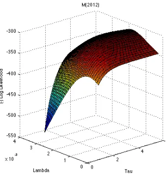
Cautious of such approach, we explored a fine search termination criteria of 0.0000001 and checked
if our estimates (⌧ and ) were robust for ¯K = 9,18,36. The estimates were found to be robust
and the log-likelihood function was observed to be concave (see Figure2), which suggest that our
estimates were indeed the global maximum.
Estimating the SK Model
The maximum likelihood technique involves ¯K+ 1 free parameters. We hence expressed p(a) as
p(a|↵0,↵1, ...,↵K¯, ) =p0↵0 ¯ K Y
k=1
pk(a| ,⌧)↵k
where↵k∈[0,1] denotes the proportion of Lk types in the data, given the constraints that ↵K¯ =
Figure 2: Cognitive Hierarchy Model Log-Likelihood Function for Session M(2012)
To ensure that our estimates are the global maximum, we considered multiple random starting
values for the parameters↵0,↵1, ...,↵K−¯ 1. Given this criteria, we repeated the estimation process
10 times for each session and the estimates were found to be identical each time. This suggest that