Multi jumps

Munich Personal RePEc Archive

Multi-jumps

Caporin, Massimiliano and Kolokolov, Aleksey and Renò,

Roberto

28 August 2014

Online at

https://mpra.ub.uni-muenchen.de/58175/

Multi-jumps

∗

Massimiliano Caporin

, Aleksey Kolokolov

and Roberto Ren`o

First draft: October 2013

This draft: August 28, 2014

Abstract

We provide clear-cut evidence for economically and statistically significant

mul-tivariate jumps (multi-jumps) occurring simultaneously in stock prices by using a

novel nonparametric test based on smoothed estimators of integrated variances.

Detecting multi-jumps in a panel of liquid stocks is more statistically powerful and

economically informative than the detection of univariate jumps in the market

in-dex. On the contrary of index jumps, multi-jumps can indeed be associated with

sudden and large increases of the variance risk-premium, and possess a statistically

significant forecasting power for future volatility and correlations which implies a

sizable deterioration in the diversification potential of asset allocation.

∗_{We thank Fulvio Corsi, Giampiero Gallo, Cecilia Mancini, Giovanna Nicodano, Francesco Ravazzolo,}

and the participants to the XV Workshop in Quantitative Finance (Florence, 2013) and at the 7th

Financial Risk International Forum in Paris (20-21 March, 2014), and the workshop Measuring and Modeling Financial Risk with High Frequency Data in Florence (19-20 June, 2014) for useful discussions. All errors and omissions are our own. The first author acknowledges financial support from the European Union, Seventh Framework Program FP7/2007-2013 under grant agreement SYRTO-SSH-2012-320270, and from Institute Europlace de Finance (EIF) under the research programSystemic Risk. The second author acknowledges financial support from the Riksbankens Jubileumsfond Grant Dnr: P13-1024:1 and the VR Grant Dnr: 340-2013-5180. The third author acknowledges financial support from Institute Europlace de Finance (EIF) under the research program A New Measure of Liquidity in Financial Markets.

†_{University of Padova, Department of Economics and Management,}

[email protected]

1

Introduction

Figure 1 shows the intraday log-returns of four financial stocks (see Table 6) on

Decem-ber, 11th _{2007. In that day, a FOMC meeting was taking place, ending with the decision}

of lowering the target for federal funds rate of 25 basis points, due to ”slowing economic

growth reflecting the intensification of the housing correction” and ”financial strains”1_.

The four financial companies collapsed all together in the afternoon, with a

contempora-neous log-return of approximately ₋3% which is clearly visible in the figure. The figure

also shows an evident increase, after the collapse, of both the stocks’ volatility and their

correlation. Moreover, the VIX index rose that day to 23.59 from 20.74 (+13.7%).

In the continuous time literature, a price movement of 3% (when the local volatility is

less than 0.5%, thus of more than six standard deviations in volatility units) is typically

modeled as a jump, that is a discontinuous variation of the price process. There are three

possible routes to the detection of collective events like that in Figure 1 in the data: i)

detection of a jump in a portfolio which includes the stocks (e.g., the equity index); ii)

detection of jumps in individual stocks; iii) direct detection of the multivariate jump (or

multi-jump as we call it in this paper). Surprisingly, a lot of effort has been devoted to

i) and ii), both theoretically and empirically, but almost none to iii). In this paper, we

introduce a formal test for the detection of multi-jumps, we argue that the third option is

actually the most effective and we show that it reveals additional economic information

which could not be revealed by the first two.

Multi-jumps are crucial events for asset allocation and risk management, as recognized

by the financial literature. For example, Longin and Solnik (2001) show that correlations

increase after a collective crash in the market, dampening the diversification potential of

portfolio managers, and Das and Uppal (2004) use multivariate jumps to model systemic

risk and its impact on portfolio choice. Bollerslev et al. (2008) use multi-jumps (common

1_{FOMC press release, December, 11}th_{2007, available at}

09:35 11:05 12:40 14:15 15:50 −3

−2.5 −2 −1.5 −1 −0.5 0 0.5 1

11−Dec−2007

Time

5−minutes returns (%)

BAC C JPM WFC

Figure 1: Intraday price changes (log-returns over 5 minutes) of Bank of America (BAC), Citigroup (C), JP Morgan (JPM) and Wells Fargo (WFC) on 11 December 2007. The four banking stocks collapse altogether around 14.15, while a FOMC meeting was taking place. We label this event a multi-jump. After the collapse, both volatility and correlation among stocks increases.

jumps, in their terminology) to explain jumps in the aggregated market index and discuss

that, for asset allocation, it is more important to be able to detect jumps occurring

simultaneously among a large number of assets, since the effect of co-jumps in a pair of

assets is negligible in a huge portfolio; Gilder et al. (2014) also study the relation between

common jumps and jumps in the market portfolio, and relate common jumps and news.

If rare, dramatic multi-jumps can be interpreted as systemic events carrying

market-wide information on economic fundamentals, their occurrence is also likely to affect the

aggregate attitude to risk and thus have an impact on risk premia. For example, Bollerslev

and Todorov (2011) empirically supported the view that risk compensation due to large

jumps is quite large and time-varying, while Drechsler and Yaron (2011) and Drechsler

(2013) highlight the importance of transient non-Gaussian shocks to fundamentals in

explaining the magnitude of risk premia. In this paper, we complement this evidence

by showing that multi-jumps can be associated with large increases in the variance risk

premium.

Despite the statistical, economic and financial importance of multi-jumps, the financial

their detection. A vast literature2 _{concentrated on univariate jump tests. Progress on}

developing tests for common jumps in a pair of asset prices was started by

Barndorff-Nielsen and Shephard (2003). They propose a way to separate out the continuous and

co-jump parts of quadratic covariation of a pair of asset prices. Mancini and Gobbi (2012)

developed an alternative threshold-based estimator of continuous covariation. Jacod and

Todorov (2009) proposed two tests for co-jumps, their approach relying on functionals

which depend, asymptotically, on co-jumps only. Finally, Bibinger and Winkelmann

(2013) develop a co-jumps test using spectral methods. However, these methodologies

apply to the case N = 2 only and their generalization to the case N > 2 is non-trivial.

Bollerslev et al. (2008) propose a test for common jumps in a large panel (N _{→ ∞})

which is based on the pairwise cross-product of intraday returns. In empirical work,

detection of multivariate jumps is typically achieved with a simple co-exceedance rule

(see, e.g., Gilder et al., 2014), according to which the multi-jump test is the intersection

of univariate tests.

We fill this gap in the literature by introducing a novel testing procedure for

multi-jumps which naturally applies to the caseN _≥2, withN finite. The proposed approach

builds on the comparison of two types of suitably introduced smoothed power variations.

High values of the test-statistics (which is asymptotically χ2_{(N) under the null) signal}

the presence of a multi-jump among at least M stocks, with M ≤ N. The smoothing

procedure depends on a bandwidth which can be used to approximately select the desired

M, with higher bandwidth values corresponding to higherM. We propose an automated

bandwidth selection procedure which can be tuned to get the desired M.

Using simulations of realistic price processes which accommodate for the most relevant

empirical features and which are implemented at the 5₋minutesfrequency (thus making

the testing procedure virtually immune from distortions due to the presence of

microstruc-ture noise), we show that the proposed procedure i) has desirable size properties; ii) is

2_{Barndorff-Nielsen and Shephard (2006); Lee and Mykland (2008); Jiang and Oomen (2008);}

more powerful and better sized than the Jacod and Todorov (2009) test, which needs a

much higher frequency (that is, many more data) to become effective; iii) is remarkably

powerful in detecting multi-jumps and iv) strongly outperforms the co-exceedance rule

in terms of power.

Results on real data are also encouraging. When applied to 16 liquid US stocks in the

pe-riod 2003-2012, the test reveals the significant presence of multi-jumps. Not surprisingly,

the multi-jumps occurrence rate becomes smaller with larger bandwidth, that is when we

increase the minimal orderM of stocks jumping jointly. However, multi-jumps with large

M (high bandwidth) are rare but important events, which can be always associated with

relevant market-wide economic news. This allows to interpret them as systemic events

affecting the market on a whole.

Importantly, detection of multi-jumps in the stocks reveals additional information with

respect to that conveyed by univariate jumps in the index. Indeed, while theoretically

a multi-jump in the constituents should always correspond to a jump in the index,

em-piricallythis is not necessarily true since the multi-jumps could have different directions

(even if empirical evidence reported in Section 5 documents that this is a quite unlikely

event: multi-jumps have typically the same direction) or they could occur in a small

sub-set of stocks, such that the jump in the index could be rather small and hard to detect.

These considerations are confirmed by the data: roughly a half of detected multi-jumps

in our sample cannot be associated with jumps in the index, unveiling information that

univariate jumps could not reveal.

The additional information conveyed by multi-jumps is economically significant. We

show that multi-jumps are strongly correlated with large increases in the variance risk

premium, while univariate jumps on the index are not. This result is in line with recent

theoretical literature, mentioned above, underscoring the impact of jumps in

fundamen-tals on changes in aggregate risk aversion, and the empirical result in Todorov (2010),

vari-ation in the variance risk-premium. When multi-jumps are used, the associvari-ation with

changes in the variance risk-premium becomes clear-cut also in our fully non-parametric

setting. This further indicates that multi-jumps are particularly suitable to test for

sys-temic events, while questioning the usage of index jumps via univariate statistics to this

purpose.

To further verify the potential empirical impact of multi-jumps, we show that they have

substantial predictive power for volatility and correlations. Both stock correlations and

volatilities are found to significantly increase after the occurrence of a multi-jump, thus

confirming, on a formal statistical ground, the anedoctical evidence in Figure 1. In

particular, the impact of multi-jumps on the correlation coefficient between a given pair

of stocks is quite strong, especially when compared to the impact of idiosyncratic co-jumps

between the same pair. These results have compelling implications for asset allocation.

A risk-averse investor who allocates her wealth in a portfolio of stocks and a risk-free

asset is harmed by the presence of multi-jumps in two ways. The first, which could be

dealt with the model developed by Das and Uppal (2004), is the change in the optimal

allocation strategy due to the presence of multi-jumps with respect to the case without

multi-jumps. The second, which we quantify here, is the impact of multi-jump on the

covariance matrix of the stocks, which implies an additional utility loss due to the increase

in the portfolio variance and the worsening of the diversification potential. The latter

effects would induce a less risky, that is less invested in stocks, optimal allocation strategy

than that recommended by traditional models.

The remainder of the paper is organized as follows. Section 2 describes the

continuous-time jump-diffusion model adopted in the paper. Section 3 explains the formal testing

procedure and provides asymptotic results. Section 4 presents results on simulated price

dynamics. Section 5 applies the test to real data and contains the empirical results and

2

Model

Denote the log-prices of an N-dimensional vector of assets byX = (X(i)₎

i=1,...,N. We

as-sume that stock prices evolve continuously on a filtered probability space (Ω,F,(F)t∈[0,T],P)

satisfying the usual conditions, and we assume the following dynamics for X,

accommo-dating for continuous (through Brownian motion) and discontinuous (through jumps)

shocks.

Assumption 1. X is an N-dimensional Ito semimartingale following:

dXt=atdt+ΣtdWt+dJt

where at (in RN) and Σt (in RN×M) are c`adl`ag adapted processes, Wt is standard

mul-tivariate Brownian motion in RM _{and J}

t is a finite activity jump process of the form

Jt(i) = PN_t(i)

k=1γ (i)

τ_k(i), i= 1, . . . , N, and N

(i)

t is a non-explosive counting process. Moreover,

we assume that the jump sizes are such that, ∀k = 1, . . ., we have P

γ(i)

τ_k(i) = 0

= 0,

i= 1, . . . , N.

The model, which is very general and encompasses virtually all parametric models

typi-cally used in financial applications, allows each component of X to include idiosyncratic

jumps (that occur only for a single stock) as well as common jumps among stocks. Define

the process

∆Xt=Xt−Xt−, (1)

and, as an example, consider the caseN = 3. The common jumps betweenX(1) _andX(2)

satisfy

∆Xt(1)∆X

(2)

t =γ

1(2)

t γ

2(1)

t ∆Nt12+γ

1(23)

t γ

2(13)

t ∆Nt123,

the three processes3 _satisfy

∆Xt(1)∆X

(2)

t ∆X

(3)

t =γ

1(23)

t γ

2(13)

t γ

3(21)

t ∆Nt123.

The inference procedure is designed to test the null

X

0≤t≤T

∆Xt(1)∆X

(2)

t ∆X

(3)

t = 0

against the alternative

X

0≤t≤T

∆X_t(1)∆X_t(2)∆X_t(3) ₆= 0.

Note that the presence of a multi-jump among three assets implies the presence of

co-jumps between each pair of them. However, the presence of co-co-jumps between each pair

of assets does not necessarily imply the presence of a multi-jump among them.

We do not explicitly include in the model market microstructure contaminations, since

the proposed method is thought to be applied at moderately low frequencies (e.g., five

minutes) where the impact of microstructure noise should be negligible. The theory

could however be easily extended to include market microstructure noise by adapting our

return smoothing technique to preaveraged estimators robust to both jumps and market

microstructure noise, as in Podolskij and Vetter (2009) and Hautsch and Podolskij (2013).

The theory could also be extended for infinite activity jumps (see, e.g., A¨ıt-Sahalia and

Jacod, 2012 and the references therein), since the test procedure developed below is based

on smoothed estimators of integrated variances which have been shown to be consistent

even in the presence of this kind of shock, see Mancini (2009) and Mancini and Gobbi

(2012).

3_{To underscore the methodological contribution of this paper, we use the word co-jump when the}

3

Multi-jumps inference

Assume to recordXin the interval [0, T], withT fixed, in the form ofn+1 equally spaced

observations4 _{and denote by ∆ =T /n. Define the evenly sampled logarithmic returns as}

∆jX =Xj∆−X(j−1)∆, j = 1, . . . , n. (2)

In order to formulate the statistical properties of the test, define the following sets:

ΩM J,N_T =_{ω_∈Ω _| the process

N Y

j=1

∆X(j)

t is not identically 0}

ΩNT = Ω\Ω M J,N T .

The set ΩM J,NT contains trajectories with common multi-jumps among all N assets in

[0, T]. The complementary set ΩN_T contains trajectories without multi-jumps inN stocks;

it could however contain jumps and multi-jumps up to N ₋1 stocks. Testing for

multi-jumps is equivalent to testing the following:

H0 :

(Xt(ω))t∈[0,T]∈Ω

N T

vs. H1 :

(Xt(ω))t∈[0,T]∈ΩM J,NT

. (3)

Inference is based on the definition of two newly defined integrated variance estimators

which constitute a generalization, particularly suitable to our application, of the truncated

realized variance estimator of Mancini (2009). To this purpose we need a definition of a

kernel and a bandwidth.

Assumption 2. A kernel is a function K(·) : R _→ R_{, which is differentiable with}

bounded first derivative almost everywhere in R_{, and such that K(0) = 1, 0≤ K(·) ≤1}

and limx→∞K(|x|) = 0. The bandwidth process is a sequence Ht,n of processes in RN

4_{This requirement can be easily generalized to non-equally spaced observations, if we set ¯∆ =}

maxi=1,...,n(ti−ti−1), whereti are observation times, and require ¯∆→0, see Remark i) of Theorem 4

which can be written as Ht,n =hnξt,n, where hn is a sequence such that

lim

n→∞hn = 0, nlim→∞

1 hn

r logn

n = 0, (4)

and ξt,n is a vector of N positive adapted stochastic process on [0, T] which are all a.s.

bounded with a strictly positive lower bound.

The bandwidth is written in the formhnξt,nto allow for data-dependent and time-varying

bandwidth. Indeed, in our application ξt,n is the local variance estimated by the

obser-vations themselves, see Eq. (31). We call hn the bandwidth parameter, and provide an

automated criterion for its selection in Section B.1 in the Appendix.

We now define two novel jump-robust integrated variance estimators, which are both

called Smoothed Realized Variance. The first one takes the form

SRV(X(i)_{) :=}

n X

j=1

∆jX(i) 2

·K ∆jX

(i)

H_j(_∆i)_,n !

, (5)

where X(i)_{, H}(i) _{are the i-th components of the vectors X, H and K(·) and H}

t,n are

the kernel and bandwidth defined in Assumption 2. This estimator coincides with the

estimator in Mancini (2009) when K(x) = I{|x|≤Ht,n}, but allows for a different choice

of the kernel. The intuition is however similar to that of Mancini (2009): ”smoothed”

squared returns ∆jX(i) 2

· K∆jX(i)/H

(i)

j∆,n

are close to squared returns ∆jX(i) 2

when they are small; smoothed squared returns are instead small when returns are large,

where the extent of ”largeness” is gauged by the bandwidth Hj∆,n. Asymptotically, this

procedure annihilates the jumps. The estimator of Mancini (2009) is the most draconian

in this respect, since using the indicator function implies that smoothed returns are zero

when returns are larger than Hj∆,n (dubbed threshold in Mancini’s terminology). The

advantage of replacing the indicator function with a smooth kernel is that it provides an

estimator which depends smoothly on the bandwidth: This stabilizes the procedure in

selection) and also eases bandwidth selection.

The following theorem (proof in Appendix A) shows that SRV(X(i)_{) in Eq. (5) is a}

jump-robust consistent estimator of integrated variance.

Theorem 3.1. Let the process X satisfy Assumption 1, and the kernel and bandwidth

satisfy Assumption 2. Then, as n → ∞ we have

SRV(X(i)₎ p

−→

Z T

0

(σ(i)₎2

udu, (6)

where σ(i) _{is the volatility of X}(i)

t .

The following remark introduce a correction to improve the estimator performance in

small samples.

Remark 1. (Small Sample Correction) In order to improve the finite samples

un-biasedness of the estimator defined in Eq. (5), it is advisable to normalize it as follows:

n X

j=1

∆jX(i)

2_·K ∆jX

(i)

H_j(_∆i)_,n !

∆

n X

j=1

K ∆jX

(i)

Hj(∆i),n

! −→p

Z T

0

(σ(i)₎2

udu,

since ∆Pn_j=1K

∆jX(i)

H_j(i_∆)_,n

p

−→1.

The second estimator takes the form:

g

SRVN_(X(i)_{) :=} n X

j=1

∆jX(i) 2

· K ∆jX

(i)

H_j(_∆i)_,n !

+

N Y

k=1

1−K ∆jX

(k)

H_j(k_∆)_,n

!!!

. (7)

Returns in Eq. (7) are smoothed as in Eq. (5), but they are also kept similar to the

original returns if all multivariate returns are big. Thus, even if, when n _{→ ∞}, both

smoothing procedures are meant to annihilate jumps, the smoothing in Eq. (7) will

Appendix A), which represents the base for inference and testing.

Theorem 3.2. Let the process X satisfy Assumption 1, and the kernel and bandwidth

satisfy Assumption 2. Then, as n _{→ ∞},

g

SRVN(X(i)₎ p

−→            RT

0 (σ (i)₎2

udu+

X

∆X_t(1)...∆X_t(N)6=0

∆Xt(i)

2

on ΩM J,NT

RT

0 (σ (i)₎2

udu, on Ω

N T

; (8)

where σ(i) _{is the volatility of X}(i)

t .

Theorems 3.1 and 3.2 introduce a natural estimator for the multi-jumps on each series.

By the light of Remark 1 the jump size of stock i corresponding to a multi-jump among

all stocks is naturally derived in the following remark.

Remark 2. (Multi-jump Size Estimation)

g

SRVN_(X(i)_)−SRV(X(i)₎

∆

n X

j=1

K ∆jX

(i)

H_j(_∆i)_,n

! −→p

           X

∆X_t(1)...∆X_t(N)6=0

∆Xt(i)

2

on ΩM J,N_T

0, on ΩNT

. (9)

In order to define the test statistics, we follow Podolskij and Ziggel (2010) and

de-fine a iid N × n matrix of draws (ηi

j)1≤i≤N,1≤j≤n, defined on the canonical extension

(Ω′,F′_,(F′₎

t∈[0,T],P′) of the original probability space (Ω,F,(F)t∈[0,T],P) and

indepen-dent from _F. We assume thatEηi j

= 1 andVarηi j

=Vη <∞. Define:

f

SV_(X(i)_{) :=} n X

j=1

∆jX(i) 2_·K

∆jX(i) Hj∆,n

·ηji, i= 1, . . . , N, (10)

and

SQ(X(i)_{) :=}

n X

j=1

∆jX(i) 4_·K2

∆jX(i) Hj∆,n

The test statistics is then defined as

S_n,N:= 1 Vη

N X

i=1

f

SV(X(i)_)−SRVgN_(X(i)₎2

SQ(X(i)₎ (12)

and its asymptotics is described in the following Theorem (proof in Appendix A).

Theorem 3.3. Under Assumption 1 and 2, if (ηi

j)1≤i≤N,1≤j≤n are pairwise independent,

as n → ∞, it holds: _

     

S_n,N−→d _χ2_{(N), on Ω}N

T

S_n,N−→p +∞ on ΩM J,N_T

; (13)

where χ2_{(N) denotes the χ-square distribution with N degrees of freedom.}

Theorem 3.3 implies that the statistic S_n,N can be used for testing for the presence of

multi-jumps. Under _H0, the value of Sn,N will be distributed as a χ2 with N degrees of

freedom. Under_H1, that is in the presence of multi-jumps, it will diverge as the number

of observations n increases.

Notice that the test defined in Eq. (12) is of computational orderN, in the sense that the

computational burden increases linearly with N. In particular, the test does not require

the estimation of the covariance between stocks (which would increase the computational

burden as N2_).

Following the suggestions of Podolskij and Ziggel (2010) for the univariate jump test, the

random variables ηi

j are allowed to take the values {1 +τ,1−τ} with equal probability,

so that Vη =τ2. In both Monte Carlo and empirical exercises we use τ = 0.05.

4

Simulation study

In order to simulate the dynamics of realistic prices, we simulate a multivariate model

idiosyncratic jumps and multi-jumps. All these components have been shown to be

present in the dynamics of high-frequency financial prices, and we use realistic parameter

values. We do not include market microstructure noise (see the discussion above). The

dynamics of the continuous parts of each component are given by the same stochastic

differential equations driven by correlated Brownian motions:

dXt(i) = µ dt+γtσt(i)dW

(i)

t +dJ

(i)

t

dlog(σt(i))2 = (α−βlog(σ

(i)

t )2)dt+ηdfW

(i)

t ,

(14)

wherei= 1, . . . ,16,W(i)_andWf(i)_{are standard Brownian motions with corrdW}(i)_{, dfW}(i)₌

e

ρ; σt(i) are stochastic volatility factors and γt represent intraday effects. The Brownian

motionsW(i) _{driving the price dynamics can be correlated, as specified below. The pure}

jump parts of X(i) _{are different compound Poisson processes.}

The parameters of the model are taken to be as estimated by Andersen et al. (2002) on

S&P500 prices: µ = 0.0304, α =₋0.012, β = 0.0145, η = 0.1153, ρ_e=₋0.6127; where

the parameters are expressed in daily units and returns are in percentage. The intraday

effects are given by:

γt =

1

0.1033(0.1271·t

2_{−0.1260·t+ 0.1239),}

as estimated on S&P500 intraday returns. In our simulations, we always have t_∈ [0,1],

with initial values for prices and volatility taken from the last simulated day.

The model (14) is discretized with the Euler scheme, using discretization step of ∆ = ₈₀1

which roughly corresponds to 5-minutes returns for a trading day of 6.5 hours (n = 80).

We generate samples of 1,000 days with different specifications for the jump processes

4.1

Two assets

We start with the case N = 2. The two assets are correlated, with

corr dW(1), dW(2)=ρ

with ρ= 0.5.

We generate different samples, subdivided into five categories. Jumps, when present,

come in the form of big jumps, with a size of 8p1/80, or small jumps, with a size of

4p1/80 (the average volatility in simulations being around 1). In the first category

(continuous processes), there are no generated jumps. In the second category (one big

jump) there are no co-jumps, but we generate a single big jump in the first component

X(1)_{, located randomly within the day. In the third category (big idiosyncratic jumps),}

bothX(1) _andX(2) _{have big jumps, but they are idiosyncratic in the sense that they never}

occur in the same time interval. The first three categories thus fall under the null. In the

fourth and firth categories (big co-jumpsand small co-jumps), which are the alternatives,

X(1) and X(2) contain one big-big and small-small co-jump respectively.

In this set of simulations, the S_n,N statistics are implemented using different bandwidth

parameters hn (see Section B.1 in the Appendix), namely hn = 5 and hn = 6.5 (see

Figure 9). For comparison, we also implement two co-jump tests proposed by Jacod and

Todorov (2009): Φj

n, which is used to test the null hypothesis of the presence of co-jumps,

and Φd

n, which is used to test the null of absence of co-jumps. The tests are described in

Section B.2 in the Appendix.

Table 1 analyzes the size properties for the three considered tests. Notice that the size of

S_n,N and Φn

d should be computed when co-jumps are absent, while the size of Φjn should

be evaluated when co-jumps are present. To underscore the dependence of the S_n,N on

the bandwidth, we denote it by S_n,N(hn). In the absence of jumps, both S80,2(5) and

jumps are added, size distortions appear, more strongly with lowerhn, and the distortions

are larger in the presence of two idiosyncratic jumps. In the case withhn= 6.5, however,

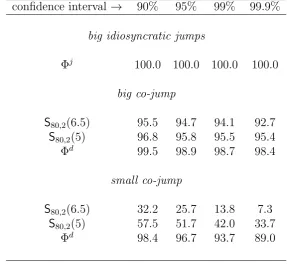
size distortions are reasonable: The simulated distribution of S_80,2(6.5), in the most

challenging case with big idiosyncratic jumps, is compared to its asymptotic limit in

Figure 2, top panel. On the other hand, the size of both Φj

n and Φdn is quite distorted.

This is not surprising, since also in Jacod and Todorov (2009) these tests have been shown

to need a much larger value of n to work properly.

Table 2 analyzes the power of the three tests. All the tests perform equally well when

co-jumps are big. When co-jumps are small they are obviously more difficult to detect.

The power of theS_80,2(6.5) increases with smallerhn, paralleling the corresponding larger

size distortions.

These results suggest that bandwidth selection can be used to trade-off size and power.

Higher bandwidth correspond to more reliable size but less power. In the case we are

testing for multi-jumps with largerN, this can be particularly useful, as we discuss below.

4.2

Four assets

We next proceed to simulate a system with N = 4. Continuous dynamics of all the

com-ponents is simulated as in equation (14), without jumps. The Brownian motions, driving

the first pair of components, are positively correlated: corr(W(1)_{, W}(2)_{) = 0.5. The}

sec-ond pair of components are negatively correlated: corr(W(3)_{, W}(4)_{) =−0.5. Correlations}

between the other pairs is null: corr(W(1)_{, W}(3)_{) =corr(W}(1)_{, W}(4)_{) = 0.}

In this set of simulations, we consider five cases:

1. Case 1: all components of X are continuous.

2. Case 2: all components of X contain a single big jump, but the four jumps occur

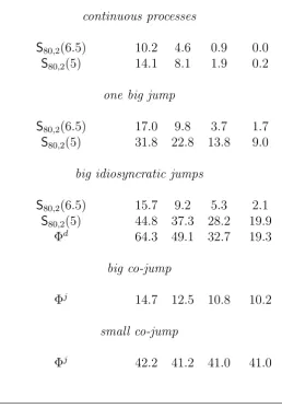
Table 1: Compares the size of competing tests in the case N = 2. Differ-ent processes for the null are considered. The sampling frequency is n= 80, corresponding to 5-minute intraday observations.

confidence interval → 90% 95% 99% 99.9%

continuous processes

S_80,2(6.5) 10.2 4.6 0.9 0.0

S_{80,2(5) 14.1 8.1 1.9 0.2}

one big jump

S_80,2(6.5) 17.0 9.8 3.7 1.7

S_80,2(5) 31.8 22.8 13.8 9.0

big idiosyncratic jumps

S_{80,2(6.5) 15.7 9.2 5.3 2.1}

S_80,2(5) 44.8 37.3 28.2 19.9

Φd _{64.3 49.1 32.7 19.3}

big co-jump

Φj _{14.7 12.5 10.8 10.2}

small co-jump

Φj _{42.2 41.2 41.0 41.0}

3. Case 3: there is a single multi-jump in the first triplet of the components ofX and

jumps are big.

4. Case 4: there is a multi-jump among the four processes and all jumps are small.

5. Case 5: there is a multi-jump among the four processes and all jumps are big.

Thus, Cases 1,2,3 represent the null and Cases 4,5 represent the alternative. The S_n,N

Table 2: Compares thepowerof competing tests in the caseN = 2. Different processes for the alternative are considerers. The sampling frequency isn= 80, corresponding to 5-minute intraday observations.

confidence interval → 90% 95% 99% 99.9%

big idiosyncratic jumps

Φj _{100.0 100.0 100.0 100.0}

big co-jump

S_{80,2(6.5) 95.5 94.7 94.1 92.7}

S_80,2(5) 96.8 95.8 95.5 95.4

Φd _{99.5 98.9 98.7 98.4}

small co-jump

S_{80,2(6.5) 32.2 25.7 13.8 7.3}

S_80,2(5) 57.5 51.7 42.0 33.7

Φd _{98.4 96.7 93.7 89.0}

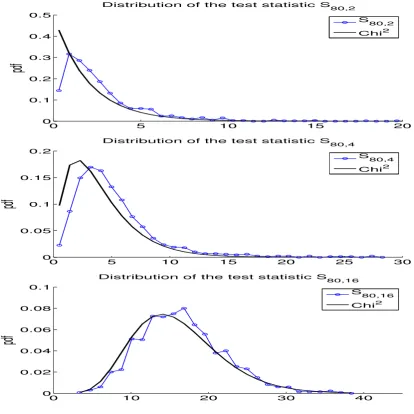
Table 3 shows the results for all Cases. With continuous processes and idiosyncratic

jumps, the size distortions (increasing with smaller hn, as before) are negligible. They

are instead quite strong against a multi-jump among M = 3 stocks with hn = 2.5,3.5.

The automated bandwidth selection indicates a value of hn = 5.5 in this case, and this

indeed provides a reasonable size (the distribution of the test in this case is compared to

the asymptotic limit in the middle panel of Figure 2). Power is practically unaffected by

the bandwidth if the multi-jump is composed of big jumps; while it decreases with higher

bandwidth if multi-jumps are small.

Again, the bandwidth parameter can thus be used to trade-off size and power.

Reason-able size can always be achieved, but at the obvious cost of less power. This opens an

interesting possibility for the econometrician. The null (no multi-jumps acrossN assets)

0 5 10 15 20 0

0.1 0.2 0.3 0.4 0.5

pdf

Distribution of the test statistic S_80,2

S_80,2

Chi2

0 5 10 15 20 25 30

0 0.05 0.1 0.15 0.2

pdf

Distribution of the test statistic S

80,4

S_80,4

Chi2

0 10 20 30 40

0 0.02 0.04 0.06 0.08 0.1

pdf

Distribution of the test statistic S_80,16

S_80,16 Chi2

Figure 2: Shows the simulated distribution of the proposed multi-jump tests together with its asymptotic distribution under the null (which isχ2_{(N)); the}

tests are S80,2(6.5) for N = 2 in the case with big idiosyncratic jumps (top

panel),S80,4(5.5) forN = 4 in Case 3 (center panel) andS80,16(4.5) forN = 16

in Case 3 (bottom panel).

could consider several alternatives when computing the test on N assets: multi-jump in

N assets, in N −1 assets, in N −2 assets and so on. The bandwidth parameter can

be used to disentangle these cases. For example, looking at Table 3, we see that with

hn = 5.5 we would disentangle a multi-jump in 4 stocks by a multi-jump in 3 stocks; with

hn = 3.5 we would also detect multi-jumps in three stocks, and with hn = 2.5 we would

also detect multi-jumps in two stocks. In empirical work, the choice of hn could depend

Table 3: Shows thesize andpower of the proposed test in the caseN = 4. Different processes under the null and the alternative are considered. The sampling frequencyn= 80 corresponds to 5-minute intraday observations.

confidence interval → 90% 95% 99% 99.9%

Case 1: continuous processes

S_80,4(2.5) 12.3 6.2 1.6 0.1

S_{80,4(3.5) 9.9 4.1 0.6 0.1}

S_80,4(5.5) 11.1 5.1 0.7 0.0

Case 2: big idiosyncratic jumps

S_80,4(2.5) 14.0 7.7 3.1 1.4

S_{80,4(3.5) 8.6 4.3 0.4 0.0}

S_80,4(5.5) 5.7 1.8 0.1 0.0

Case 3: multi-jump in N = 3 stocks

S_80,4(2.5) 71.8 68.6 63.6 61.3

S_{80,4(3.5) 55.8 50.9 45.1 41.1}

S_80,4(5.5) 14.0 9.3 3.6 2.1

Case 4: small multi-jump

S_80,4(2.5) 94.2 92.9 90.4 87.2

S_{80,4(3.5) 53.2 46.9 37.5 30.4}

S_80,4(5.5) 10.2 4.8 0.9 0.2

Case 5: big multi-jump

S_80,4(2.5) 98.7 98.7 98.6 98.6

S_{80,4(3.5) 98.8 98.7 98.6 98.6}

S_80,4(5.5) 98.2 98.0 97.5 96.7

4.3

Many assets

We finally simulate a large number of stocks, that isN = 16 as in the empirical application

below. Continuous parts of all components follow equation (14). The Brownian motions

the stock returns used in the empirical application in Section 5. We now consider the

following settings:

1. Case 1: all components of X are continuous.

2. Case 2: there is a multi-jump in M = 4 components of X with big jumps.

3. Case 3: there is a multi-jump in M = 15 components of X with big jumps.

4. Case 4: there is a multi-jump in M =N = 16 components of X and all jumps are

small.

5. Case 5: there is a multi-jump in M =N = 16 components of X and all jumps are

big.

In this setting, Cases 1,2,3 represent the null and Cases 4,5 two possible alternatives.

Here we implement S_n,N-test with hn= 1,2,4.5 (see Figure 9). The bandwidth hn = 4.5

is selected by our automated bandwidth selection method under a null with M = 15

multi-jumps.

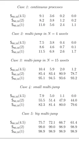
Table 4 shows the results. For all the considered bandwidth, size is reasonable in the

case of continuous processes and moderate multi-jump (M = 4), but becomes distorted

in the case M = 15 unless we use the automatically selected value hn= 4.5. This result

is in line with the simulation evidence presented above; size is more reliable with higher

bandwidth, while power is instead higher with lower bandwidth. The econometrician

should then choosehn= 4.5 if he is interested in multi-jumps among 16 jumpsonly. This

will somewhat sacrifice power. If instead one is interested in multi-jumps across fewer

stocks, a smaller hn can be used; for example, with hn = 2 we are still robust against

moderate multi-jumps across M = 4 stocks, but we would detect most of the

multi-jumps with M = 15 too (and, with decreasing power, with M = 14,13, . . .) also when

their magnitude is modest. This feature of the test is actually very appealing, especially

with a very large N, and indeed in our empirical application we take advantage of it by

Table 4: Shows thesizeandpowerof the proposed test in the caseN = 16. Different processes under the null and the alternative are considered. The sampling frequencyn= 80 corresponds to 5-minute intraday observations.

confidence interval → 90% 95% 99% 99.9%

Case 1: continuous processes

S_80,16(4.5) 9.1 3.6 0.2 0.0

S_{80,16(2) 8.2 3.8 1.2 0.2}

S_80,16(1) 11.0 5.6 2.4 1.1

Case 2: multi-jump in N = 4 assets

S_80,16(4.5) 7.5 3.8 0.4 0.0

S_{80,16(2) 8.6 4.6 0.7 0.1}

S_80,16(1) 11.5 6.8 2.6 1.7

Case 3: multi-jump in N = 15 assets

S_80,16(4.5) 10.4 5.9 2.0 1.2

S_{80,16(2) 85.4 83.4 80.9 78.7}

S_80,16(1) 95.1 94.5 93.6 93.2

Case 4: small multi-jump

S_80,16(4.5) 7.9 5.0 1.1 0.0

S_{80,16(2) 55.5 51.4 47.9 44.0}

S_80,16(1) 82.3 81.4 80.0 79.6

Case 5: big multi-jump

S_80,16(4.5) 75.7 72.1 66.7 61.4

S_{80,16(2) 99.0 99.0 98.9 98.9}

S_80,16(1) 98.9 98.9 98.9 98.9

Summarizing, our simulation experiments indicate that the bandwidth parameter, which

trades off size and power, can always be set (with an automated procedure) to get correct

size and reasonable power. Moreover, by tuning the bandwidth parameter the test can

be sensibly used to detect multi-jumps with a given maximum order M, up to the total

4.4

Comparison with univariate tests

An alternative way to test for multi-jumps is the intersection of univariate test, also named

co-exceedance rule, as in Gilder et al. (2014). In this section we show, with simulated

data, that the new multi-jump test proposed in this paper is much more powerful than

the intersection of univariate tests.

We state the co-exceedance rule as follows: reject the absence of multi-jumps in the N

-dimensional price vector if the absence of jumps is rejected (based on a univariate jump

test) for each component. We compare three univariate jump tests: the CPR test of

Corsi et al. (2010), the BNS test of Barndorff-Nielsen and Shephard (2006) and the ABD

test of Andersen, Bollerslev and Dobrev (2007), all described in Appendix B.2.

We simulate 1,000 paths ofN = 16 stocks, with the continuous part as in subsection 4.3.

Each path contains a single multi-jump across the 16 stocks, with jump sizes normally

distributed with mean being equal to 8√∆ and standard deviation 2√∆. Hence, jump

sizes are sufficiently large on average, but show dispersion such that some of the univariate

jumps might be smaller (we recall that the continuous daily variance hovers around 1).

Table 5 shows size and power for univariate jump tests and multi-jump tests based on the

S_{n,N statistics and the co-exceedance rule. For univariate tests, we confirm the findings in}

the literature (see Dumitru and Urga, 2012 for a wider comparison). The most powerful

test is ABD, but at the cost of a distorted size. CPR and BNS are correctly sized, but

CPR has higher power, thus striking a superior balance. For this reason, we mainly use

CPR for detecting univariate jumps in the empirical application in Section 5.

For multi-jump test, theS_n,Nproposed here is much more powerful than the co-exceedance

rule. The intersection of CPR would miss nearly 75% true multi-jumps at the 95%

confidence level; the intersection of ABD misses only 34% at the same confidence level,

but just because its size is distorted. This is not totally surprising: the co-exceedance rule

Table 5: Shows thesizeandpowerof the proposed test in comparison with the co-exceedance rule, for the caseN= 16, and for univariate jump tests. The size is computed under the assumption of continuous processes. The sampling frequencyn= 80 corresponds to 5-minute intraday observations.

confidence interval → 90% 95% 99% 99.9%

Multi-jump tests: power

S_80,16(2) 98.6 98.5 98.5 98.4

T16

i=1CP R 32.7 25.1 9.1 1.8

T16

i=1BN S 14.2 7.9 1.5 0.0

T16

i=1ABD 71.8 66.0 53.7 37.1

Univariate tests on individual stocks: power

CP R 91.2 89.0 84.4 73.9

BN S 86.0 81.9 71.5 56.1

ABD 97.0 96.6 95.1 92.8

Multi-jump tests: size

S_80,16(2) 7.7 2.6 0.3 0.0

Univariate tests on individual stocks: size

CP R 9.2 5.3 2.1 0.0

BN S 8.6 4.8 1.9 0.0

ABD 17.3 10.8 3.0 0.8

cost of increasing spurious detection of univariate jumps. The size of the S_n,N, computed

on a multi-variate process without jumps, is again reasonably correct. The size of the

intersection tests cannot be reported since the distribution under the null is unknown.

It is also interesting to note that the S_{n,N can be conveniently used as a preliminary}

tool in a two-steps procedure to detect days with jumps in the first step, and then

complemented by univariate tests, applied singularly to each stock, in the second step.

Moreover, S_n,N can be much more effective in detecting univariate jumps (which could

they are synchronous. Indeed, the power ofS_n,N declines at a much slower rate than the

power of univariate tests when increasing the confidence interval. After all, many jumps

are better seen than only one.

These considerations can be important for empirical studies, since jumps (and

multi-jumps) are rare events. For example, with N = 2,000 days, testing against a jump

arrival rate of 2% per day using CPR at 99% confidence interval, we expect (based

on figures in Table 5) to detect 35.8 true jumps (out of 40) and 20 spurious jumps,

which would jeopardize empirical work based on these measures. For this reason, very

large confidence intervals (such as 99.9% or 99.99%) are tipically used in practice. With

confidence intervals so selective, the S_n,N could be an effective companion tool for jump

detection, which is certainly more effective if these jumps are actually multi-jumps. This

can be especially important when detecting jumps in large portfolios, like the stock index,

as we further discuss in Section 5.

To summarize, the results in this subsection show that the co-exceedance rule is not

accurate, even when it is based on relatively powerful univariate tests, while the

multi-jumpS_n,Ntest proposed here is powerful and accurate, thus indicating a strong preference

for the latter in empirical work. We point out that such a feature would be crucial in

a number of applications, for instance when dealing with the identification of systemic

multi-jumps.

5

Empirical application

The data set we use for the empirical application is the collection of N = 16 blue chip

stocks quoted on the New York Stock Exchange and belonging to four different economic

sectors, and of the S&P500 index. The stocks and the corresponding ticker are listed in

Table 6. The data were recovered from the TickData One Minute Equity Data (OMED)

Table 6: Reports the list of the sixteen blue chip stocks used in the empirical application, their ticker and the estimated β computed with respect to the S&P500 index and used in the asset allocation exercise in Section 5.5.

Company Ticker β

Bank of America BAC 1.77 Citigroup Inc. C 1.70 JPMorgan Chase & Co. JPM 1.60 Wells Fargo & Company WFC 1.52

Boeing BA 0.95

Caterpillar Inc. CAT 1.18 FedEx Corporation FDX 1.02 Honeywell International Inc. HON 1.03 Hewlett-Packard Company HPQ 0.79 International Business Machines Corp. IBM 0.93 AT&T Inc. T 1.05 Texas Instruments Incorporated TXN 0.82 Kraft Foods Inc. KFT 0.57 PepsiCo, Inc. PEP 0.55 The Procter & Gamble Company PG 0.56 Time Warner Inc. TWX 1.05

went trough a standard filtering procedure. TickData one-minute equity data are adjusted

for corporate actions such as mergers and acquisitions or symbol changes. Moreover, the

underlying tick data used to build 1-minute time series are first controlled for cancelled

trades, or records not temporally aligned with previous/subsequent data; then filtered to

identify bad ticks which are corrected using validation with third-party sources.

In our empirical application, we use returns at the 5-minutes frequency, corresponding to

n = 77 intraday returns. This frequency represents a tradeoff between achieving enough

statistical power and avoiding distortions which could potentially arise from

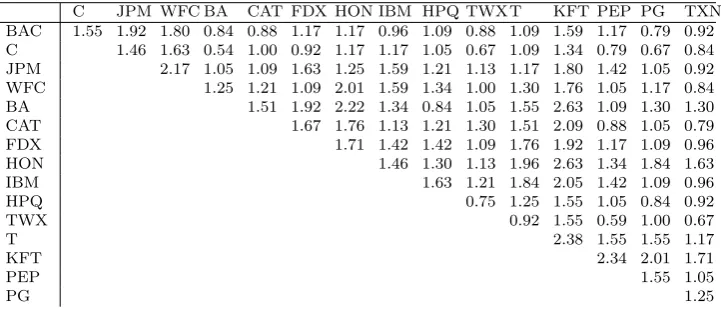
Table 7: Reports the frequencies of rejections (in percentage) for the null hypothesis of absence of co-jumps between stock pairs (that is, the percentage of days with co-jumps), tested with the proposed multi-jump testS77,2(6.5) at

0.1% confidence level. The global average of rejections among pairs is 1.33%.

C JPM WFC BA CAT FDX HON IBM HPQ TWXT KFT PEP PG TXN

BAC 1.55 1.92 1.80 0.84 0.88 1.17 1.17 0.96 1.09 0.88 1.09 1.59 1.17 0.79 0.92 C 1.46 1.63 0.54 1.00 0.92 1.17 1.17 1.05 0.67 1.09 1.34 0.79 0.67 0.84 JPM 2.17 1.05 1.09 1.63 1.25 1.59 1.21 1.13 1.17 1.80 1.42 1.05 0.92 WFC 1.25 1.21 1.09 2.01 1.59 1.34 1.00 1.30 1.76 1.05 1.17 0.84

BA 1.51 1.92 2.22 1.34 0.84 1.05 1.55 2.63 1.09 1.30 1.30

CAT 1.67 1.76 1.13 1.21 1.30 1.51 2.09 0.88 1.05 0.79

FDX 1.71 1.42 1.42 1.09 1.76 1.92 1.17 1.09 0.96

HON 1.46 1.30 1.13 1.96 2.63 1.34 1.84 1.63

IBM 1.63 1.21 1.84 2.05 1.42 1.09 0.96

HPQ 0.75 1.25 1.55 1.05 0.84 0.92

TWX 0.92 1.55 0.59 1.00 0.67

T 2.38 1.55 1.55 1.17

KFT 2.34 2.01 1.71

PEP 1.55 1.05

PG 1.25

5.1

Multi-jumps in the market

We start by applying the co-jumps test (N = 2) for all the 120 pairs throughout all the

sample. Table 7 reports the percentage of rejections of the null at the 99.9% confidence

level for all pairs. Co-jumps are significant events. On average (among pairs), we detect

co-jumps in 1.33% of days. The low probability of co-jumps is in line with other existing

empirical work (see, e.g., Table III of Lahaye et al., 2011 for stock indexes and FX rates).

The co-jumps are distributed quite uniformly among stock pairs. The maximum amount

of rejections is obtained between HON and KFT (2.63%), while the minimum is observed

between C and BA (0.54%).

We then detect multi-jumps among all 16 stocks using a confidence interval 1−α such

that the expected number of spurious detection in the sample is 0.1 asymptotically, that

is α = 4.18_·10−5_{. We are thus looking for solid rejection of the null, that is strong}

signals and virtually no false positives. We use bandwidth parametershn between 1 and

3. As documented in the simulation study, the higher bandwidth hn= 3 corresponds to

more correct size against the null of absence of multi-jumps inallthe 16 stocks, meaning

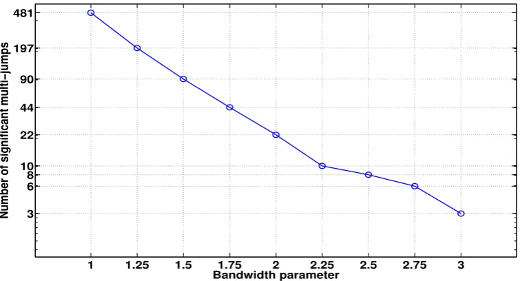
1 1.25 1.5 1.75 2 2.25 2.5 2.75 3 3

6 8 10 22 44 90 197 481

Bandwidth parameter

Number of significant multi−jumps

Figure 3: Reports the number of multi-jumps detected by the test introduced in Section 3. The test outcome is reported for different bandwidth parameters. The smaller bandwidthhn= 1 corresponds to the detection of at leastM ≃5

multi-jumps. The larger bandwidth hn= 3 corresponds to the detection of at

leastM _≃15 multi-jumps.

certainly too stringent for empirical analysis. Table 4 shows instead that, with the lower

bandwidth hn = 1, the test is reasonably sized against the contemporaneous presence of

M = 4 multi-jumps (at least). Thus, we interpret the rejection of the null with 1≤hn≤3

as a signal for the presence of a significant multi-jumps in at leastM stocks, withM ≈5

for hn = 1 and M ≈ 13 for hn = 2 (see Figure 9). In the case hn = 2, therefore, the

multi-jump would involve all the four economic sectors.

Figure 3 reports the number of detected multi-jumps corresponding to different

band-widths. Their number vary from 481 (20.1% of the sample) at hn = 1 to just 3 (0.13%

of the sample) at hn = 3. Thus, multi-jumps are largely statistically significant in our

sample, but multi-jumps across many stocks are rare events.

However, these rare events are strongly economically significant. Table 8 reports the dates

of the 22 multi-jumps detected with hn = 2, and associates macroeconomic/financial

information to each date; it also reports the corresponding VIX daily changes, SP500

Table 8: Multi-jump dates (when the test is implemented withhn= 2, that is

with approximately more thanM _≃13 multi-jumps) are listed together with i) multi-jump direction, ii) percentage change in S&P500, iii) percentage volume change, iv) VIX difference and v) economic/financial events occurred on those days.

date Multi-jump

direction

SP500 change (%)

Volume change (%)

VIX change

Economic/Financial events

25-Jun-2003 negative −0.83 +1.81 +0.06 FOMC meeting cuts federal fund rate of 25bps

18-Apr-2006 positive +1.71 +35.19 −1.18 Release of minutes of FOMC meet-ing of 27-28 Mar

08-Aug-2006 negative −0.34 +29.23 −0.00 FOMC keeps its target for the fed-eral funds rates

18-Sep-2007 positive +2.92 +30.98 −6.13 FOMC lowers its target for the fed-eral funds rates by 50 bps

25-Feb-2008 positive +1.38 −5.74 −1.03 FED Term Auction Facility 16-Jul-2008 positive +2.51 +4.70 −3.44 Release of minutes of FOMC

meet-ing of 24-25 Jun

29-Sep-2008 negative −8.81 +15.37 +11.98 FOMC meeting unscheduled 10-Feb-2009 negative −4.91 +29.58 +3.03 U.S. Treasury Secretary Geithner

announces a Financial Stability Plan 17-Feb-2009 both −4.56 +20.10 +5.73 27-28 FOMC minutes released on

Feb 18

23-Feb-2010 negative −1.21 +14.80 +1.43 FED releases minutes of its discount rate meeting on January 25, 2010. 06-May-2010 negative −3.24 +49.28 +7.89 The Flash Crash

28-May-2010 negative −1.24 −7.66 +2.39 FED announces three small auctions through the Term Deposit Facility 01-Sep-2010 positive +2.95 +13.44 −2.16 Release of minutes of FOMC

meet-ing of 27-28 Mar (Aug 31) 23-Jun-2011 positive −0.28 +32.84 +0.77 FOMC meetings (21 and 22 June) 01-Jul-2011 positive +1.44 −34.12 −0.65 Arab Spring starts

01-Aug-2011 negative −0.41 −2.19 −1.59 Unscheduled FOMC meeting 01-Sep-2011 positive −1.19 −18.67 +0.20 Release of minutes of FOMC

meet-ing of 27-28 Mar (Aug 30)

31-Oct-2011 negative −2.47 −7.49 +5.43 FOMC committee scheduled for 1-2 November

23-Nov-2011 negative −2.21 −3.50 +2.01 Release of the minutes of the FOMC committee of 1-2 November 28-Nov-2011 positive +2.92 +50.79 −2.34 FOMC meeting unscheduled 03-Apr-2012 negative −0.40 +7.99 +0.02 13 March FOMC minutes released 14-Jun-2012 positive +1.08 −3.91 −2.59 Federal Reserve Board issues

en-forcement actions

see that almost all the multi-jumps in the Table can be easily associated with impactful

economic news, mainly related to FED activity, more prominently FOMC meetings, but

also important financial and global news. Moreover, the traded volume tends to be

considerably higher (than the previous day) on days in which a multi-jump occurs. The

VIX index tends to move, in multi-jump days, in an opposite direction with respect to

the market, as also noticed in Todorov and Tauchen (2010). Below we provide formal

statistical evidence of a significant increase of the variance premium associated with

Multi-jumps are also typically, but not always, associated with jumps in the S&P 500

stock index. We use three tests for detecting jumps in the stock index: the ABD test,

the BNS test and the CPR test (see Appendix B.2 for their description) at the 99.9%

confidence interval. The left panel of Table 9 reports the percentage of cases in which,

in a day with a multi-jump, we also detect a jump in the index. We can see that testing

for jumps in the index results in a significant information loss with respect to testing for

multi-jumps. The test with the highest overlap is ABD, which however is also the test

with largest size distortions (that is, with supposedly more false positives).

The fact that decreasing the bandwidth parameter we have less overlap between

multi-jumps and multi-jumps in the index is not surprising: multi-jumps in the index are easier to detect

in the presence of multi-jumps among more constituents. The fact that jumps in the

stock index are not detected in all multi-jump days deserves further investigation. This

could be due to a subset effect (only the 16 stocks considered here jumped, but not the

other index constituents) or to a power effect (if the univariate tests on the index are

less powerful than the multi-jump test). To shed light on this issue, we also compute the

univariate jump tests on the equally weighted portfolio of the sixteen stocks (right panel

of Table 9), thus eliminating the subset effect. We can indeed observe a slight increase of

the performance of CPR and ABD tests, but not such to fill the gap with the multi-jump

test. The performance of BNS on the equally weighted portfolio is even worst. This result

demonstrates that the power effect is dominant: a multi-jump in the 16 stocks certainly

implies a jump in their portfolio, which however the univariate tests are often unable to

detect. The problem is very severe for the BNS test, whose performance is particularly

poor. These results altogether suggests that it is significantly more powerful to test for

multi-jumps among stocks than for jumps in a portfolio. The next sections also show

that the additional information carried by the multi-jump test, which cannot be revealed

by univariate jump tests, is economically significant.

Finally, most jumps in the index can be associated to multi-jumps in the stocks: using

Multi-jumps and jumps in the S&P 500 index

hn= 2 hn = 1.5 hn= 1

CPR 59.1% 43.2% 33.3% BNS 40.9% 25.0% 16.7% ABD 81.8% 63.6% 58.9%

Multi-jumps and jumps in the equally weighted portfolio

hn= 2 hn= 1.5 hn = 1

CPR 68.2% 54.5% 40.0% BNS 36.4% 22.7% 13.3% ABD 90.9% 75.0% 64.4%

Table 9: Reports the percentage of days with a detected multi-jumps (accord-ing to the bandwidth parametershn = 2,1.5,1) in which we also detect a jump

in the S&P500 index (left panel) and in the equally weighted portfolio of the 16 stocks (right panel) according to three different jump tests at the 99.9% confidence interval. Testing for a jump in the portfolio is less powerful than testing for multi-jumps among constituents.

Of these jumps, 77 correspond to days in which there is a multi-jump withhn≥1. Thus,

jumps in the index can be typically (but not always) associated with multi-jumps in its

most liquid constituents. The remaining jumps in the index could be explained by jumps

in a subset of constituents with not enough overlap with the stocks considered here, or

by size distortions larger than what predicted by our simulated data.

5.2

Jumps, multi-jumps and the variance risk premium

This section shows the relevance of detecting multi-jumps in the data (with respect to

jumps in the index) by associating their occurrence to changes in the variance risk

pre-mium. The variance risk premium on day t for a given maturity τ is defined as:

V RPt =QVQ(t, t+τ)−QV(t, t+τ) (15)

where QVQ_{(t, t+τ) is the risk-neutral quadratic variation of the stock index between}

times tand t+τ, andQV(t, t+τ) is the actual quadratic variation in the same interval.

showing that V RPt carries significant forecasting power for future returns; see also Carr

and Wu (2009); Bollerslev and Todorov (2011). We use τ = 1 month and we estimate

V RPt in our sample using:

\

V RPt=V IXt,t2+30−RVgt,t+30 (16)

where V IXt,t+30 is the 30-days VIX index computed by CBOE, that is the model-free

implied volatility (Jiang and Tian, 2005), andRVgt,t+30is the forecasted realized variance

in the same period obtained with the regression:

logRVt,t+30=α1+α2logRVt−30,t−1 +α3logRVt−90,t−1+εt, (17)

where εt is iid noise and

RVt,t+h = 252·ψ· X

t≤t′_≤t+h

RV_t′,

with RV_t′ being the 5-minutes open-to-close realized variance on day t, properly rescaled

by 252 (to convert it to yearly units) and by the constant ψ, which is the ratio between

the sum of squared close-to-close S&P500 daily returns and the average of RV in the

sample, and which is meant to take into account the contribution of overnight returns to

the total variance.

The time series of the estimated variance risk premium in our sample is shown in Figure

4. As expected from the theory, it is almost always positive. We associate it to jumps

in the stock market index (S&P500) and multi-jumps in the sample of sixteen stocks, by

using the following regression models, in which the variance risk premium is driven by

an autoregressive process and by dummy variables for jumps,

[

V RPt=γ0+γ1V RP[t−1+γJeJt+γM JM Jgt+γM J− M Jgt·I{rSP

2003 2004 2005 2006 2007 2008 2009 2010 2011 2012 2013 −2000

−1000 0 1000 2000 3000 4000

Variance Risk Premium

Figure 4: Reports the daily estimated variance risk premium, computed as in equation (16), for the available sample.

where t denotes the day,eJ_t is an indicator function signaling jump in S&P500 index (we

use the CPR test at 99.9% confidence level),M Jgtis an indicator function for the presence

of a multi-jump (withhn= 2, 1.75 and 1.5), I{rSP

t <0} is an indicator function fornegative

close-to-close return on S&P500 on dayt and ǫt are iid shocks with zero mean and finite

variance.

We also run the same regression with lagged dummy variables, that is with eJ_{t →} eJ_t−1, g

M Jt →M Jgt−1 andI{rSP

t <0} →I{rSPt−1<0}, to examine the predictive power of multi-jumps on the variance risk premium. Estimation results, adjusted with the standard Newey and

West correction, are presented in Table 10 for various restrictions and multi-jump test

bandwidth parameters.

We find that the constant γ0 and the auto-regressive coefficient γ1 are strongly

signifi-cant. More importantly, our results show that the occurrence of jumps in the index is

insignificant (or mildly negative) when regressed together with variance premium, and

thus cannot be associated to it. On the contrary, multi-jumps are significant and have a

strong impact, especially when they contribute to a market downturn. When the

Table 10: Estimates (Newey-West corrected) of model (18) with different restrictions and different choices of the multi-jump dummy. T-statistics are in parenthesis. Top panel: regression with contemporaneous dummies. Bottom panel: regression with lagged dummies. One star denotes 90%, two star 95% and three stars 99% significance.

Contemporaneous regressions

γ0 31.7∗∗∗ 31∗∗∗ 30.3∗∗∗ 30.2∗∗∗ 31.5∗∗∗ 30.7∗∗∗ 30.1∗∗∗ 28.8∗∗∗ 31.3∗∗∗ 31.3∗∗∗ (5.18) (5.2) (5.17) (5.17) (5.18) (5.16) (5.1) (4.97) (5.15) (5.14) γ1 0.836∗∗∗ 0.835∗∗∗ 0.833∗∗∗ 0.832∗∗∗ 0.835∗∗∗ 0.835∗∗∗ 0.832∗∗∗ 0.83∗∗∗ 0.835∗∗∗ 0.835∗∗∗

(24) (24.1) (23.8) (23.6) (24) (24.1) (23.7) (23.7) (24) (24)

γJ −0.41 −8.15 −8.52 −4.67

(-0.0491)

(-0.881)

(-0.98) (-0.534)

γM J 89.3 93.9∗ −96∗∗∗

(hn= 2) (1.64) (1.68) (-2.94)

γM J 104∗∗∗

(hn= 1.75) (2.75)

γM J 60.6∗

(hn= 1.5) (1.86)

γ−

M J 184∗∗∗ 188∗∗∗ 282∗∗∗

(hn= 2) (2.75) (2.78) (3.85)

γ−

M J 193∗∗∗

(hn= 1.75) (3.82)

γ−

M J 176∗∗∗

(hn= 1.5) (3.81)

Lagged regressions

γ0 32.2∗∗∗ 31.5∗∗∗ 31.6∗∗∗ 30.5∗∗∗ 32.2∗∗∗ 31.5∗∗∗ 31.7∗∗∗ 31.4∗∗∗ 32.2∗∗∗ 32.2∗∗∗ (5.3) (5.27) (5.25) (5.2) (5.3) (5.27) (5.27) (5.25) (5.31) (5.31) γ1 0.835∗∗∗ 0.835∗∗∗ 0.835∗∗∗ 0.831∗∗∗ 0.835∗∗∗ 0.835∗∗∗ 0.836∗∗∗ 0.834∗∗∗ 0.834∗∗∗ 0.834∗∗∗

(24) (24) (24) (23.5) (24) (23.9) (23.9) (23.6) (23.9) (23.9)

γJ −7.44 −10.8∗ −10.5∗ −9.66∗

(-1.48) (-1.79) (-1.92) (-1.71)

γM J 34.5 40.6 −22.5∗∗∗

(hn= 2) (0.804) (0.91) (-2.58)

γM J 4.07

(hn= 1.75) (0.0728)

γM J 51.8

(hn= 1.5) (1.34)

γ−

M J 67 71.7 93.8

(hn= 2) (1.07) (1.13) (1.52)

γ−

M J 2.49

(hn= 1.75) (0.0303)

γ−

M J 29.4

of contemporaneous multi-jumps ranges from 60.6 to 104 points, and from 176 to 193

points when associated with negative S&P500 returns. This is substantial, since the

av-erage variance risk premium in our sample is equal to 193.6. This means that variance

premium almost doubles (on average) in days with a multi-jump and a downturn of the

market. The effect of downward multi-jump is so strong that it subsides the effect of

jumps and overall multi-jump, the latter becoming significantly negative in the

encom-passing regression (last column of Table 10) indicating that positive multi-jump have the

opposite effect on the variance risk premium.

Summarizing, multi-jumps, and precisely negative ones, can be associated with a

signif-icant increase in the variance risk premium, while index jumps cannot. The inability of

jumps in capturing variance risk premia changes might depend on the documented

in-adequacy of nonparametric univariate tests in capturing economically significant jumps.

From a theoretical point of view, our finding corroborates the view that non-Gaussian

shocks to fundamentals (sometimes referred to as disasters) have a substantial impact

on risk premia, see e.g. Barro (2006); Gabaix (2012) and Drechsler and Yaron (2011);

Drechsler (2013) for economic models directly focusing on the relation between jumps in

fundamentals and the variance risk premium. From this theoretical perspective, the

ab-sence of correlation between jumps in the stock market index and variance risk premium

changes is rather puzzling. Indeed, also Todorov (2010) shows a strong link between

index jump measures and variance risk premium changes through the estimation of a

parametric model.5 _{This paper documents that this puzzle is due to the relatively low}

power of univariate jump tests to detect systemic market events affecting fundamental

value, and that this shortcoming can be overcome by testing for multi-jumps in a (not

very large, but economically representative) stock panel.

5_{In his preliminary analysis, Todorov (2010) also reports a significant correlation between the variance}