Munich Personal RePEc Archive
Estimating and Testing Threshold
Regression Models with Multiple
Threshold Variables
Chong, Terence Tai Leung and Yan, Isabel K.
The Chinese University of Hong Kong, City University of Hong Kong
24 March 2014
Online at
https://mpra.ub.uni-muenchen.de/54732/
Estimating and Testing Threshold
Regression Models with Multiple
Threshold Variables
Terence Tai-Leung Chong
∗and
Isabel Kit-Ming Yan
†‡March 22, 2014
Abstract
Conventional threshold models contain only one threshold variable. This paper provides the theoretical foundation for thresh-old models with multiple threshthresh-old variables. The new model is very different from a model with a single threshold variable as sev-eral novel problems arisefrom having an additional threshold vari-able. First, the model is not analogous to a change-point model. Second, the asymptotic joint distribution of the threshold esti-mators is difficult to obtain. Third, the estimation time increases exponentially with the number of threshold variables. This paper derives the consistency and the asymptotic joint distribution of the threshold estimators. A fast estimation algorithm to estimate the threshold values is proposed. We also develop tests for the number of threshold variables. The theoretical results are sup-ported by simulation experiments. Our model is applied to the study of currency crises.
Keywords: Threshold Model; Multiple Threshold Variables;
Currency Crisis; Panel Data
JEL Classification Number: C33; C12; C13
∗Corresponding author. Department of Economics, Esther Lee
Build-ing, Room 930, the Chinese University of Hong Kong, Shatin, New Terri-tories, Hong Kong. Phone: +(852)3943-8193; Fax: +(852)2603-5805; E-mail: [email protected].
†Department of Economics and Finance, City University of Hong Kong,
Kowloon, Hong Kong. Phone: +(852)2788-7315; Fax: +(852)2788-8806; E-mail: [email protected].
‡The authors are thankful to Gregory Chow, W.K. Li, and the seminar
1
Introduction
Threshold regression models have developed rapidly over the three decades since the seminal work of Tong (1983). Some later extensions of the model include the smooth transition threshold model (Chan and Tong, 1986), the functional-coefficient autoregressive model (Chen and Tsay, 1993) and the nested threshold autoregressive model (Astatkie, Watts and Watt, 1997). Hansen (1999) develops a threshold model for non-dynamic panels with individual fixed-effects. Tsay (1998) and Gonzalo and Pitarakis (2002) study models with multiple threshold values.
Most of these studies, however, focus on models with only one thresh-old variable and have limited applications when two or more threshthresh-old variables are needed. For instance, it has long been observed that the foreign debt level and interest rate cross certain threshold values before a currency crisis occurs. Studies in the literature of currency crises, such as those of Eichengreen, Rose and Wyplosz (1995), Frankel and Rose (1996), Kaminsky (1998) and Edison (2000) also suggest that the oc-currence of a currency crisis depends critically on the values of multiple factors. However, none of these papers has estimated and tested those important threshold values, due to the lack of proper modelling tech-niques in the literature. To our knowledge, very few studies have been devoted to models with multiple threshold variables1, and no theoreti-cal results on the consistency and the asymptotic joint distribution of the threshold estimators in the general threshold regression model are available in the related literature.2
This paper explores the estimation and inference of a threshold model with multiple threshold variables. This model is not a simple exten-sion of the model with a single threshold variable. The incluexten-sion of an additional threshold variable increases the complexity of the model. Tsay (1998) suggests that a threshold model can be transformed into a change-point model by re-indexing the threshold variable. This analogy, however, cannot generally be carried over to cases involving more than one threshold variable, which this paper explores. Second, the asymp-totic joint distribution of the threshold estimators is difficult to obtain. Third, since the threshold estimates are obtained by grid search, the estimation time increases exponentially with the number of threshold variables. The contributions of this paper are two-fold. First, the paper provides the estimation and distributional theories for threshold mod-els with multiple threshold variables. Second, it develops a test for the
1Some related studies in this regard include Astatkie, Watts and Watt (1997), Xia
and Li (1999) and Xia, Li and Tong (2004) and Chenet al. (2012).
2Chenet al. (2012) provide theoretical results on the consistency and the
number of threshold variables.
We apply our model to the study of currency crises in 16 countries. We take the threshold variables implied by the three generations of cur-rency crisis models, and test for the existence of threshold effects. If there is evidence of a threshold effect, we estimate the threshold values using panel data from the 16 countries. We find overwhelming evidence of threshold effects in the ratio of short-term external liabilities to re-serves and the lending rate differential, which is consistent with the implications of the currency crisis models. Our empirical study provides useful estimates of the joint threshold values that can be adopted as policy guidelines in the regulation of short-term external borrowing and interest rate differentials.
The rest of the paper is organized as follows. Section 2 presents the model and the major assumptions. The consistency and the asymptotic distribution of the threshold estimators are established. Section 3 pro-poses a fast estimation algorithm. The model is extended in Section 4 to allow for panel data. Section 5 develops a sequential test for the number of threshold variables and an LR test for the threshold values. Asymptotic distributions of these tests are obtained. Section 6 pro-vides experimental evidence to support our theory. Section 7 propro-vides an empirical application of our new model. The last section concludes the paper and discusses directions for future research. All proofs are relegated to the Appendices.
Before proceeding to the next section, we present the mathematical notation that is frequently used in this paper. [] denotes the greatest
integer ≤ The symbol ‘→ ’ represents convergence in probability, ‘→’ represents convergence in distribution, and ‘⇒’ signifies weak conver-gence in [01] : see Billingsley (1968) and Pollard (1984). All limits
are as the sample size → ∞ unless otherwise stated.
2
The Model
To begin with, consider the following model:
=01+ (02−01)Ψ
¡
0
¢
+ (1)
where 1 and 2 are the pre-shift and post-shift regression slope
parameters respectively, with = (1 2 )0 being a by 1
vector of true parameters, = 12;
is the dependent variable. is a by 1 vector of covariates.
regressors and the threshold variables.
= (1 )is a vector ofthreshold variables, where0 ∞.
0 =¡0 10
¢
∈Π =1
h
iis a vector of true threshold
para-meters to be estimated.
The observations{ }=1 are real-valued.
Ψ(0 )is an indicator function, which equals one when the thresh-old variables satisfy some required conditions, and equals zero otherwise. For example, if the parameters change when all of the threshold variables exceed some critical values, then we have:
Ψ¡0 ¢ =¡1 01 0
¢
(2)
In the scenario of currency crises, imposing such a threshold condi-tion implies that the crisis will not be triggered until all the threshold variables exceed the critical thresholds.3 For illustration purposes, we will study the case where = 2. The methods extend in a
straight-forward manner to models with more than two threshold variables. For notational simplicity, we let
Ψ
¡
0¢=Ψ¡0
¢
=¡1 01 2 02 ¢
(3)
Define
(1 2) = Pr (1 ≤1 2 ≤2) (4) and
() = Pr ( ≤) (= 12) (5)
We assume that the joint distribution of1 and 2 is continuous and differentiable with respect to both variables, and that:
(a) 1
P
=1(1 1 2 2)
→Pr (1 1 2 2)
= (1 2) ;
(b) 1
P
=1(1 1)
→Pr (1 1)
= 1(1) ; (c) 1
P
=1(2 2)
→Pr (2 2)
= 2(2). Define
=
(1 2) (= 12) (6)
0 =
¡
01 02¢ (= 12) (7)
3If the condition states that at least one threshold variable exceeds the critical
value, thenΨ¡0
¢= 1−¡1≤01 ≤ 0
¢
Define the moment functionals:
=(1 2) =(0(1 1 2 2)) (8)
0 = ¡
01 02¢ (9)
=(0) (10)
=(1 2) =(0|1=1 2 =2) (11)
=¡01 02¢ (12)
(1 2) = ¡
02|1=1 2 =2 ¢
(13)
= ¡01 02¢ (14)
(1 2) =−1(1 2) (15) We impose the following assumptions:
(1) ( ) is strictly stationary, ergodic and -mixing, with
-mixing coefficients satisfyingP∞
=1 1 2
∞;
(2)(|=−1) = 0;
(3)||4 ∞ and ||4 ∞;
(4) For all ∈ Γ and = 12, ¡||4|=
¢
, (1 2) are bounded;
(5)At =0 and= 12, , and (1 2)are continuous;
(6)=2−1 =− where6= 0 and0 1
2; (7)0, 0 ,0
1 and 0
2 are positive;
(8) (1 2)0 for all ∈Γ
(1)implies that all of the regressors are stationary and ergodic. It
is used to establish the uniform convergence result, and will be auto-matically satisfied for i.i.d observations. (2)requires that model (1)is
correctly specified. Assumptions(3)and(4)are conditional and
to zero at a slow rate when the sample size is large. This assumption and (7)are needed in order for the threshold estimators to have a
non-degenerating distribution. (8) is the conventional full-rank condition which excludes multicollinearity.
We will derive the least squares estimators of 1, 2 and0. Given
= (1 2), the estimators for are
b
01() =
X
=1
0(1−Ψ())
Ã
X
=1
0(1−Ψ())
!−1
(16)
and
b
02() =
X
=1
0Ψ()
Ã
X
=1
0Ψ()
!−1
(17)
Define
() =
X
=1 ³
−b01()−³b02()−b01()´Ψ()´2 (18)
b
= (b1b2) = arg min
(12)∈Γ
(1 2) (19)
where
Γ =Π2=1 ³h
i
∩{1 } ´
(20)
The final structural estimators are then defined as
b
1(b1b2)
and
b
2(b1b2)
The behavior of the b1() and b2() will be affected by the pair-wise relationship between , 1 and 2. To give a simple illustration,
consider the case of a single regressor where
=¡2¢ (21)
(1 2) =
(22)
b
1 ¡
12 ¢
=1+× P
=12[(1 01 2 02)−(1max{01 1} 2max{02 2})] P
=12(1−(1 1 2 2))
+(1) (23)
Similarly, we have
b
2¡12 ¢
=2−×
P
=12[(1 1 2 2)−(1max{01 1} 2max{02 2})] P
=12(1 1 2 2)
+(1) (24)
We can partition the space of into four regions and discuss four
separate cases:
Case 1: 1 ≤01 2 ≤02
b
1¡12¢→ 1 (25)
b
2¡12¢→ 2−
µ
1− (
0 1 02)
(1 2)
¶
(26)
Case 2: 1 0
1 2 ≤02
b
1¡12¢→ 1+(
0
1 02)−(1 02)
1−(1 2) (27)
b
2¡12¢→ 2−
µ
1− (1
0 2)
(1 2)
¶
(28)
Case 3: 1 ≤0
1 2 02
b
1 ¡
12 ¢
→1+
(0
1 02)−(01 2)
1−(1 2)
(29)
b
2¡12 ¢
→2−
µ
1− ( 0 1 2)
(1 2) ¶
Case 4: 1 0
1 2 02
b
1 ¡
12 ¢
→1+
(0
1 02)−(1 2)
1−(1 2) (31)
b
2¡12¢→ 2 (32)
Note thatb
¡
0 102
¢
→, = 12. This implies that the structural
estimators can be consistently estimated if the threshold estimators are super-consistent.
2.1
Asymptotic behavior of
1
1−2(
(
)
−
0
)
To study the behavior of the residual sum of squares, let
() =Ψ() (33)
and let and be by matrices formed by stacking the vectors 0
and ()
0
Thus, our model can be rewritten as
=1+δ+ (34)
The residual sum of squares can also be written as
() =³ −b1()−δb() ´0³
−b1()−bδ() ´
=0(−) (35) where
=e ³e0e ´−1e0
e
=£ ¤
As −1 −δ and lies in the space spanned by ,
()−0=−0+ 2δ000 ( −)+δ000(−)0δ and
1
1−2 ( ()−
0) = 1
00
0( −)0+(1) where0 =0
From Appendix B, in each of the following four cases, 1
1−2 (()−
0)→
Case 1: 1 ≤0
1 2 ≤02 1() =0 ³
0−0− 1
0 ´
≥0
11() =
0
0− 1
1−
1
0≤0
21() =
0
0−1 2−1 0≤0
Case 2: 1 0
1 2 ≤02
2()
=0
Ã
0−¡0−(1 02) ¢ ¡
−¢−1¡0−(1 02) ¢
−(1 0 2)
−1
(1 02)
!
0
Case 3: 1 ≤0
1 2 02
3()
=0
Ã
0− ¡
0−(01 2) ¢ ¡
−¢−1¡0−(01 2) ¢
−(0
1 2) −1
(01 2)
!
0
Case 4: 1 01 2 02
4() =0 ³
−0−¡ −0¢ ¡ −¢−1¡ −0¢´
14() =−
0¡ −
0 ¢ ¡
−
¢−1
1
¡
−
¢−1¡
−0 ¢
0
24() =−
0¡ −
0 ¢ ¡
−
¢−1
2
¡
−
¢−1¡
−0 ¢
0
The threshold estimators are consistent because all of the four func-tions are minimized at the true thresholds, and it can be shown that
()6=(0)iff 6=0 for = 1234.
If are independent of 1 and 2, we can express 1() to 4() by the joint distribution of the threshold variables. Consider the case in which there is only one regressor. We have
=
¡
2¢ (1 2)
(1 2) = (1 2)
1(1 2) =2 ¡
01 02¢
µ
1− (
0 1 02)
(1 2)
¶
2(1 2) =2 "
¡01 02¢−
¡
(0
1 02)− (1 02) ¢2
1− (1 2)
− (1 0 2)
2
(1 2) #
3(1 2) =2 "
¡01 02¢−
¡
(0
1 02)− (01 2) ¢2
1− (1 2) −
(0 1 2)
2
(1 2)
#
4(1 2) =2 ¡
¡01 02¢− (1 2)¢1− (
0 1 02)
1− (1 2)
2.2
Asymptotic joint distribution of
b
1and
b
2when
1and
2are independent
The threshold estimator is analogous to the change-point estimator in the structural-change model. The distribution of the change-point esti-mator will degenerate to the true change point for any fixed magnitude of change because of the superconsistency of the change-point estimator (Chong, 2001). Thus, to obtain a non-degenerate distribution, one needs to let the magnitude of change go to zero at an appropriate rate. For the threshold model, in order to obtain the distribution of the threshold estimators, we also let the threshold effect go to zero at a certain rate. The distribution of the threshold estimator for small threshold effect has been obtained by Hansen (1999, 2000) for the case of a single threshold variable. In our case of two threshold variables, the following theorem states the joint distribution of the threshold estimators. The details can be found in Appendix C.
Theorem 1 Under assumptions (A1)-(A8),
1−2(
0)2
0
³¡ b
1−01 ¢
01¡b2−02 ¢
02´
= (b1b2)
→arg max
(12)∈2 2 X
=1 µ
−1
2||+()
¶
where(), = 12, are double-sided independent standard
Brown-ian motion on(−∞∞)
For1 0 and2 0, the above joint distribution equals
(12)(1 2)
=Π2=1
µ
1 +
r
2exp
³
−
8
´
+3
2exp ()Φ
µ −3 √ 2 ¶
− + 5
2 Φ µ − √ 2 ¶¶ (37) whereΦ(·) is the cdf of a standard normal distribution.
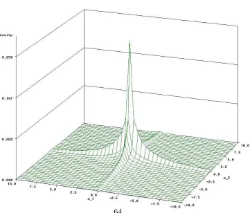
The joint density function, which is depicted in Figure 4b, can be shown as
(12)(1 2) =Π 2
=1 µ
3
2exp ()Φ
µ −3 √ 2 ¶
− 12Φ
µ − √ 2 ¶¶ (38) For cases where some of the 0, we can replace those items in the
above expression by () = 1−(−)and() =(−).
Corollary 2 In general, if we have threshold variables,
−1−2(0)
2
0 (b−0)◦
(0
1 0)
→ arg max
(1)∈
X
=1 µ
−1
2||+()
¶
(39) where ◦ is the Hadamard product operator that multiplies on an element by element basis, and
(1)(1 )
=Π=1
µ
1 +
r
2exp
µ
−
8
¶
+3 exp () 2 Φ
µ−3√
2
¶
− + 5
2 Φ
µ−√
2
¶¶
(40)
(1)(1 ) =Π
=1
µ
3
2exp ()Φ
3
A Fast Estimation Algorithm for
when x
, z
1and z
2are Independent
The threshold values are obtained by grid search, which implies that the estimation time increases exponentially with the number of threshold variables. We propose a fast estimation method when the regressors and the threshold variables are all mutually independent. Consider the fol-lowing simple model with a single regressor and two threshold variables:
=1+Ψ¡0¢+ (42) Note that the asymptotic results are the same as the case where all
= 1. From Appendix A2, it can be shown that
sup (12)∈2
¯ ¯ ¯ ¯ 1 ¡
12¢−(1 2)
¯ ¯ ¯
¯=(1) (43)
Let
(1 2) =2 ¡
(1 2)−2 ¢
for = 1234 (44)
When, 1 and2 are independent, the following can be shown.
Case 1: 1 ≤0
1 2 ≤02
1(1 2) =21¡01 ¢
2¡02 ¢µ
1− 1(
0
1)2(02)
1(1)2(2) ¶
(45)
1(1 2)
1 =−
21(01) 2
2(02) 2
1(1)2(2)
1(1)≤0 (46)
1(1 2)
2 =−
21(01) 2
2(02) 2
1(1)2(2)
2(2)≤0 (47)
where 1(1) and 2(2) are the hazard functions of 1 and 2 respectively.
Case 2: 1 0
1 2 ≤02
2(1 2) =22 ¡
02¢2
Ã
1(01)
2(02)
− 1(1)
2(2) −
¡
1(01)−1(1) ¢2
1−1(1)2(2) !
(48)
2(1 2)
1 =
21(01) 2
2(2) µ
1−1(01)2(2)
1−1(1)2(2) ¶2
2(1 2)
2
=−22 ¡
02¢2
µ
1(01)−1(1)
1−1(1)2(2)
+ 1
2(2) ¶
1−1(01)2(2)
1−1(1)2(2)
1(1)2(2)
0 (50)
Case 3: 1 ≤0
1 2 02
3(1 2) =21 ¡
01¢2
Ã
2(2)
1(1)
− 2( 0 2)
1(01) −
¡
2(02)−2(2) ¢2
1−1(1)2(2) !
(51)
3(1 2)
1
=−21¡01
¢2µ 2(20)−2(2)
1−1(1)2(2)
+ 1
1(1) ¶
1−2(02)1(1)
1−1(1)2(2)
2(2)1(1)
0 (52)
3(1 2)
2 =
2 1¡01
¢2µ 2(20)−2(2)
1−1(1)2(2)
− 1
1(1) ¶2
1(1)2(2)0 (53)
Case 4: 1 0
1 2 02
4(1 2) =2 ¡
1−1 ¡
01¢2 ¡
02¢¢
µ
1− 1−1( 0
1)2(02)
1−1(1)2(2) ¶
(54)
4(1 2)
1
=2
µ
1−1(01)2(02)
1−1(1)2(2) ¶2
2(2)1(1)0 (55)
4(1 2)
2 =
2 µ
1−1(01)2(02)
1−1(1)2(2) ¶2
1(1)2(2)0 (56)
Note that given 2, the value of (1 2) reduces whenever 1
ap-proaches 0
1 from both directions. Similarly, given 1, the value of
(1 2)reduces whenever 2 approaches0
2. This implies that
min
1∈
and
min
2∈
(1 2) =0
2 ∀1 (58)
Thus, if,1and2are independent, we can search for the critical
threshold value of one threshold variable by assigning an arbitrary value to another threshold estimate. This will dramatically shorten the time of estimation.
4
Model with Panel Data
In this section, we consider a model for a balanced panel with individ-uals over periods. We assume that the threshold values are the same
across individuals for each of the threshold variables. In the panel model here,is the cross-sectional sample size. The analysis is asymptotic with fixed and as → ∞
We let
Ψ() =(1 1 2 2)
The observations are divided into two regimes depending on whether the threshold variable vector satisfies the threshold conditions. We as-sume that and are not time invariant. The model is
=+01+ Ψ() = 0 (59)
=+02+ Ψ() = 1 (60)
The following assumptions are imposed:
(1)For each , ( ) are i.i.d. across .
(2) For each , is i.i.d. over , is independent of { }=1,
and () = 0;
(3) For each = 1 , Pr¡1 =2 ==¢ 1, where
is the th element of
(4)||4 ∞ and ||4 ∞; (5) =− where 6= 0 and 0 1
2;
(6) At = 0 and = 12, (1 2), and (1 2) are continuous;
(7) 0 ∞;
(8) For , |(01 02|01 02) ∞, where |(01 02|01 02) is the value of the conditional joint density of evaluated at the true
Assumptions (1)-(4) are standard for fixed effect panel models with exogenous regressors. Assumption (5)implies that the threshold effect tends to zero at a specified rate, which gives a well-defined distri-bution of the threshold estimators. Assumption (6) excludes
thresh-old effects that occur simultaneously in the marginal distribution of the regressors and in the regression function. Assumption (7) excludes
continuous threshold models (Chan and Tsay, 1998). (8)rules out the
possibility that all observations of the threshold variables equal the true threshold values.
Let
() =Ψ() (61)
=+01+0Ψ() + (62) Averaging the above panel equation over, we have
=+01+0() + (63)
where
= 1
X
=1
(64)
= 1
X
=1
(65)
() = 1
X
=1
Ψ() (66)
= 1
X
=1
(67)
Taking the difference, we have
∗ =01∗+0∗() +∗ (68)
where
∗=− (69)
∗() =()−() (71)
∗ =− (72)
Let
∗ =
⎡ ⎢ ⎣
∗2
... ∗ ⎤ ⎥ ⎦ ∗ = ⎡ ⎢ ⎣
∗2
... ∗ ⎤ ⎥ ⎦ ∗ () = ⎡ ⎢ ⎣
∗2()
... ∗() ⎤ ⎥ ⎦ ∗ = ⎡ ⎢ ⎣
∗2
...
∗ ⎤ ⎥ ⎦
denote the stacked data and errors for an individual, with one time period deleted. Let ∗, ∗() and ∗ denote the data that is stacked over all individuals, i.e.,
∗ = ⎡ ⎢ ⎢ ⎢ ⎢ ⎢ ⎣ ∗ 1 ... ∗ ... ∗ ⎤ ⎥ ⎥ ⎥ ⎥ ⎥ ⎦ ∗ = ⎡ ⎢ ⎢ ⎢ ⎢ ⎢ ⎣ ∗ 1 ... ∗ ... ∗ ⎤ ⎥ ⎥ ⎥ ⎥ ⎥ ⎦ ∗() = ⎡ ⎢ ⎢ ⎢ ⎢ ⎢ ⎣ ∗ 1()
... ∗ () ... ∗() ⎤ ⎥ ⎥ ⎥ ⎥ ⎥ ⎦ ∗ = ⎡ ⎢ ⎢ ⎢ ⎢ ⎢ ⎣ ∗ 1 ... ∗ ... ∗ ⎤ ⎥ ⎥ ⎥ ⎥ ⎥ ⎦
Thus, our model becomes
∗ =∗1+∗()δ+∗ (73) As the panel model can be rewritten in the form given in Section
(21), withcorresponding to, and as assumption set B is weaker than assumption set A, the estimation method and the asymptotic results in the previous section apply in the panel model. Thus, we have
() = ( −∗1−∗()δ)0( −∗1−∗()δ)
b
= (b1b2) = arg min
∈Γ
(1 2) (74)
Γ=Π2=1³h i∩(∪=1{1 }) ´
(75)
The final structural estimators are then defined as
b
and
b
2(b1b2)
and the residual variance is
b
2 = 1
( −1)(b) (76)
5
Inference
5.1
Testing the number of threshold variables
We start with a threshold model without thresholds, and sequentially test whether this model can be rejected in favor of a threshold model with one additional threshold variable. For the test of no threshold against one threshold variable,
0:= 0
1:= 1 Define
(011) = (−∞−∞)− (b1−∞)
(b1−∞) (77)
(012) = (−∞−∞)− (−∞b2)
(−∞b2) (78)
where
(−∞−∞)is the residual sum of squares from the regression
with-out any threshold variable;
(b1−∞)is the residual sum of squares from the regression with-out the second threshold variable; and
(−∞b2)is the residual sum of squares from the regression with-out the first threshold variable.
For the notation (···), the first entry in the parenthesis stands for the value of under the null hypothesis, the second represents the
value of under the alternative hypothesis, and the last indicates that the test is on the threshold variable.
0:= 1
1:= 2 Define
(121) = (b1−∞)− (e1e2)
(e1e2) (79)
(122) = (−∞b2)− (e1e2) (e1e2)
(80)
where (e1e2) is the residual sum of squares from the regression by imposing both threshold variables. If the null is rejected in both cases, then we conclude that there are two threshold variables. If we reject the null in thefirst step for thefirst threshold variable and cannot reject it in the second test, then the first variable is the only threshold variable. A similar argument applies to the second threshold variable. The problem arises when we reject the null in the first step but accept it in the second step for both variables, which should not occur in large samples. In a finite sample where such a situation occurs, we choose the threshold variable that best fits the model.
The asymptotic distributions of the above tests are non-standard. For the case of 0: = 0 against 1: = 1, the bootstrapping method in Hansen (1999) is conducted for each potential candidates of threshold variables. For the tests in the following steps, first we treat the regressors and the threshold variables as given, holding their values fixed in repeated bootstrap samples. We then use the regression resid-uals under 1 as the empirical distribution. A sample of size with replacement is drawn from this empirical distribution and the errors are used to create a bootstrap sample under 0 The values of structural and threshold parameters are fixed at their estimated values under0. We repeat this procedure for a large number of times and calculate the percentage of draws for which the simulated statistic exceeds the actual. This is the bootstrap estimate of the asymptotic p-value under0. The null is rejected if the p-value is too small.
For illustration, consider a panel model, we test
0:= 1
1:= 2
= 12 ). We then use the bootstrap residuals along with the
es-timated threshold model with one threshold variable to generate the bootstrap dependent variable:
∗ =b01∗+³b02−b01´∗Ψ(b1) +b∗ (81)
Using the set of dependent and independent variables ©x∗ ∗
ª
, we can estimate the model under the alternative hypothesis (in this case, a threshold model with two threshold variables) and compute its sum of squared residuals
³ e
1e2´ The sum of squared residuals under
the null is (b1−∞) =
P
=1
P
=1 ³
b∗´2 The test statistic for testing
two threshold variables under the alternative hypothesis against the null hypothesis that only the first threshold variable should appear in the model is
(121) =
(b1−∞)−³e1e2´
³ e
1e2´ (82)
For testing whether only the second threshold variable should appear in the model, the test statistic is
(122) = (−∞b2)−
³ e
1e2´
³e1e2´
(83)
5.2
Testing the threshold values
After obtaining the number of threshold variables, we proceed to test the hypothesis that
0 : =0
Under the assumption that is i.i.d. (0 2), we have
(1 2) = (1 2)− (b1b2) (b1b2)
(84)
0 is rejected for a large (01 02)
If the threshold variables are independent, one can show that
¡01 02¢→ 2 (85) where
1 = max
−∞1∞
(−|1|+ 21(1)) (87)
2 = max
−∞2∞
(−|2|+ 22(2)) (88) and
2 =
0
20 (89)
The distribution of (= 12)is
Pr ( ≤) =³1−−12 ´2
(90)
() =³1−−12 ´
−12 (91)
Thus,
Pr ( ≤) = Pr (1+2 ≤) =
Z
0
Pr (1 ≤−)2()
= 1−(+ 5)−−2 (−2)−12 (92)
The density function is given by
() = (+ 4)−+ (−4)−12 (93)
For= 3, we have
Pr (≤) = Pr (1+2+3 ≤)
=
Z
0
Pr (1+2 ≤−)3()
=1 2
−2³62+ 14+ 22+2−643
2+ 16 3
2−22 3 2
´
and
() = 1 2
−2³483
2−12−2−48−12 3
2+2 3 2
´
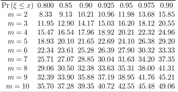
Pr (≤) 0800 085 090 0925 095 0975 099
= 2 833 913 1021 1096 1198 1368 1585
= 3 1195 1290 1417 1503 1620 1812 2055
= 4 1547 1654 1796 1892 2021 2232 2496
= 5 1893 2010 2165 2269 2410 2638 2920
= 6 2234 2361 2528 2639 2790 3032 3333
= 7 2571 2707 2885 3004 3163 3420 3735
= 8 2906 3050 3238 3363 3531 3800 4131
= 9 3239 3390 3588 3719 3895 4176 4521
[image:22.595.151.439.126.274.2]= 10 3570 3728 3935 4072 4255 4548 4906
Table A: Asymptotic Critical Values
In general, if there are threshold variables, we can derive the
dis-tribution function of uniquely from the moment generating function
() =
µ
1
(1−) (1−2)
¶
for 05 (94)
For the estimation of the nuisance 2, we can extend the results of Hansen (2000). In our case for = 2, it can be estimated via a
poly-nomial regression with (1 12 2 22 12) as the set of regressors, or via the the Nadaraya-Watson kernel estimator with a bivariate Epanech-nikov kernel.
6
Simulations
In all of the experiments below, we set = 1for all, so that the model
becomes
=1+Ψ() +
We simulate the case whereΨ() =Π2=1 ¡
¢
is set to be (01) 0
1 = 0, 02 = 0 1 = 1 = 1000 (sample size); = 10000 (number of replications); ∼ .(01),
= 1, = 1
8. All of the simulations are done in GAUSS. The codes are
available from the authors upon request.
Experiment A. This experiment simulate the behavior of the
resid-ual sum of squares and the distribution of b1(b) and b2(b) for a fixed break with 1 = 1 2 = 2. We estimate the following model:
Figure 1a plots the 3D graph of 1
¡
12¢
[image:23.595.115.492.350.635.2]Figure 1b plots the 3D graph of¡12¢
FIGURES 1a and 1b HERE
Figure 2a plots the distribution of12³b 1
¡ b
1b2¢−1´
Figure 2b plots the distribution of12³b 2
¡ b
1b2¢−2´
Figure 2c plots the 3D distribution of12³b 1
¡ b
1b2¢−1b2¡b1b2¢−2´
FIGURES 2a−2c HERE
Experiment B. This experiment studies the distribution ofb for a shrinking break. Let =2−1 =−18.
In this case, we have
(b1b2) = arg min
(12)∈Γ
¡12¢= arg min
(12)∈Γ
£
¡12¢− ¡0102¢¤
From Appendix A3, for1 =0 1+
1
1−2,2 =
0 2+
2
1−2,[1 2]∈ 2, we have
¡12 ¢
− ¡0102 ¢
=−01 ⎛
⎝1+ 2−
|1|2 X
=1
⎞ ⎠−02
⎛
⎝2+ 2−
|2|2 X
=1
⎞ ⎠
where
and are independent. Let
1 =− 0 11
2 =− 0 22 When1 and 2 are independent, we have:
1−2¡1 ¡
01¢2 ¡
02¢ ¡b1−01 ¢
2 ¡
02¢1 ¡
01¢ ¡b2−02 ¢¢
→ arg max
(12)∈2 2 X
=1 µ
−1
2||+()
¶
1 ¡
01¢=2 ¡
02¢=1(0) =
1
√
2
1 ¡
01¢=2 ¡
02¢=1(0) =
1 2
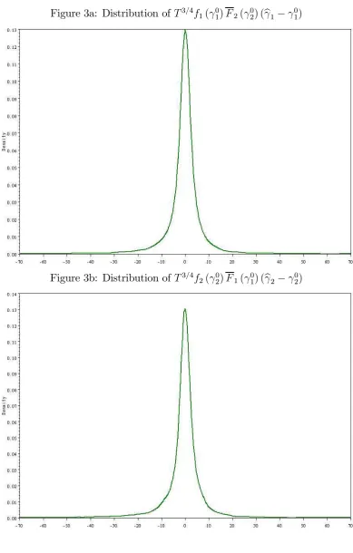
Figure 3a plots the distribution of34
1(01)2(20) (b1 −01)when
2−1 =−18
Figure 3b plots the distribution of34
2(02)1(10) (b2−02)when
2−1 =−18
FIGURES 3a and 3b HERE
Figure 4a plots the 3D distribution of
1−2¡1¡01 ¢
2¡02 ¢ ¡
b
1−01¢ 2¡02 ¢
1¡01 ¢ ¡
b
2−02¢¢
when 2−1 =−18
Figure 4b plots the joint density (12)(1 2) the definition of
which is provided in eqt.(38).
FIGURES 4a and 4b HERE
Experiment C. This experiment studies the distribution of the LR
test and plot the confidence interval around the estimated thresholds for shrinking break with =2−1 =−18.
Figure 5a plots the finite sample distribution of the LR statistics
¡01 02¢= (
0
1 02)−(b1b2)
(b1b2) (95)
FIGURE 5a HERE
With = 1, = 1000, and using the 95% critical value obtained from Table 1 for = 2, Figure 5b plots the simulated 95% confi -dence interval for (1 2) around the estimated thresholds such that
(1 2) = 1198
7
Empirical Application
The empirical relevance of our findings is studied through an applica-tion to the currency crisis models. The threshold model is particularly appropriate for the currency crisis issue as all the relevant models in the literature suggest that there are significant threshold effects in the crisis indicators. Identifying critical thresholds in the crisis indicators has important policy implications as the thresholds provide guidelines for policy makers, allowing them to formulate regulatory policies to min-imize the stampede of currency crises.
Much of the empirical work on currency crises is concerned with finding relevant crisis indicators (Kaminsky, Lizondo and Reinhart, 1997; Kaminsky, 1998; Hali, 2000). While it is helpful to understand the relevance of different crisis indicators, it is equally important for policy makers to know the critical thresholds of the indicators, above which the economy is unable to sustain a stable exchange rate amidst high pressure in the foreign exchange market. Based on the theory developed in this paper, we can estimate the joint threshold values of several crisis indicators simultaneously. We apply our model to the study of currency crises in 16 countries. It is specified as follows:
=+01+ (02−01)Ψ(zγ) + (96)
for= 1216, where
Ψ¡z 0¢=Π=1¡z 0
¢
(97)
for = 12
A currency crisis will not be triggered until all of the threshold vari-ables exceed the critical thresholds. The number of threshold varivari-ables
() to be included in the model is determined by the tests that have
been discussed in Section 5.1. The fixed effect transformation described in Section 4 is used to remove the individual-specific means from the panel data.
7.1
Exchange market pressure index as the
depen-dent variable
In the threshold model, the dependent variable is taken to be the
Frankel and Rose (1996), Sachs, Tornell and Velasco (1996), and Gold-stein, Kaminsky and Reinhart (2000). The exchange market pressure index is defined as:
≡[(1 %∆) + (2 ∆(− ))−(3 %∆)] (98) where
%∆denotes the percentage change in the exchange rate of country
i with respect to the U.S. dollar at time;
∆(− )denotes the change in the differential between the short-term discount rate in country and the US at time;
%∆denotes the percentage change in the foreign exchange reserves
of country at time ; and
1 2 and 3 are the weights that are defined as the inverse of the standard deviations of the respective components over the past ten years. The weights are assigned in order to equalize the volatilities of these three components.
7.2
Choice of the threshold variables
and
regres-sors
The threshold variables should be exogenous indicators of currency
external illiquidity is a crucial threshold variable in financial and cur-rency crises (McKinnon and Huw, 1996; Chang and Velasco, 1998a and 1998b). Given the implications of these theories, an important empirical question should be whether there are threshold effects in the threshold variables and, if so, what the threshold values are.
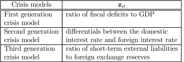
Table 1 summarizes the threshold variables for the three
gen-erations of currency crisis models. The ratio of fiscal deficit to GDP is measured as the total government expenditure minus the total gov-ernment revenue, normalized by GDP. The interest rate differential is constructed as the difference between the 3-month domestic and the US lending rates. Short-term external liabilities are measured as the sum of the short-term external debt, the cumulative portfolio liabilities and six-month imports. When the values of these threshold variables are too high, the economy enters into an unstable state and the risk of currency depreciation is imminent.
We include two fundamentals as the explanatory variables () in
the threshold regression model. These variables include the real ex-change rate and the ratio of domestic credit to GDP (Edwards, 1989; Dornbusch, Goldgajn and Valdˇs, 1995; Frankel and Rose, 1996; Sachs, Tornell and Velasco, 1996), both in natural log. The real exchange rate index measures the change in the real exchange rate relative to the base period (1986 Q1) and is employed to capture the degree of exchange rate misalignment over the sample period. In the literature, it is presumed that a large cumulative appreciation in the real exchange rate index sig-nifies a high possibility that the real exchange rate is overvalued; hence, there is a stronger pressure for the real exchange rate to revert to the mean. This measure of misalignment is only an indirect measure and does not control for long-run productivity changes; nevertheless, it re-mains common in the literature because it helps to identify countries that have experienced extreme overvaluations.
Crisis models z
First generation ratio of fiscal deficits to GDP crisis model
[image:28.595.139.452.125.231.2]Second generation differentials between the domestic crisis model interest rate and foreign interest rate Third generation ratio of short-term external liabilities crisis model to foreign exchange reserves
Table 1: Threshold variables implied by the three generations of currency crisis models
7.3
Testing the number of threshold variables
In this section, we apply the tests described in Section 5.1 to test for the presence of threshold effects. The asymptotic distribution of the test sta-tistic is non-standard and generally depends on the moments of the sam-ple. We conduct a bootstrap procedure as follows: First, we estimate the model under the alternative hypothesis. Then, we group the regression residuals (after fixed-effect transformation) b∗ by individual b∗ =(b∗
b∗2..., b∗) and draw, with replacement, error sample of individual i
b∗ ( = 12 ) from this empirical distribution b∗ This gives the bootstrap errors. The bootstrap dependent variable∗
is then generated
based on the estimatesbandb of the threshold model under the null
hy-pothesis. From the bootstrap sample©∗
∗
ª
, the test statistic is calcu-lated. This procedure is repeated a large number of times and the p-value of the test statistic is calculated as = 1 P=1© ª where is the test statistic computed from one bootstrap sample, is
the test statistic computed from the actual data, and B is the number of bootstrap replications. In this paper, 300 bootstrap replications are used for each of the tests. The null hypothesis is rejected if the p-value is smaller than the desired significance level.
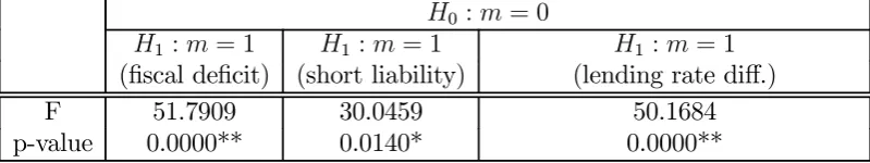
The test statistics and p-values for testing zero against one, one against two, and two against three threshold variables are performed. The results are reported in Tables 2(a), 2(b) and 2(c). The tests for zero against one threshold variable are all highly significant, with p-values of 0.000, 0.014 and 0.000 when the threshold variable is fiscal deficits, short-term external liabilities and the lending rate differentials, respec-tively.
fis-0 : = 0
1 := 1 1 := 1 1 := 1 (fiscal deficit) (short liability) (lending rate diff.)
F 51.7909 30.0459 50.1684
p-value 0.0000** 0.0140* 0.0000**
Note: The numbers in parentheses are the p-values. “**” means the test statistic is significant at the 5% level and “*” means the test statistic is significant at the 1% level. 300 bootstrap replications are used for each of the test.
Table 2: (a) Testing one threshold variable against no threshold variable
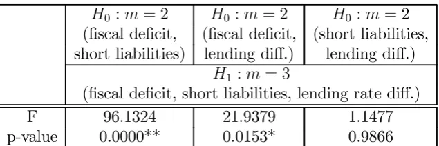
cal deficit and short-term external liabilities, and from the pair of fiscal deficit and the lending rate differential under the alternative hypothe-sis. The p-values for these two cases are 0.9667 and 1. When testing two against three threshold variables, the null hypothesis that the fiscal deficit variable can be dropped from the list of three is not rejected and the p-value is 0.9866. Based on these results, we conclude that there is strong evidence for two threshold variables in the regression relation-ship, namely, the ratio of short-term external liabilities to reserves and the lending rate differential. For the remainder of the paper we work with a threshold model with these two threshold variables.
[image:29.595.111.511.127.202.2]0 := 1 0 : = 1 (fiscal deficit) (short liabilities)
1 : = 2
(fiscal deficit, short liabilities)
F 27.1031 5.3490
p-value 0.0000** 0.9667
0 := 1 0 : = 1 (fiscal deficit) (lending rate diff.)
1 : = 2
(fiscal deficit, lending rate diff.)
F 62.0889 0.3865
p-value 0.0000** 1.0000
0 := 1 0 : = 1 (short liabilities) (lending rate diff.)
1 : = 2
(short liabilities, lending rate diff.)
F 91.0530 22.8329
p-value 0.0000** 0.0000**
Table 2: (b) Testing two threshold variables against one threshold vari-able
0 : = 2 0 := 2 0 : = 2 (fiscal deficit, (fiscal deficit, (short liabilities, short liabilities) lending diff.) lending diff.)
1 : = 3
(fiscal deficit, short liabilities, lending rate diff.)
F 96.1324 21.9379 1.1477
p-value 0.0000** 0.0153* 0.9866
[image:30.595.168.421.163.434.2] [image:30.595.136.454.557.663.2]7.4
Estimation Results
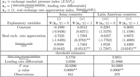
In this section, we estimate the threshold values for the ratio of short-term external liabilities to reserves and the lending rate differential. To allow for different thresholds for countries in different geographical re-gions, we divide the sample countries into the Asian and Latin American regions. The estimation results are represented in Table 3. The point estimates of the ratio of short-term external liabilities to reserves for the Asian and Latin American countries are 3.1758 and 3.9851 respec-tively. The point estimates for the lending rate differential for the Asian and Latin American countries are 2.0566 and 21.8866 percentage points (or 205.66 and 2188.66 basis points) respectively. The test statistics for
0 : = 0 against 1 : = 2 are highly significant for countries in both regions. The test statistic, along with the p-value, are 33.8296 and 0.0000 for the Asian countries and 34.0269 and 0.0000 for the Latin American countries. The p-values obtained using the bootstrap proce-dure discussed in Section 7.3 give strong evidence of threshold effects. When both threshold variables exceed their critical thresholds, the risk of currency depreciation is imminent. These threshold estimates can be used to formulate regulatory policies to reduce the risk of a currency crisis.
The coefficients of the ratio of domestic credit to GDP for both the Asian and the Latin American countries are significantly positive when both threshold variables surpass the critical thresholds (that is, when
Ψ(zγ) = 1). This indicates that the vulnerability of the banking
sector is a crucial factor in determining the exchange market pressure under this regime.
7.5
A Graphical Analysis of the Threshold E
ff
ects
We analyse how well these threshold values can be used to distinguish the normal regime from the crisis regime in foreign exchange markets. Given (1) the threshold estimates of 3.1758 for the short-term external liability variable and 2.0566 for the lending rate differential variable for Asian countries, and (2) the estimates of 3.9851 and 21.8866 for the Latin American countries, we define crisis episodes as extreme values of the exchange market pressure index,= 1 if + 3
y ≡exchange market pressure index ()
z ≡{short term external liabilitiesreserves , lending rate differentials}
x ≡{1 real exchange rate appreciation index, Domestic creditGDP }
Asian countries Latin American countries
() () () ()
Explanatory variables Ψ(zγ) = 0 Ψ(zγ) = 1 Ψ(zγ) = 0 Ψ(zγ) = 1
Constant -0.1989 0.0512 0.2281 0.3692
(-0.9436) (0.6371) (1.5579) (1.1598) Real exch. rate appreciation -2.7235 1.7293 -0.6257 3.8072
(-1.8493) (6.2783)** (-1.7762) (1.4069) Domestic credit
GDP 0.0588 1.7464 1.0528 3.4369
(0.0442) (6.0512)** (1.7287) (3.0245)** threshold estimates
Short term external liabilities
Reserves 3.1758 3.9851
Lending rate differentials 2.0566 21.8866
stat 33.8296 34.0269
p value 0.0000** 0.0000**
Observations 641 379
[image:32.595.109.579.279.539.2]Note: The numbers in parentheses are the t-statistics. “**” means that the t statistic is significant at the 5% level and “*” means that the t statistic is significant at the 1% level.
where and are, respectively, the mean and standard
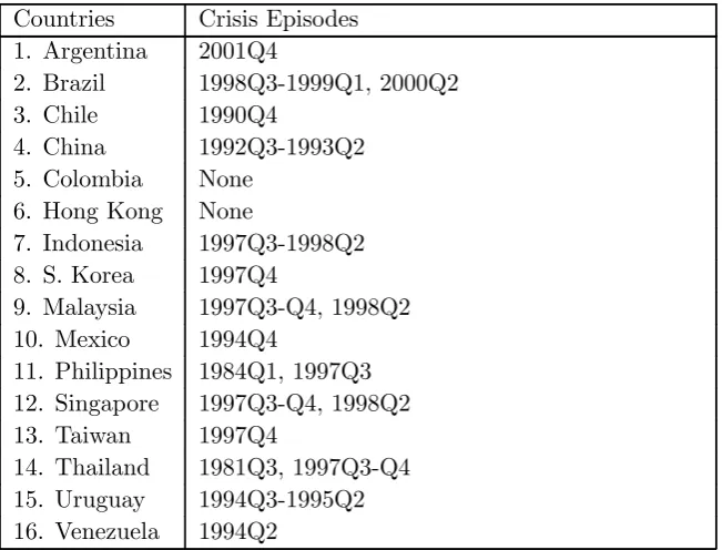
deviation of the exchange market pressure index for country i at time t. The dates of the crisis episodes in the sample are reported in Table 4.
The threshold effects are illustrated in Figures 6 and 7, which show the values of the threshold variables (represented by the bars in thefi g-ures), the critical thresholds (the dashed lines), and the exchange market pressure index (the solid lines) of the Latin American and Asian coun-tries. The crisis episodes are shaded in grey. The figures indicate that the threshold variables perform reasonably well in predicting the regime shifts. For instance, Figures 6(c) and 6(d) show that the ratio of short-term external liabilities to reserves and the lending rate differentials in Indonesia and South Korea started to exceed the critical thresholds less than two years before the 1997 financial crisis, and remained above the thresholds at the outbreak of the crisis. Figure 6(f) indicates that the 1997 currency crisis in the Philippines occurred as soon as the short-term external liabilities exceeded the critical threshold, given that the lending rate differential had already surpassed the threshold prior to the crisis. Figure 7(b) indicates that both the ratio of short-term external liabilities to reserves and the lending rate differential started to go above the critical thresholds less than one year prior to the Brazilian crisis of 2000, and remained above the thresholds throughout the crisis. Figure 7(g) shows that the 1994 Venezuelan crisis broke out as soon as the short-term external liabilities moved above the critical threshold, given that the lending rate differential had, at that time, already gone above the critical threshold.
Countries Crisis Episodes 1. Argentina 2001Q4
2. Brazil 1998Q3-1999Q1, 2000Q2
3. Chile 1990Q4
4. China 1992Q3-1993Q2
5. Colombia None 6. Hong Kong None
7. Indonesia 1997Q3-1998Q2 8. S. Korea 1997Q4
9. Malaysia 1997Q3-Q4, 1998Q2
10. Mexico 1994Q4
11. Philippines 1984Q1, 1997Q3 12. Singapore 1997Q3-Q4, 1998Q2
13. Taiwan 1997Q4
14. Thailand 1981Q3, 1997Q3-Q4 15. Uruguay 1994Q3-1995Q2 16. Venezuela 1994Q2
[image:34.595.126.452.124.372.2]Note: Crisis episodes that occurred within one year of each other in the same country are considered as one continuous episode.
Table 4: Dates of Crisis Episodes
8
Conclusion
variable in currency crises. We find overwhelming evidence of threshold effects in the ratio of short-term external liabilities to reserves and in the lending rate differential. Our finding provides strong empirical support for the currency crisis models in the literature. More importantly, our estimates of the joint threshold values can be adopted as policy guide-lines in the regulation of short-term external borrowing and interest rate differentials. Pre-emptive measures might be taken to prevent these vari-ables from crossing the critical threshold values, in order to prevent a currency crisis from happening. Finally, it should be mentioned that the applicability of our new model extends beyond the scope of economics. It can also serve as a foundation for further studies.
References
1. Astatkie, T., D. G. Watts, and W. E. Watt (1997). Nested Thresh-old Autoregressive (NeTAR) Models. International Journal of Forecasting 13, 105-116.
2. Bai, J. (1997). Estimating Multiple Breaks one at a time. Econo-metric Theory 13, 315-52.
3. Bai, J. and P. Perron (1998). Estimating and Testing Linear Mod-els with Multiple Structural Changes. Econometrica 66(1), 47-78.
4. Bautista, C. (2000). Boom-bust Cycles and Crisis Periods in the Philippines, a Regime-switching Analysis. Working paper, the University of the Philippines.
5. Bhattacharya, P. K, and P. J. Brockwell (1976). The Minimum of an Additive Process with Applications to Signal Estimation and Storage Theory. Z. Wahrschein. Verw. Gebiete, 37, 51-75.
6. Billingsley, P. (1968). Convergence of Probability Measures. New York: John Wiley and Sons.
7. Calvo, G. and G. Mendoza (2000). Capital Markets Crises and Economic Collapse in Emerging Markets: An Informational-Frictions Approach. American Economic Review Papers and Proceedings 90(2), 59-64.
9. Chan, K. S. and R. S. Tsay (1998). Limiting Properties of the Least Squares Estimator of a Continuous Threshold Autoregressive Model. Biometrika 85, 413-426.
10. Chang, R. and A. Velasco (1998a). Financial Fragility and the Exchange Rate Regime, NBER WP6469.
11. Chang, R. and A. Velasco (1998b). Financial Crises in Emerging Markets: A Canonical Model, Federal Reserve Bank of Atlanta, working paper.
12. Chen, H., T. T. L. Chong and J. Bai (2012). Theory and Applica-tions of TAR Model with two Threshold Variables. Econometric Reviews 31(2), 142—170.
13. Chen, R. and S. Tsay (1993). Functional-coefficient Autoregressive Models. Journal of the American Statistical Association 88, 298-308.
14. Chong, T. T. L. (2001). Structural Change in AR(1) Models. Econometric Theory 17, 87-155.
15. Christiano, L. J. (1992). Searching for a Break in GNP. Journal of Business & Economic Statistics 10, 237-250.
16. Dornbusch, R., I. Goldgajn and R. O. Valdˇs (1999). Currency
Crises and Collapses. Brookings Papers on Economic Activity, No.2, 219-95.
17. Durlauf, S. N. and P. A. Johnson (1995). Multiple Regimes and Cross-country Growth Behavior. Journal of Applied Econometrics 10, 365-384.
18. Edison, H. J. (2000). Do Indicators of Financial Crises Work? An Evaluation of an Early Warning System. Board of Governors of Federal Reserve System, International Finance Discussion Papers Number 675.
19. Edwards, S. (1989). Real Exchange Rates, Devaluations, and Ad-justment: Exchange Rate Policy in Developing Countries, Cam-bridge, Massachusetts: MIT Press.
21. Eichengreen, B., Rose, A., and C. Wyplosz (1996). Contagious Currency Crises, NBER WP5681.
22. Flood, R. and P. Garber (1984). Collapsing Exchange Rate Regimes: Some Linear Examples. Journal of International Economics 17,
1-13.
23. Frankel, J. A. and A. Rose (1996). Currency Crashes in Emerging Markets: Empirical Indicators,NBER WP5437.
24. Garcia, R. and P. Perron (1994). An Analysis of the Real Interest rate under Regime Shifts. Review of Economics and Statistics 78, 111-125.
25. Goldstein, M., G. Kaminsky and C. Reinhart (2000). Assessing Financial Vulnerability — An Early Warning System for Emerging Markets, Institute for International Economics 51, 145-168.
26. Gonzalo, J. and J. Pitarakis (2002). Estimation and Model Se-lection Based Inference in Single and Multiple Threshold Models.
Journal of Econometrics 110, 319-352.
27. Hali, J. E. (2000). Do Indicators of Financial Crises Work? An evaluation of the early warning system. Board of Governors of Federal Reserve System, International Finance Discussion Paper #675.
28. Hansen, B. E. (1999). Threshold Effect in Non-dynamic Panels: Estimation, Testing, and Inference. Journal of Econometrics 93,
345-368.
29. Hansen, B. E. (2000). Sample Splitting and Threshold Estimation.
Econometrica 68, 575-603.
30. Henry, Ó., N. Olekaln and P. M. Summers (2001). Exchange Rate Instability: a Threshold Autoregressive Approach. Economic Record 77, 160-166.
31. Kaminsky, G. L. (1998). Currency and Banking Crises: The Early Warnings of Distress. Board of Governors of the Federal Reserve System, International Finance Discussion Papers Number 629.