Bi Criteria Optimization Technique in Stochastic System Maintenance Allocation Problem

Bi-Criteria Optimization Technique in Stochastic System

Maintenance Allocation Problem

Irfan Ali*, S. Suhaib Hasan

Department of Statistics & Operations Research, Aligarh Muslim University, Aligarh, India Email: *[email protected]

Received November 11, 2012; revised December 15, 2012; accepted December 28,2012

ABSTRACT

In this paper, the problem of optimum allocation of repairable and replaceable components in a system is formulated as a Bi-objective stochastic non linear programming problem. The system maintenance time and cost are random variable and has gamma and normal distribution respectively. A Bi-criteria optimization technique, weighted Tchebycheff is used to obtain the optimum allocation for a system. A numerical example is also presented to illustrate the computa-tional details.

Keywords: Selective Maintenance; Weighted Tchebycheff Technique; Multi-Criteria Optimization; Stochastic Programming; Chance Constrained; Modified E-Model; System Reliability

1. Introduction

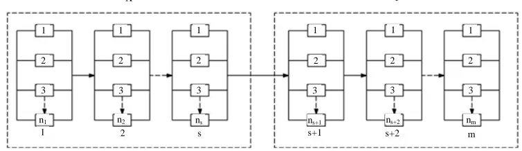
We consider a system which requires performing a se-quence of identical production runs after every given (fixed) period. A production run in the system consists of several subsystems where each subsystem can work pro- perly if at least one of its components is operational. The following assumptions are also made:

1) all the components can be repaired if deteriorated or failed;

2) all component states are independent.

We assume that the system comprises two types of subsystem. One is the type of subsystems in which the components are very sensitive to the functioning of the whole system and, therefore, on deterioration these should be replaced by new ones. Let these subsystems range from 1 to

paired and then replaced. Let such subsystems range from

s. The other type of subsystems is those in which the components after deterioration can be re-

1

s to . In Figure 1 the Group X consists of the

m

s subsystems with sensitive components which on failure are replaced by new ones and Y the remaining



ms



subsystems in which the components can be repaired (see Ali et al. [1]).

Ideally, all the failed components in all the subsystem of Group X are replaced by new ones prior to the begin-ning of the next mission/ run. In a similar way, ideally all the failed components in subsystem of Group Y are re-paired and then replaced prior to the beginning of the next mission/run. However, due to the constraints on the cost and time it may not be possible to repair and replace all the failed components in Groups X and Y. For this a mathematical programming frame-work is established for assisting decision-makers in determining the optimal subset of maintenance activities to perform prior to begin-ning of the next mission. This decision-making process

1 1 1 1 1 1

1

2 2 2 2 2 2

3 3

3 3

3 3

s m

2 s+1 s+2

n1 n2 ns ns+1 ns+2 nm

[image:1.595.109.486.598.707.2]

X Y

Figure 1. Parallel components in repairable and replaceable subsystem.

*

a d

, 1, 2, ,

i i i

n k d i  m



1

i i i

n a d i i

r  



 _{  }

 _ 

 

1

is referred to as selective maintenance. The selective maintenance models presented allow the decision-maker to consider limitations on maintenance time and budget, as well as the reliability of the system. Selective mainte-nance is an open research area that is consistent with the modern industrial objective of performing more intelli-gent and efficient maintenance.

For this let us suppose i be the total failed

compo-nents in the subsystems and i be the number of

com-ponents in the subsystem, which can be repaired and replaced prior to the beginning of the next mission (See Rice et al. [2]). Thus under the selective maintenance the number of components available for the next mission in the subsystem will be

th

i

th

i





(1) Therefore the reliability of the subsystems range from 1 to

s

for a production run is given by

 

1



1

s i

R d 



 _ (2) and the reliability of the subsystems range from s



1

i i i

n a d i i S

r  

 

 _{  }

 _{ }

 

0 1

m i i i

t d T







0 1

m

i i i

c d C







tom for a production run is given by

 

1



1

m i

R d 



 (3)

The maintenance time constraint for the system is given as

(4)

and the maintenance cost constraint for the system is given as

(5)

However, in the event the reliability of the subsystems of Groups X and Y time are of equally serious concern. Let us consider, for instance, the following multi-objective problem (please see the Equation (6) below).

Secondly, a Bi-objective programming problem in which time and the cost spent on system maintenance is minimized simultaneously for the required reliability

 

i i (say). The mathematical model of the problem

is given as Equation (7) below.

R d

 





 

 





 

 

 

 

 

1

1 0 1 0 1

Maximize 1 1 i

and Maximize 1 1 ii

Subject to iii

iv

0 , are int eger v

, 1, 2, , vi

i i i

i i i

s

n a d

i i

i m

n a d

i i

i S m

i i i m

i i i

i i i i i

R d r

R d r

t d T

c d C

d a d

n a i m

  

   







 _{ }

    

Recently many authors have discussed the allocation problem of repairable components. Among them are Rice et al. [2], Schneider and Cassady [3], Rajaopalan and Cassady [4], Schneider et al. [5], Iyoob et al. [6], Ali et al. ([1,7-10]), Faisal and Ali [11] and many others.

In this paper, we have formulated stochastic system maintenance problem as a multi-objective programming



 

  _



 _{ }

 _{ }   _{ }

  



 

 

 _

    



  _











 

 





 

 





 

 

 

 

1

0 1

1 1

2 1

Minimize i

and Minimize ii

Subject to 1 1 iii

1 1 iv

0 , are int eger v

, 1, 2, , vi

i i i

i i i

m i i i

m

i i i s

n a d

i i

i m

n a d

i i

i S

i i i

i i

T t d

C c d C

r R d

r R d

d a d

n a i m





  _



  

 

 

(6)

  

 _



 _{   }_{ }

 _{ } _

  _

 _{ } 

  

 _{ } _

  _



  



  _











(7)

problem. We have discussed components repairable and

ii)

e above pro i

i ib

ra

i



 

0



0,

P f d T  p (9) Since number of components within the

as

 

replaceable time and cost as a random variable in the constraint and has Gamma and Normal distribution re-spectively. The Probabilistic constraints function is then converted into an equivalent deterministic non-linear programming form by using chance constrained pro-gramming.

2. The Chance Constrained Programming

In many practical situations the constraint Equations (i and (iv) are not fixed and taken as probabilistic. Thus the above problem (6) can be written in the following chance constrained programming form as Equation (8) below, wherep0, 0 p01 is a specified probability.

In th blem (8), let us assume that t and

c are independently gamma and normally distr uted ndom variables.

Let us assume that t i, 1,,m

m variables

are independent Gamma distributed rando in the constraint 8 (iii), i.e., t_i ~G



 _i, _i



.

Then the,

 

Mean i

i i

t 



 , Variance

 

₂i i

i

t 

  .

 

1

m i i i Now let

f d t d







 

Then mean is

 





1 1

m m

i i i i

i i i

t  d



 









distributed we have

E f d d E

Further, as tiare independently ,

 





m 2

 

m i

V f d 



t V d 



 d

2

1 1

i i i

i i i

written as Now the constraints 8 (iii) can be

system are sumed to be large we have from Liapounoff’s central limit theorem

 

~







,



 





f d N E f d V f d .

Thus (9) is equivalent to

 





 



 





 



 





0

0,

T E f d

P p

V f d V f d

 

 _ _

 

 

 

where

 



 



 





f d E f d

 _

_{f d E f d}

V f d

 

 

 

 

is a standard normal variate

with mean zero and variance one. Thus the probability of realizing



f d

 



less than or equal to T0 can be writ-ten as

 







 



 





0

0 ,

T E f d

P f d T

V f d

  

 

 

 

(10)

where 

 

z represents the cumulative density function of the standard normal variable evaluated at Z. If K_

represents the value of the standard normal variable at which 

 

K p0, then the constraint (10) can be

writ-ten as

 





 





 

0

.

T E f d

K

V f d 

   

 

 

(11)

The inequality will be satisfied only if

 





 





0

,

T E f d

K

V f d 

 _ 

 _{ }

 

 

 





 

 





 

 

 

 

 

1

1

0 0

1

0 0

Maximize 1 1 i

and Maximize 1 1 ii

Subject to iii

iv

, are int eger v

, 1, 2, , vi

i i i

i i i

s

n a d

i i

i m

n a d

i i

i S m

i i i i i i i i i i

R d r

R d r

P t d T p

P c d C p

d a d

n a i m

  

   





 _{ }

 _   _ 

  _



 _{ }

 _   _ 

  



 _ _{ }

  

 

1 0

m i

   _ _



 

 

  

  _











(8)

or equivalently,

0

m

i m

1

2 2 1

,

i

i i i

i i i

T d

K d



   





Thus an equivalent deterministic constraint to the sto-chastic co









nstraint is given by

1

m i

i i

2 0 2 1

i

m i

i i i

d

K  d T





 

 

 







(12)

onsider se whenciare independently

om variables in the constraint 8 .

i

0 p0,is equivalent to

 



 



 







 





 





 





0

0,

f c E f c C E f c

P p

V f c V f c

 _{ } 

 _ _

 

 

 

(13)

Now in this case

 





 

1

m m

i

E f c d E c d

Now we c normally (iv), i.e.

the ca rand



2



distributed

~ ,

i i

c N  

The constraint P f



 

c C





1

i i i i

i













and

 





2

 

2 2

1 1

m m

i h i i

i i

V f c d V c  d

 









Therefore, the deterministic equivalent of 8 (iv) in this case is



2 2 0

1 1

m m

i i i i

i i

d K_ d C

 

 

 _{  }

 









(14) The equivalent deterministic non-linear programming pr stochastic programming problem is give

 

 





 

oblem (8) to the n by

 





 

 

 

iv v 1

0 2

1 1

0

ize 1 1 i

Maximize 1 1 ii

bject to iii

r ,

i

i i i

d

i i

i m

n a d i

m m

i i

i i

i i i i

i i

i i i

R d r

R d r

d K d T

d a

n a



 

 

 

 

 

   _   _

 

 _{ }

_   _

 

 

   

  











1

i S  



2

i 

2 2

1 1

m m

idi K idi C

 

 

 _{  }





_



Maxim

and

Su

0 i,diare int ege

i i

na s

 _

 

1, 2, , vi

i m

               

  _

(15)

3. Modified E-Model

Consider the situations in which the time taken and cost spent on maintenance are not fixed and taken as prob-

abilistic in the objective function in Equations (i) and (ii). Thus the above problem (7) can be written in the follow-ing probabilistic objective function form as:

 

   

 

ii

iii

v

i i i

n a d

i

R d

  



     

 

  

 

 

(16)

 

i _









1

1

1 1

Minimize

and Minimize

Subject to 1 1 1 1

0 , are int eger

, 1, 2, ,

i i i

m i i i

m

i i i

s m

n a d

i i

i i S

i i i

i

T p t d

C p c d

r r

d a d

i m



  

 

 

  

 

 

 _ _

 _{   } _{   }

 _{ }  _

  

  













 

vi 

   i

Using Modified E-model technique, the problem (16) is formulated as

 

 

   

 

i

ii

iii

iv

i

R d

  

 

v

              

es show the relative impor the expectation and the variance. Some authors suggest that k1 k2 1









2

1 2 2

1 1

2 2

1 2

1 1

1 1

Minimize

and Minimize

Subject to 1 1 1 1

0 , are int eger

,

i i i i i i

m m

i i

i i

i i i i

m m

i i i i

i i

s m

n a d n a d

i i

i i S

i i i i i

T k d k d

C k d k d

r r

d a d

n a i

 

 

 

 

 

    

  

 

  

 

 

 _{ }

 

 _{   } _{     }

 _{ }  _{ }

  

  















1, 2, ,m

 

(17)

wh valu

ere k1 and k2 are non-negative constants, and their tance of

  ,

].

The two others Bi-objective programming models in different prospects for the decision-makers are

Model 1:

see Rao [12

 

 

 





 

2

1 2 2

1 1

Minimize i

ii

iii

m m

i i

i i

i i i i

T k  d k  d

 

 

   _{ }









 

 

iv v

i

R d

 

       

 

(18)









2

1 2 2

0

1 1

1 1

and Maximize 1 1

Subject to

1 1 1 1

i i i

i i i i i i

m

n a d

i i

i S

m m

i i i i

i i

s m

n a d n a d

i i

i i S

R d r

d K d C

r r



 

   

 

   

  

 _{ }

 _   _

 

 _{  }

   

 _{ }  _{ }

    

 _{ }  _{ }

   











 

 

vi

 

0 , are int eger , 1, 2, ,

i i i i i

d a d

n a i m

     

 

Model 2:

 

 

 





 

2 2

1 2

1 1

Minimize i

ii

iii

m m

i i i i

i i

C k d k d

R

 

 

   _{ }

 

  





 









1

1

2 0 2

1 1

1 1

and Maximize 1 1

Subject to

1 1 1 1

i i i

i i i i i i

s

n a d

i i

i

m m

i i

i i

i i i i

s m

n a d n a d

i i

i i S

R d r

d K d T

r r



 

 

  

 

   

  

 _{ }

_{ }   _

 

 

 

   

 _{   } _{     }

 _{ }  _{ }

  











 

 

 

iv v vi

                

4.

ia Weighted Tchebycheff

Optimization Technique

Let us consider a multi-objective programming

prob-lem 0 , are int eger

, 1, 2, ,

i i i i

i i

d

d a d

n a i m



     

(19)

A Multi-Criter

 

1

   

2

 

Min , , ,

Subject to

k

f x f x f x f x

x s

 _



 _



ve k k



2



competing objective

func-

i 



that are to be minimized simulta-neously. The followi itions illustrate the concepts of efficient and weakly efficient decision vectors.

Definition: A or

assum tions

ed to ha : n

f  

ng defin n vec

decisio t xX is efficient ective programming

prob-, (Pareto optima

lem if there doe l) for m

a ulti-obj

s not exist xX xx such that

 

 

for

i i 1, 2, ,

f x f x holding for

i 

nde k

 

at least one i x

with strict inequality

.

i (xX is efficient,

 

f x is non-dominated).

Definition: A decision vector x X is ulti-obj not exi

_

weakly effi-mal) for m ective

pro-gram st a ,

cient (weakly Pareto ming problem

opti

if there does xX

xx such that f xi

 

fi

 



x for

 i1, 2,,k .

( xX is weakly efficient, f x

 

 is weakly no minated).

n- do

There are several metrics that are found in the litera-ture related to multi-objective programming problem. If

i

 is the reference point and the ideal point,

 

Min

i x Xfi x

   ,

rence p

is used as the refe oint, the general weighted



-me

p

L p is defined as

 



c 1   tri

1 Min

p k

p i i i

w f x  

 _ 







_{ }

1 Subject to

i

x X



 



 _

(21)

1, 2,,k and

1 1

k

i i

w



We assume that wi 0, i



 , where thewi’s are weighting coefficients provided by the

de

 

cision maker reflecting the relative importance. If p , problem (21) reduces to a “weighted Tcheby-cheff Technique” (see Bowman [13]).

1,2, ,

Min Max

Subject to

i i i

i k w f x

x X



   



 _

 ₍₂₂₎

If the reference point is the global optimal solution of

 

f_i x , then the absolute value signs in problem (22) can be removed (see Miettinen [14

 

]) yielding





1,2, ,

Min Max

Subject to

i i i i k w f x

x X



   _

 _

 ₍₂₃₎

Miettinen [14] also showed that if the objectives and constraints are differentiable form of problem (23) can be defined as

 









Min

Subject to wi fi x i , i x, X



 

 

   _{ } (24)

The solution of problem (24) is guaranteed weekly non-dominated for positive weights a

non-dominated solution is also guaranteed. If t

tion is unique, then it is non-dominated, however if it is no

Wierz

on (15) are to be maximizing the total reliability of replaceable com-ponents of Group X and the reliability of

ponents of Group Y. We have convert the following ma

nd at least one he solu-t unique, solu-then isolu-t mighsolu-t be weakly non-dominasolu-ted (see

bicki [15].

The two objective functions in the Equati

repairable com-ximizing problem into minimization problem using the property MaxZ Min

 

Z . Therefore the problem defined in Equation (15) is converted into a two criterion minimization problem: Min



Z Z1, 2



subject to the

constraints (see Khasawneh et al. [16]). Now the effi-cient solution is obtained by using the weighte bycheff technique

d

Tche- 





 





 

 

 



2 1

2

1

2 2

1

1 2 1 2

Minim

1

1 1

v

1, , 0

i

s

n a i i S



2

0

0

iii

iv

vi T

C

 

 

1 1 Subject to

i

m

w

w







  _

  

 _





1 i

1 i i i ii

i i

n a d i

d

r 



 



  

 _ _

 

  

2 1

m m

i i

1

i i i

 

ize

0

i i

i

i i

m m

i i i

r

d K d

w w w w

 

 

  





 _{ }



 _{ } 

  

 

 _{  }

 

 

  





i

t K_ d

 



 



 







 

 

vii

viii

           

(25)

, are int eger

, ,

i i i

i i

d a d

n a m





  

   _

i

,i 1, 2

     

 

 









 

 

 

 

0

i

ii

iii iv v

i i di T

  

 _{ }

 

1

1

2 2

1 1

2 2 0

1 1

Min 1 1

Subject to

0 , are int eger , 1, 2, ,

s

n a

i i

i

m m

i i

i i

i i i i

m m

i i i i

i i

i i i i i

R d r

t K d

d K d C

d a d

n a i m







 

 

 



 

 

    _   _{ }

  _

  



 

 

  



 _{ } 

 

  

   

   

   

(26)

and similarly

 













 









 

 

 

 

2

1

2 2 0

1 1

Min 1 1 i

iii

0 , are int eger iv

, 1, 2, , v

i i i

m

n a d

i i

i s

m m

2 0 2

1 1

Subject to i i ii

i i

i i

m m

i i i i

i i

i i i i i

R d r

d K d C

d a d

n a i m





 

 

   

 



 _{ }

      

i i

t K_ d T

 

 



 

  _



  _

 

 

  



 _{ } 

  

  _

   

   

   









(27)

In similar way, the problem Equation (17) is also a two criterion minimizat :





defined in

ion problem Min



T C,



subject to the constraints. Now the efficient solution is obtained by using the weighted Tchebycheff technique

 

 

 

 

Minimize i

ii

iii

i

R d





  

 

 









2

1 1 2 2 1

1 1

2 2

2 1 2 2

1 1

1 1

Subject to

1 1 i i i 1 1 i i i

m m

i i

i i

i i i i

m m

i i i i

i i

s m

n a d n a d

i i

i i S

w k t k d

w k d k d

r r

 

 

 

   

 

 

    

  

    

  

     

   

  

 

 _{ } 

 

 _{  }  _

 

 

 

 _{   } _{     }

 _{ }  _{ }

  













 

 

1 2 1, 1, 2 0 v

0 , are int eger vi

, 1, 2, , vii

i i i

i i

w w w w

d a d

n a i m

          

 

   _

 

  

 

  _





iv _ (28)

The values of i can be defined as the minimum individual values of the following problems:

 

 

 

 

 

i

ii iii

, 1, 2, , iv

i

i i

R d

   

 

 

 _

  



(29)









2

1 1 2 2

1 1

1 1

Min

Subject to 1 1 1 1

0 , are int eger

i i i i i i

m m

i i

i i

i i i i

s m

n a d n a d

i i

i i S

i i i

T k d k d

r r

d a d

n a i m

 



 

 

    

  

    _{ }

 

 _{   } _{     }

 _{ }  _{ }

  

    









and similarly

 

   

 

 

i

ii

iii

, 1, 2, , iv

i

i i

R d

n a i m

   

 

 

 _

 

   _

(30)

em

 



TR d2 i



subject to the constraints. Now the

ng the weighted









2 2

2 1 2

1 1

1 1

Min

Subject to 1 1 1 1

0 , are int eger

i i i i i i

m m

i i i i

i i

s m

n a d n a d

i i

i i S

i i i

C k d k d

r r

d a d

  

 

    _

  

 

  _{ }

 

 _{   } _{     }

 _{ }  _{ }

  

  









Now the probl defined in Model 1; Equation (18) is o a two criterion minimization problem:

efficient solution is obtained by usi Tchebycheff technique

als Min

 

 

 

 

 

Minimize i

ii

iii

iv

i

R d



  

  













2

1 1 2 2 1

1 1

2 2

1

1 1

Subject to

1 1

1 1 1 1

i i i

i i i i i i

m m

i i

i i

i i i i m

n a d i i S

s m

n a d n a d

i i

i i S

w k t k d

w r

r r

 



 

 



 

   

    

  

   

  

 _{  } _{ }

   

  

 

 _{ }   _{ }   _ _

 

 

 _{   } _{     }

 _{ }  _{ }

  











 

 

 

 

v

vi vii viii

                     







(31)

1

2 2 0

1 1

1 2 1, 1, 2 0 0 , are int eger

, 1, 2, ,

m m

i i i i

i i

i i i i i

d K d C

w w w w

d a d

n a i m

 

 

 _{  }

   

  

  

  _

The values of  and 2 is the minimum individual values obtained as

1

 

2

1 2 2

1 1

Minimize

m m

i i

i i

i i i i

T

k  d k  d

 

 

   _{ }









subject to the (iii) to (vi) of Equation (18)

 





2 2

1

Min 1 1 i i i

m

n a d

i i

i S

R d r

  

 

 _{ }

  _{ }   _







subject to the (iii) to (vi) of Equation (18).

In Model 2, Equation (19) is also a two criterion mini- mization problem: Min



CR d1

 

i



subject to the con-

straints. Now the efficient solution is obtained by using the weighted Tchebycheff technique

 

 

 

   













2 2

1 1 2 1

1 1

2 2

1

1 1

1 Minimize

Subject to

1 1

1 1 1 1

i i i

i i i i i i

m m

i i i i

i i

s

n a d i i

s m

n a d n a d

i i

i i S

m i

i i i

w k d k d

w r

r r

t 

   

 

 

 

  

    

  



 _{ } 

 

       

 

 

 _{ }   _{ }   _ _

 

 

 _{   } _{     }

 _{ }  _{ }

  

      













i

ii

iii

iv

i

R d

  

 

 

 

 

v

vi vii viii

i i

         

  

 _

    

 

   _



  _





w

2 0 2 1 1 2 1, 1, 2 0 0 , are int eger

, 1, 2, ,

m i

i i i

i i i

K d T

w w w w

d a d

n a i m



 





 (32)

here the values of 1 and 2 is the minimum indi-vidual values obtained as

2 2 2

1 1

m m

i i

i i

k  d

 







subject to the (iii) to (vi) of Equation (19)

i i di 

1 MinimizeC k1 idi

  _{ }  _

 

 





2 Min 1 1 1

s

n a

i i

R d r

 

1

i

 _

   _   _

 

subject to the (iii) to (vi) of Equation (19).

5. Numerical Illustrations

Consider a system having the Group X consisting of 3 subsystems and also the Group Y consisting of 4 subsys-tems. The available time between two missions for re-pairing and replacing is 150 time units. The available

cost of maintenance for repairing and replacing f next mission is 860 units. For simplicity we have con-sidered in the above numerical illustration: the reliability

e, cost spent p

5.1. Solution of Chance Constrained Programming by Using Weighted Tchebycheff Technique

Before applying the Weighted Tchebycheff Technique firstly we find the individual optimum values



or the

of each component in a subsystem is sam

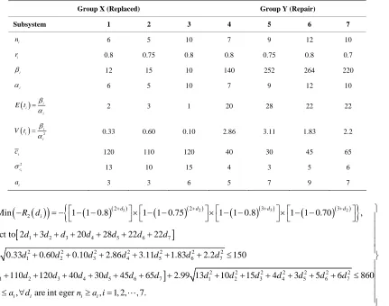
and time taken on replacing and re airing each compo-nent within a subsystem are same. The remaining pa-rameters for the various subsystems are given in Table 1.



1, 2



i

    . For the values given in Table 1, the SNLPP (26) for the first optimum value is

 











 

_

_

 

_

_

 







1 2 3

3 2 4

1 1

1 2 3 4 5 6 7

2 2 2 2 2 2 2

1 2 3 4 5 6 7

1 2 3 4 5 6

Min 1 1 0.8 1 1 0.75 1 1 0.8 ,

Subject to 2 3 20 28 22 22

2.99 0.33 0.60 0.10 2.86 3.11 1.83 2.2 150

120 110 120 40 30 45 65

d d d

i

R d

d d d d d d d

d d d d d d d

d d d d d d d

 _  _{ }  _{ }  _

    _   _{ }   _{ }   _

     

       

     



7



2 2 2 2 2 2 2

1 2 3 4 5 6 7

2.99 13 10 15 4 3 5 6 860

, 7.

d d d d d d d

        

        _



(33)

(33) provided by LINGO is

1 2, 2 3, 3 2, 6 0, 7

d  d  d  d d  d 

with the value of objective function as

0diai,diare int egernia ii, 1, 2, The optimal solution of





 

1 ij 0.9986398.

R d 

nd

4 0,d5 0,

 _{ 0}

[image:10.595.90.521.102.442.2]

iled components and the resp

Table 1. The number of fa ective cost and time etc. in the various subsystems.

Group Y (Repair) Group X (Replaced)

Subsystem 1 2 3 4 5 6 7

i

n 6 5 10 7 9 12 10

i

r 0.8 0.75 0.8

i

0.8 0.75 0.8 0.7

 12 15 10 140 252 264 220

i

 6 5 10

 

7 9 12 10

i i

i

E t _ 2 3 1 22

 

20 28 22

2

i i

i

V t 



 0.33 0.60 0.10 2.86 3.11 1.83 2.2

i

c 120 110 120

2 i

c

40 30 45 65

 13 10 15 4 3 5 6

ai 3 3 6 5 7 9 7

 











 

_

_

 

_

_

 

_

_





 



1 2

2 2 3

2 2

1 2 3 4 5 6 7

2 2 2 2 2 2 2

1 2 3 4 5 6 7

1 2 3

Min 1 1 0.8 1 1 0.75 1 1 0.8 1 1 0.70

Subject to 2 3 20 28 22 22

2.99 0.33 0.60 0.10 2.86 3.11 1.83 2.2 150 120 110 120 4

d d d

i

R d

d d d d d d d

d d d d d d d

d d d

 _  _{ }  _{ }  _{ }

    _   _{ }   _  _{ }  _

     

       

  





3 3 2

,

d  _



2 2 2 2 2

4 5 6 7 1 2 3 4 5

0 30 45 65 2.99 13 10 15 4 3 5

0 i i, iare int eger i i, 1, 2, , 7.

d d d d d d d d d

d a d n a i

2 2

6 6 7 860

d d

        

          

 

    





(34)

The optimal solution of (34) provided by LINGO is

6 1,d7 2

_  _

with the

0



(33) and (34) t optimu ues

1 0, 2 0, 3 0, 4 2, 5 1,

d  d  d d  d d

value of objective function as

 

2 ij

R d .9788431 .

From the Equations he m val



0.9986398, 0.9788431



   . For simplicity we as- su ed that th



e reliability of both the Groups X and Y 20.5. For the values gi , the SNLPP (25) effi-cient solution is ob the weighted Tche-bycheff Technique





 

_

_



















 

_

_

 

_

_

 

_

_

 

















3

4 5 6 7

3 2 4

1

2 2 3 3

2 Minimize

Subject to 1 1 .75 1 0.99 42

1 0.8 1 1 0.75 1 1 0.8 1 1 0.7 0.9994604

2 3 20 28 22 22

d

d d d d

w

w

d d d d d d d









   

 



  _{  }    _{ } 

     

 

  _  _{ }   _{ }     _{ }  

     

m

subsystems are equally important, that is w1w ven in Table 1

tained by using





  1 0.8

 _{ } d1  d2   _ 

1 2 3 4 5 6 7

2.99 0.1



1 0 1 0.8 838

1 _





2 2 2 2 2 2

0 2

1 2 3 4 5 6 7

2 2 2 2 2

1 2 3 4 5 6 7 1 2 3 4 5 6 7

1 2 1 2

5 0.18 0.10 0 0.5 0.60 150

120 110 120 40 30 45 2. 0 15 5 9 860

0 i i, iare int eger, , , , i i, 1, 2, , 7

d d d d d d d

d d d d d d d d d d

d a w w w w n a i



2

7 d2 0.35 .40

65d 99 1 8 8

1 0 .

d d

d

      

     

         

      



   

 

        

(35)

The optimum allocation under the Weighted Tcheby-cheff Technique





Tcheb 1 2 d d d d d3 4, 5, 6, 7

   

1 2, 2 3, 3 0, 4 2, 5 2, 6 0, 7 1.

d  d  d  d  d  d  d 

The corresponding value of objective function is

0.00076.

5.2. Solution of Modified E-Model by Using Weighted Tchebycheff Technique

The individual optimum values i



1, 2



, , , d  d d  

is obtained as

         . For th

lues given in Table 1 and for simplicity take k1 = k2 then the SNLPP (29) for the first optimum value is





e va- = 0.5





1 1 0.8  





 



 



2 1 2 3 4

3d 2d

  

_

_

3

1 0.8 _ 

 (36)





 

_

_

 

_

_

 

1 2

2

1 1 1 2 3 4 5 6 7

2 2 2 2 2 2 2

5 6 7

4

2

Min 2 3 20 28 22 22

0.33 0.60 0.10 2.86 3.11 1.83 2.2

Subject to 1 1 0.75 1

1 1 0.75

d d

T k d d d d d d d

k d d d d d d d







       

      

 

     

    

 

  

 

1

2 1 1 0.8 d

  





_   _ 3 3

1 1 0.8 d





  0 di ai, diare int eger,ni a ii 1, 2, , 7.

  

 

     



2

3

1 1 0.70 d 0.

 _{  }  _{ 99} 

 



 

,

 

And the SNLPP (30) for the second optimum value









 

_

_

 

_

_

 





     

1 2 3

1 2 3

2 1 1 2 3 4 5 6 7

2 2 2 2 2 2 2

2 1 2 3 4 5 6 7

3 2 4

2 2 3

MinC 120 110 120 40 30 45 65

10 8 15 8 5 7 9

Subject to 1 1 0.8 d 1 1 0.75 d 1 1 0.8 d

d d d

k d d d d d d d

k d d d d d d d



  

  

       

      

 

 _{ }  _{  } _{  }

     

 

     3













1 1 0.8 1 1 0.75 1 1 0.8 1 1 0.7





_   _{ }   _{ }   _  





 2



0 0.99

0 , are int eger, , 1, 2, , 7.

d i i i i i

d a d n a i

          _

 



      _

(37)

at is w1w20.5. For , the SNLPP (28) efficient

e weighted Tchebycheff From the Equations (36) and (37) the optimum values



101.73, 418.40



  .

For simplicity we assumed that the maintenance time

systems are equally important, th the values given in Table 1

solution is obtained by using th









taken and cost spent for both the Groups X and Y sub- Technique







5 6 7

.11 1.83 2.2 101.73

45 65

d d d

d d

  

 







0.5 120 110 120 40 30

w d d d d

      

1 1 2 3 4 5 6 7

Minimize

Subject to w 0.5 2d 3d d 20d 28d 22d 22d

2 2 2 2

1 2 3 4

2 1 2 3 4 5 6 7

2 2 2 2 2 2

3 4 5 6

0.5 0.33 0.60 0.10 2. 3

0.5 8 5 7

d d d d

d

d d d d d d

    

     

2 2 2

1 2

10 8 15

86



  













 

_

_

 









 

_

_

 

_

_

 

_

_

 





1 2 3

1 2 3 2

2 7

3 2 4

2 2 3 3

9 418.40

Subject to 1 1 0.8 1 1 0.75 1 1 0.8

1 1 0.8 1 1 0.75 1 1 0.8 1 1 0.70 0.99

0 , are int eger, , 1, 2, , 7.

d d d

d d d d

d

d a d n a i

  

   

 

    

 

 

 

        _

      _



 

     

 _   _{ }   _  _{ }  _{ }  _ 

      _

(38)

 

 

i i i i i

The optimum allocation under the Weighted Tcheby- cheff Technique

  