USING THE COMPLETE
B
AB
ARDATA SET.
Thesis by
David Andrew Doll
In Partial Fulfillment of the Requirements
for the Degree of
Doctor of Philosophy
California Institute of Technology
Pasadena, California
2011
c
Acknowledgements
I’d like to acknowledge all the folks who helped make this thesis possible: Dr. David Hitlin for his advisement; Dr. Frank Porter for answering occasionally elementary question without judgement; Piti Ongmongkolkul for the insights, the rest of the Caltech BABAR
Abstract
We present the results of a measurement of the total rate and photon energy spectrum in
b → sγ transitions using the entire BABAR data set, 429 fb−1. These results use a “sum of exclusives” approach in which we reconstruct a subset of the final states of the s-quark system and correct for the final states that are missing. We find B(B → Xsγ) = (329±
19±48)×10−6 for Eγ >1.9 GeV. We also measure the mean and variance of the photon
spectrum and find hEi = 2.346±0.018+0−0..027022 and
E2
Contents
Acknowledgements iv
Abstract v
1 Introduction 1
2 Theory 3
2.1 b→sγ Transition Rate . . . 4
2.1.1 NP Models andb→sγ . . . 8
2.2 b→sγ Photon Spectrum . . . 11
3 Analysis Procedure 14 4 PEP-II and the BABAR Detector 18 4.1 PEP-II . . . 18
4.2 The BABAR Detector . . . 20
4.2.1 Silicon Vertex Tracker . . . 23
4.2.2 Drift Chamber . . . 25
4.2.3 Detector of Internally Reflected Cherenkov Light . . . 28
4.2.4 Electromagnetic Calorimeter . . . 30
4.2.4.1 Light Yield Falloff . . . 31
4.2.5 Instrumented Flux Return . . . 32
4.2.6 Trigger . . . 34
4.2.7 Particle Identification . . . 36
5 Preliminary Event Selection 39 5.1 Event Skims and B Reconstruction . . . 39
5.2 Data Used . . . 40
6 Final Event Selection 44 6.1 π0 Veto . . . 44
6.2 Background Rejecting Classifier, BRC . . . 47
6.2.1 Variables Used in BRC . . . 48
6.2.2 BRC Final Training . . . 49
6.3 Signal-Selecting Classifier, SSC . . . 51
6.4 Final Optimized Cuts . . . 56
7 Fitting Procedure 62
7.1 Fitting Overview . . . 62
7.1.1 Signal Distribution . . . 63
7.1.2 Cross-feed Background Distribution . . . 64
7.1.3 PeakingBB Background Distribution . . . 65
7.1.4 Combinatoric Background Distribution . . . 68
7.1.5 Complete Bin Fits . . . 68
7.2 Fit Validation - Toy Studies . . . 68
8 Sideband Studies 75 8.1 Classifier Sidebands . . . 75
8.2 π0 Veto Classifier Sideband . . . . 77
8.3 High mXs Sideband, PeakingBB . . . 80
9 Fragmentation Studies 86 9.1 Different Fragmentation Models . . . 87
9.1.1 Showering Quarks Fragmentation Model . . . 88
9.1.2 Thermodynamics Model . . . 93
9.2 Fragmentation Study . . . 94
9.2.1 MC-Based Fragmentation Study . . . 94
9.2.1.1 Groupings . . . 98
9.2.1.2 Evaluating Weights . . . 98
9.2.2 Fragmentation Study Performed on Data . . . 100
9.3 Extracting the Missing Fraction Uncertainty . . . 106
10 Systematic Uncertainty 123 10.1 BB Counting Systematic Uncertainty . . . 124
10.2 Classifier Selection Systematic Uncertainty . . . 124
10.3 Systematic Uncertainties in Fitting . . . 125
10.3.1 Signal CB Shape . . . 125
10.3.2 Cross-feed Shape . . . 126
10.3.3 Peaking BB. . . 130
10.4 Fragmentation Uncertainties . . . 132
10.5 Detection Efficiency Uncertainties . . . 134
10.6 Missing Fraction Uncertainties . . . 137
11 Results 139 11.1 Branching Fractions . . . 139
11.1.1 Comparison with Previous Analysis . . . 141
11.2 Correlation Coefficients . . . 149
11.3 Photon Spectrum Moments . . . 151
11.4 Spectrum Fit . . . 156
12 Conclusion 169
List of Figures
2.1 One of the three unitarity triangles with the Wolfenstein parameters shown. . 4 2.2 Typical diagrams in the full theory that lead to the different operators used
in calculating theb→sγ branching fraction. . . 7 2.3 Typical NP contributions to the transition rate of b → sγ (chargino left,
charged Higgs right). . . 8 2.4 The impact of the 2HDM on the transition rate of b→sγ, and the impact of
the measuredB(B →Xsγ) on the parameters of the 2HDM. . . 10
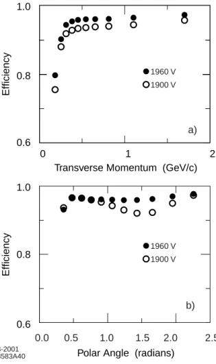
4.1 The PEP-II storage-ring facility located at SLAC. . . 19 4.2 The total integrated luminosity delivered by PEP-II and recorded byBABAR. 21 4.3 The BABARdetector. . . 22 4.4 The orientation of the five SVT layers. . . 24 4.5 The SVT resolution in both (a)z, and (b)φas a function of incident angle. . 24 4.6 Cross-sections of the drift chamber. . . 26 4.7 The efficiency of track reconstruction as a function of transverse momentum
and polar angle at two DCH voltages. . . 27
4.8 ThedE/dxdistribution as a function of momentum as measured by the DCH.
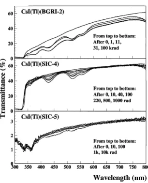
The Bethe-Bloch curves for the different particle types are also shown. . . 28 4.9 The longitudinal cross-section of the DIRC with an example particle included. 29 4.10 The expected Cherenkov angle andK/πseparation using the DIRC information. 30 4.11 The falloff in transmittance for three crystals as a function of absorbed
radia-tion dose. . . 32 4.12 The percent change in light yield over the run of the experiment, plotted with
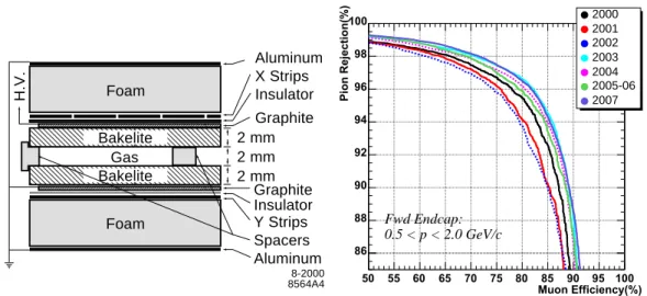
respect to absorbed radiation dose (rad). The different crystal manufacturers are indicated. . . 33 4.13 The schematics of an RPC within the IFR, and the change in performance of
the IFR at distinguishing between µ/π. . . 35 4.14 The efficiency of finding a kaon compared to mis-identifying a different type of
particle as a kaon. The ECOC method is shown in red, the previous methods employing a likelihood selector and single neural network are shown in blue and green. . . 37 4.15 The most important variables used for discriminating between the given
6.1 The source of the high-energy photon from our different types of background events. The y-axis indicates the number of events from these sources. The three stack plots represent: noπ0veto, a simple mass window cut[0.11,0.15] GeV/c2, and a cut on the π0 veto described in the text. . . 45 6.2 The response of the π0 veto classifier to both true π0s and false π0s. The
classifier is constructed to have a response between 0 and 1, 1 indicating more likely for the photon to originate from a π0. A response of -1 indicates the high-energy photon cannot be combined with another photon to form a particle consistent with the π0 mass hypothesis. . . . 46 6.3 Correlation plot of variables used in BRC training. B Momentum Flow
2-17 is omitted from the plot. In the 2D histogram, red represents a higher concentration of signal events and blue represents a lower concentration of signal events. The 1D histograms show signal (red) and background (blue). . 50 6.4 The response of the BRC (x-axis) for background candidates with mES >
5.265 (dashed), background candidates withmES <5.265 (dotted), and signal
candidates (solid line) for run 3 MC. We also compare off peak data (red) to continuum MC (green) for mES < 5.265 (solid) and mES > 5.265 (dashed).
Further details about the normalization of the background are given in the text. 52 6.5 Correlation plot of variables used in SSC training. In the 2D histogram, red
represents a higher concentration of true signal candidates and blue represents a lower concentration of true signal candidates. . . 54 6.6 Normalized distribution of maximum SSC response for both signal and
back-ground events. We show signal MC in which the true signal candidate is selected (red) and in which the wrong candidate is selected (black). . . 55 6.7 A comparison of signal efficiency and background efficiency for the two
meth-ods of choosing the best candidate in the event. We see that using the SSC method, and placing different requirements on the minimum classifier response, is more powerful (higher signal efficiency for equivalent background) than sim-ply minimizing|∆E|(and placing different requirements on its maximum value). 55 6.8 The three variables used in optimizing our signal region requirements, having
chosen the best candidate based on the SSC. In all distributions the blue is
B+B−, the yellow is B0B0, the red iscc, the green isuds, the purple is cross-feed, and the unfilled black line is the signal. The background MC has been scaled to match data luminosity, the signal has been weighted to have the same area as the total background in each plot. . . 57
7.1 The fit to two different mass bins in MC showing all component PDFs includ-ing: signal CB (red solid line), cross-feed Nvs (green dotted), cross-feed Argus (green dashed), peaking BB Nvs (red dotted), and combinatoric Argus (blue dashed). . . 71 7.2 The pure toy study for bin 1.4< mXs <1.5 GeV/c
2. The top row shows the
8.1 The signal MC distribution for each mass region showing the sidebands in each of the classifiers. Where indicated by a red (SSC) or green (BRC) line, we used this value of the classifier to delineate the sideband to limit the signal contribution; if there is no line drawn, the default cut of the classifier is used to define the sideband. . . 76 8.2 The efficiencies for MC (red) and data (blue) and their ratios when comparing
the number of events that pass a given cut on the SSC response in the BRC sideband to the number that pass a cut 0.05 below the signal region cut. The x-axis reflects the cut location on the SSC response. The vertical black line indicates the location of the signal region requirement. . . 78 8.3 The efficiencies for MC (red) and data (blue) and their ratios when comparing
the number of events that pass a given cut on the SSC response in the BRC sideband to the number that pass a cut 0.05 below the signal region cut. The x-axis reflects the cut location on the BRC response. The vertical black line indicates the location of the signal region requirement. . . 79 8.4 The highXs mass bin distributions. . . 81
8.5 The source of the high-energy photon in the BB MC. We have plotted the LundID, which is 111 for a π0 and 211 for an η, the two highest sources shown. We have applied all of our selection cuts in this plot and required
mES>5.27 to restrict our plot to the peaking region of mES. . . 83
9.1 The distribution of the different 38 modes we reconstruct (the mode number is given by the x-axis), normalized to the total number of events within the 38 modes (the total area of each histogram is 1). The dashed purple line is the default setting, the pink thin line is the default shower setting, the other lines are the shower setting using the Field-Feynman fragmentation function with different values for its parameter a. . . 91 9.2 The different incl. values for each mass bin for each of the different settings
for spin-1 hadron formation. Each of these was generated with the phase space hadronization model with the probability of thesquark forming a spin-1 hadron given by the first number in the legend (times 10−2) and the probability of theuquark (ordquark) forming a spin-1 hadron given by the second number in the legend (times 10−2). The default settings are given by a black line, in the middle of the distribution. . . 110 9.3 The different incl. values for each mass bin for each of the different settings
for spin-1 hadron formation. Each of these was generated with the showering quark hadronization model (except for the default setting, given by the black line) with the probability of thesquark forming a spin-1 hadron given by the first number in the legend (times 10−2) and the probability of theuquark (or
d quark) forming a spin-1 hadron given by the second number in the legend (times 10−2). . . . 111 9.4 The reweighting factors predicted by different spin-1 hadron formation
9.5 The reweighting factors predicted by different spin-1 hadron formation probal-ities for showering quarks hadronization generated models in mass region
1.1< mXs <1.5. The x-axis corresponds to the data sets given in Table 9.10;
the default MC setting is a flat line of value 1 in every bin. . . 113 9.6 The reweighting factors in mass region 1.1 < mXs < 1.5 predicted by the
eight extreme models with different probability of spin-1 hadron formation (given as Pr(x=1), where x=s u), as well as the results from the measurement in the data, given in Table 9.10. We also show the thermodynamic model’s predictions, and the default reweight (by definition, 1 in all bins). . . 116 9.7 The reweighting factors in mass region 1.5 < mXs < 2.0 predicted by the
eight extreme models with different probability of spin-1 hadron formation (given as Pr(x=1), where x=s u), as well as the results from the measurement in the data, given in Table 9.11. We also show the thermodynamic model’s predictions, and the default reweight (by definition, 1 in all bins). . . 117 9.8 The reweighting factors in mass region 2.0 < mXs < 2.4 predicted by the
eight extreme models with different probability of spin-1 hadron formation (given as Pr(x=1), where x=s u), as well as the results from the measurement in the data, given in Table 9.12. We also show the thermodynamic model’s predictions, and the default reweight (by definition, 1 in all bins). . . 118 9.9 The reweighting factors in mass region 2.4 < mXs < 2.8 predicted by the
eight extreme models with different probability of spin-1 hadron formation (given as Pr(x=1), where x=s u), as well as the results from the measurement in the data, given in Table 9.13. We also show the thermodynamic model’s predictions, and the default reweight (by definition, 1 in all bins). . . 119 9.10 The value for incl. predicted by our eight extreme models (as well as the
thermodynamics model and default model) for each mass bin. . . 121
11.1 ThemXs spectrum, reported in Table 11.1 (blue) as compared to the previous BABAR“sum of exclusives” analysis results (red). The errors for each analysis’
results include the statistical and systematic uncertainties added in quadrature.139 11.2 The Eγ spectrum, reported in Table 11.1 (blue) as compared to the previous
BABAR“sum of exclusives” analysis results (red). The values shown correspond to BF/100 MeV/c2 when binned in hadron mass (as per Figure 11.1). . . 140 11.3 The fits to the mass bins in 0.6< mXs <1.1 GeV/c
2. . . . 142
11.4 The fits to the mass bins in 1.1< mXs <1.5 GeV/c
2. . . . 143
11.5 The fits to the mass bins in 1.5< mXs <2.0 GeV/c
2. . . . 144
11.6 The fits to the mass bins in 2.0< mXs <2.4 GeV/c
2. . . . 145
11.7 The fits to the mass bins in 2.4< mXs <2.8 GeV/c
2. . . . 145
11.8 The mean (left) and variance (right) distributions used in calculating the error on these quantities. The vertical lines reflect the 16% integrals (68% coverage in the central region). . . 155 11.9 The correlation between the mean (y-axis) and variance (x-axis) when
propa-gating the statistical error at the lowest photon energy cutoff. . . 157 11.10 The kinetic model results. . . 162 11.11 A 3-dimensional rendering of the 1-σ region for the kinetic models. Points
11.13 A 3-dimensional rendering of the 1-σ region. Points with ∆χ2 > 1 are fixed to a shift of 1.. . . 165 11.14 The kinetic model results for the Eγ spectrum and the three-sigma curve. . . 167
11.15 The shape function model results for the Eγ spectrum and the three-sigma
List of Tables
2.1 Different NP models and their effects (relative to the SM) on the transition rate of b → sγ (⇑ indicating an enhancement in the rate), as well as the precision in the respective calculation of the model’s effect. Please see [9] for more details and other model effects. . . 8
3.1 The 38 modes we reconstruct in this analysis; BiType identifies the numeric value we assign to each mode for bookkeeping; charge conjugation is implied. 15
3.2 Numerical conversion from hadron system mass to photon energy. . . 16
4.1 Relevant properties of CsI(Tl) crystals. . . 31 4.2 The cross-sections, production and L1 trigger rates for different physics
pro-cesses at 10.58 GeV and a luminosity of 3×1033cm−2s−1. Thee+e−rate refers to events in which one or both leptons are found in the EMC. . . 35
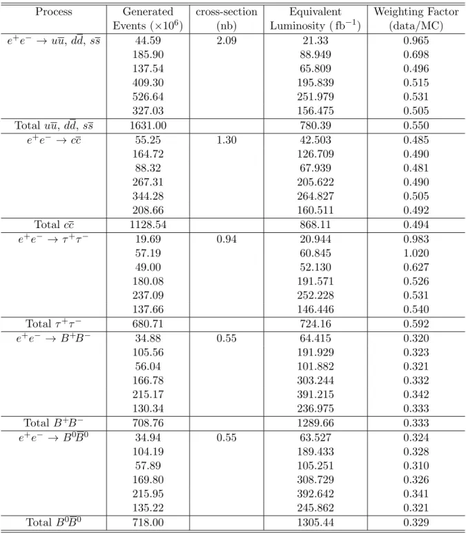
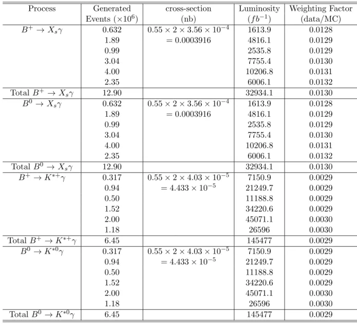
5.1 The run-by-run integrated luminosity of the on peak and off peak data. . . . 40 5.2 The run-by-run number of MC events, cross-section, equivalent luminosity,
and weighting factor for each background mode. . . 42 5.3 The run-by-run number of signal MC events generated and luminosity
weight-ing factors. . . 43
6.1 The final cut requirements in each mass bin for selecting best candidate based on the SSC. . . 57 6.2 The signal and background events in each mass bin, as well as precision, for
the final cuts given in Table 6.1 using the best B candidate taken from the SSC and requiring mES>5.27. . . 58
6.3 The different sources of background events, based on the test MC, scaled to reflect total luminosity, after cuts given in Table 6.1 and selecting the best B
based on the SSC, mES >5.27, and KaonKMLoose requirements. . . 59
6.4 The average B candidate multiplicity by MC type after B candidate recon-struction. These numbers come from run 1 MC. . . 60 6.5 The signal efficiencies for the final cuts in each mass bin when comparing
expected signal yield compared to the amount of our 38 exclusive modes gen-erated within the bin (38). . . 61
7.2 The different shape parameters for the cross-feed Nvs function used to model the peaking component in the different mXs regions. . . 65 7.3 The change in peaking cross-feed when using the Nvs function vs. a CB function. 66 7.4 The different shape parameters for the BB Nvs function used to model the
peaking component in the different mXs bins. . . 67 7.5 The number of peaking BB events in each mass bin. We fix this in the final
fit. The uncertainty reflects the statistical uncertainty of the fit. . . 67 7.6 Summary of fitting functions and parameters; here XF stands for cross-feed.
The order of the table is meant to reflect how we build up to the last fits to On Peak data. “3 or 4 mass regions” refers to groups of mass bins, as shown in other tables; “mass bins” refers to fits done on individual mass bins. . . . 69 7.7 The results in each bin of our fitting procedure, the difference from the actual
value, the uncertainty on the fit, and the associated χ2. . . 70 7.8 The results of the toy studies in each mass bin; we report the mean and sigma
of a Gaussian fit to the pull distributions of the toy-fits to the fractional con-tribution of the signal+cross-feed and the slope parameter of the combinatoric Argus function. . . 72 7.9 The results of the embedded toy studies in each mass bin in which we only
embed signal and cross-feed MC in a PDF-generated background; we report the expected fraction from truth matching as well as the fitted fraction with rms error after 400 studies, and mean of a Gaussian fit to the pull distribution of the fitted fraction. . . 74
8.1 The ratio between MC and data of changes in efficiencies when comparing the signal region cut value to five bins looser than the signal region cut value for each of the classifier sidebands. . . 77 8.2 The ratio between MC and data of changes in efficiencies when comparing the
signal region cut value to five bins looser than the signal region cut value for the sideband with the π0 veto>0. . . . 80 8.3 The different MC components and total amount of data in the 2.9< mXs <3.0 GeV/c
2
bin. . . 82 8.4 The amount of peakingBB expected from a fit to just theBB MC (NBB
BB), a
fit to the full MC set (NBBf ull), and a fit to the data (NBBdata) in theπ0 sideband. We also explicitly report the uncertainty on this fit to the data. . . 84 8.5 The number of peakingBBevents in each mass bin with the uncertainty from
our fit to MC supplemented by the uncertainty from our fit to the data in the
π0 sideband (the uncertainty from the fit to MC is added in quadrature to the uncertainty reported in Table 8.4). . . 85
9.1 The breakdown, by %, of the different missing fraction of events for the default MC settings. The events are generated with a flat photon spectrum in the mass bin, and there is no photon energy reweighting. . . 89 9.2 The breakdown, by %, of the different missing fraction of events for the default
9.3 The breakdown, by %, of the different missing fraction of events for reweighting the events based on the thermodynamics model detailed in the text. The events are generated with a flat photon spectrum in the mass bin, and there is no photon energy reweighting except for the final line in which we assume our
default BBU weights for the photon spectrum. . . 95
9.4 The 10 groups used in our fragmentation study based on mode topology. We only give the mode number, please see Table 3.1 for definitions of the specific modes. . . 98
9.5 The evolution of the weights to be used to better match the MC to the data based on the 10 groups we identified, in mass region 1.5-2.0 GeV for our mock fragmentation study. . . 99
9.6 The weights determined for correcting the MC to match the showering quarks “data” to better determine 38, with the 10 groups we used in our study. . . 101
9.7 The default value for38, as well as the values found from applying the correc-tions based on the weights given above, and the actual showering quarks MC value of 38. . . 102
9.8 The number of events generated in our 38 decay modes predicted by our cor-rected value of38(Ngen−38) and the actual number of events generated in our 38 modes in the showering quarks model of signal MC (Actual SQ 38). . . . 102
9.9 A cross-check to ensure that we can recover the default reconstruction effi-ciency for our 38 modes if we start with the showering quarks effieffi-ciency (SQ 38). . . 103
9.10 The reweighing factors found in mass region mXs=1.1-1.5 GeV. . . 103
9.11 The reweighing factors found in mass region mXs=1.5-2.0 GeV. . . 104
9.12 The reweighing factors found in mass region mXs=2.0-2.4 GeV. . . 104
9.13 The reweighing factors found in mass region mXs=2.4-2.8 GeV. . . 105
9.14 The final shape parameters for the cross-feed Nvs function used to model the peaking component in the different mXs regions after the fragmentation study. 106 9.15 The Argus slope and peaking fraction for the cross-feed after the fragmentation study. . . 107
9.16 The value of 38 before and after the fragmentation corrections. The uncer-tainty on the corrected value reflects the systematic unceruncer-tainty based on the uncertainty of the fits to the data. . . 108
9.17 The models we define as “extreme” for the given mass ranges, used for evalu-ating a reasonable range of fraction of missing final state predictions. . . 115
9.18 The most extreme values for incl. we were able to generate and the model these extremes corresponds to. The default value for each bin is also given. The notation Pr(x=1) refers to the probability for a hadron being generated in a spin-1 state from the quark x(=s,u (d)). . . 122
10.1 The selection efficiency systematic uncertainty in each mass region. . . 124
10.3 The average %-change in signal yield when each parameter is shifted by the values given in the text. The total uncertainty is the sum in quadrature of each of the columns. . . 129 10.4 The %-uncertainty in signal yield from fixing the shape parameters in the
signal+cross-feed PDF. The ρ given reflects the correlation between the pa-rameter and the signal fraction when obtaining the total uncertainty (the correlation between columns 3 and 4 is assumed to be 0). . . 131 10.5 The %-change in signal yield when each parameter of the BB PDF is varied.
The total uncertainty is the sum in quadrature of the components . . . 132 10.6 The total fitting uncertainty reflecting the sum in quadrature of the
compo-nents given. . . 133 10.7 The uncertainty on 38 from each group used in our fragmentation study. . . 135 10.8 Each of these subcomponent uncertainties are assumed to be uncorrelated and
the total reflects their addition in quadrature. All uncertainties are given in %. We have indicated correlated uncertainties between bins with horizontal lines. We motivate these groupings in Section 11.2. . . 138
11.1 The branching fractions of B →Xsγ in each mass bin. These are referred to
as partial branching fractions (PBF). . . 140 11.2 The total systematic errors, each of these subcomponent errors are assumed
to be uncorrelated and the total reflects their addition in quadrature. These reflect the error on the central value reported in Table 11.1. We have indi-cated correlated errors between bins with horizontal lines. We motivate these groupings in Section 11.2. . . 146 11.3 The previous analysis’ results for the PBF in each mass bin. The uncertainties
are statistical and systematic. The total branching fraction is given in the final line. . . 147 11.4 The raw yield, before efficiency correction, found in each mass bin by the
previous analysis with the statistical uncertainties from their fits shown. The final row reflects the raw yield from a fit to all mass bins at once. . . 148 11.5 The variance matrix for two mass bins, given 7 different fully correlated
sys-tematic uncertainties. . . 150 11.6 Correlation coefficient for the systematic errors between mass bins. . . 152 11.7 Correlation coefficient for the total errors between mass bins. . . 153 11.8 The moments of the photon energy spectrum, calculated at multiple photon
energy cutoffs. The errors are statistical and systematic, calculated as de-scribed in the text. . . 154 11.9 The correlation coefficients for the different minimum photon energies based
on statistics uncertainty. . . 157 11.10 The correlation coefficients for the different minimum photon energies based
on systematic uncertainties. . . 158 11.11 The correlation coefficients for the different minimum photon energies based
on total uncertainties (statistical and systematic). . . 158 11.12 The branching fraction for b→sγ extrapolated to a minimum photon energy
Chapter 1
Introduction
BABAR, a particle physics collaboration and detector, located at the Stanford Linear Ac-celerator Center (SLAC), studies flavor physics through weak decays of the B meson by
colliding positrons and electrons with a center-of mass (CM) energy corresponding to the
Υ(4S) resonance. This bottomonium resonance decays almost exclusively to BB pairs,
which then decay to final states consisting of lighter hadrons, leptons, or photons.
Operat-ing at this resonance in “factory mode” for roughly 9 years gave the BABAR collaboration a large data set ofB mesons, which may then be used to constrain different aspects of the
standard model (SM).
The primary purpose of BABAR was to study CP violation in the b sector, potentially responsible for the matter-antimatter asymmetry we see in nature. The large amount ofB
meson data acquired, however, allows for other precision tests of the SM as well. In this
analysis, we perform a measurement of the transition rate of b→ sγ and spectrum of the
photon using the entire BABAR data set. The results presented within are an update of a previousBABARanalysis using roughly one-fifth the data [1].
The procedure for this analysis is similar to many otherBABARanalysis. We reconstruct theB mesons in the recorded events based on the tracks and neutral particles detected. We
then remove the events that are background to ourb→sγ measurements while striving to
maintain adequate efficiency for the b → sγ events themselves. To do this, we use many
of the kinematic variables associated with the detected particles, variables associated with
the reconstructed intermediate states, and overall event topology variables, and feed them
analysis are:
∆E≡EB∗ −√s/2, (1.1)
mES ≡
q
(√s/2)2−P∗2
B, (1.2)
where EB∗ and PB∗ are the reconstructedB meson candidate’s energy and 3-momentum in the CM system. These variables should peak at 0 and the B meson mass respectively for
a correctly reconstructed B meson. We incorporate ∆E, as well as several other variables,
in our multivariate classifiers, and extract the signal yield by fitting the mES distribution.
We choose to use mES, the beam-energy-constrained mass, instead of the closely related
variableminv., or the invariant mass of the reconstructedB based entirely on the measured
momenta and energies of the final state particles, because of the better precision of mES
and this variable’s minimal correlation with ∆E. We extract our signal yield in bins of
the Xs-hadron mass,mXs, and use the measured values of the partial branching fractions in each of these bins to determine a total transition rate for the decay b → sγ, and then
Chapter 2
Theory
The SM describes the interactions of particles at the most fundamental level through
pa-rameterizations of three of the four known forces (the SM excludes gravity). Within the
context of the SM, the fundamental particles may be classified as either quarks and leptons,
spin-1/2 fermions, or force-carrying spin-1 bosons. There are six quarks and six leptons,
arranged in three generation pairs. For the quarks these are, in order of increasing
ap-proximate mass, “up-down,” “charm-strange,” “top-bottom,” and for the leptons these are
electron, muon, and tau along with the respective flavor of neutrino. The electroweak and
strong force carriers are the photon (γ),W±,Z, and gluon.
The electroweak force, in particular through itsW±mediators, is responsible for
genera-tion changes (or “flavor changes”) within the SM, resulting in up-and-down-type transigenera-tions
for the quarks. In the quark sector, the coupling between the generations may be succinctly
described by the Cabbibo-Kobayashi-Maskawa (CKM) matrix [2], which parameterizes the
mixing that results from the mass eigenbasis (what we measure) not being identical to the
weak eigenbasis (what is produced). There are several ways one may parameterize this
matrix, a more popular one is the Wolfenstein parameterization [3]:
Vud Vus Vub
Vcd Vcs Vcb
Vtd Vts Vtb
=
1−λ22 λ Aλ3(ρ−iη)
−λ 1−λ22 Aλ2
Aλ3(1−ρ−iη) −Aλ2 1
,
of unitarity on the CKM matrix implies both:
X
k
|Vik|2= 1, (2.1)
and
X
k
VikVjk∗ = 0. (2.2)
This latter constraint allows for a graphical representation in the form of three “unitarity
triangles”; the one most relevant toBABARis shown in Figure 2.1.
Figure 2.1: One of the three unitarity triangles with the Wolfenstein parameters shown.
2.1
b
→
sγ
Transition Rate
The flavor changing neutral current (FCNC) transition b → sγ first occurs at the loop
level within the SM (this is true in general of FCNCs in the SM), and has for a long time
been recognized as an important probe for new physics (NP). Consequently, much work
has gone into calculating the transition rate ofb→sγ, and the current predictions for this
transition rate use the next-to-next-to leading order (NNLO) precision in the perturbative
component [4]. The current world average of the measured branching fraction with a cut
on Eγ>1.6 GeV in the B-rest frame is [5]:
B(B →Xsγ)expEγ>1.6 GeV = 3.55±0.24±0.09×10
where the first error is the statistical and systematic errors combined and the second is due
to extrapolating down to a photon energy of 1.6 GeV based on the input shape function
(the high photon energy limit being equal to mB/2). The total error on this measurement
is about 7.2% of the central value. However, the relation
Γ(B →Xsγ)'Γ(b→Xspartonγ) (2.4)
is valid up to non-perturbative corrections, which are on the order of 5% (and are currently
the largest component of the error in the theoretical predictions at NNLO in the perturbative
expansion discussed below [4]).
Following the NNLO calculation described in [4], [6], and [7], the branching ratio can
be expressed as:
B(B →Xsγ)Eγ>E0 =B(B →Xceν)
Vts∗Vtb
Vcb
2 6αem
πC (P(E0) +N(E0)), (2.5)
where N(E0) denotes the non-perturbative correction differentiating the l.h.s. from the
r.h.s. in equation 2.4. The perturbative contribution to this calculation, P(E0), is taken
from the ratio
Γ(b→Xsγ)Eγ>E0
|Vcb/Vub|2Γ(b→Xueν)
=
Vts∗Vtb
Vcb
2 6αem
π P(E0), (2.6)
and it is this quantity, P(E0), for which one calculates the NNLO QCD corrections. Since
equation 2.6 is normalized to the charmless semileptonic rate, the quantityC is effectively
a “non-perturbative semileptonic phase-space factor,” given by:
C=
Vub
Vcb
2
Γ(B →Xceν)
Γ(B →Xueν)
. (2.7)
With the denominator on the l.h.s of equation 2.6 already calculated to NNLO in [8],
the procedure for extracting the value ofP(E0) proceeds in three steps:
The Ci are effectively coupling constants at the flavor-changing vertices, Qi. TheCi
account for the full QCD theory and are evaluated at some higher-mass
renormal-ization scale, taken to be µ0 ∼ Mw, mt, by requiring equality between the effective
theory and the SM to leading order in (external momenta)/(Mw, mt). The effective
Lagrangian for the NNLO calculation is taken to be [4]:
L=LQCD×QED(u, d, s, c, b) +
4GF √
2
"
Vts∗Vtb
8
X
i=1
CiQi+Vus∗Vub
2
X
i=1
Cic(Qui −Qi)
#
,
(2.8)
where
Qu1 = (sLγµTauL)(uLγµTabL),
Qu2 = (sLγµuL)(uLγµbL),
Q1 = (sLγµTacL)(cLγµTabL),
Q2 = (sLγµcL)(cLγµbL),
Q3 = (sLγµbL)Σq(qγµq),
Q4 = (sLγµTabL)Σq(qγµTaq),
Q5 = (sLγµ1γµ2γµ3bL)Σq(qγµ1γµ2γµ3q),
Q6 = (sLγµ1γµ2γµ3TabL)Σq(qγµ1γµ2γµ3Taq),
Q7 =
e
16π2mb(sLσ
µνb R)Fµν,
Q8 =
g
16π2mb(sLσ
µνTab R)Gaµν.
For completeness, it should be mentioned that the contribution of the last term in the
bracket in equation 2.8 is minimal in the NLO calculation, and expansion to NNLO
in [4] is neglected.
2. Determine how the operators mix under renormalization and evolve the corresponding
Ci(µ) from µ0 down to the appropriate energy scale for the process, taken to be
3. Evaluate theb→Xspartonγ amplitudes atµb ∼mb.
W
u d
c b
W
u d
c b
g
(a) The current-current operators,Qc1,2(c
re-ferring to the bottom quark transitioning to a charm quark, there are similar diagrams for the subsequent charm to strange transition)
b s
W
t t
g, γ
(b) The magnetic penguin opera-tors,Q7(γ),8(g)
Figure 2.2: Typical diagrams in the full theory that lead to the different operators used in calculating the b→sγ branching fraction.
For comparison below to different new physics (NP) models, we summarize one last
aspect of the SM calculation for this transition rate, and that is to point out that the
expression for P(E0) can be written in terms of its perturbative expansion:
P(E0) =P(0)(µb) + ˜αs(µb)
h
P1(1)(µb) +P
(1)
2 (E0, µb)
i
+ ˜α2s(µb)
h
P1(2)(µb) +P
(2)
2 (E0, µb) +P
(2)
3 (E0, µb)
i
+O( ˜α3s),
(2.9)
where
˜
αs≡
α(5)s (µb)
4π , (2.10)
is the strong coupling constant evaluated at the energy scale appropriate for this process,
µb ∼mb. The zeroth order term (as well as some of the higher order terms, see equations
2.8 and 2.11 in [4]) may be fully expressed in terms of a single Wilson coefficient, C7(0)ef f:
P(0)(µb) =
C7(0)ef f(µb)
2
, (2.11)
where the zeroth order in ˜αs effective Wilson coefficient,C7(0)ef f, is defined in equations 2.7
The current NNLO calculated value in the SM forB(B →Xsγ) is (3.15±0.23)×10−4[4],
with a minimum photon energy cutoff of Emin>1.6 GeV. The world-average experimental
result: B(B →Xsγ) = (3.55±0.24±0.09)×10−4[5], consists of measurements that generally
use a photon energy cutoff aroundEmin >{1.8−2.0} to reduce background from other B
events, and extrapolate the result to the cutoff given above.
2.1.1 NP Models and b →sγ
There are many NP models that can either enhance or suppress the transition rate ofb→sγ;
several are summarized in Table 2.1 (this summary is taken from [9], see Table I therein for
further references). We will describe in more detail the effects of two of the more popular of
these models: the two Higgs doublet model (2HDM) type II (“type” referring to the nature
of the couplings of the doublets to the different types of quarks), and a general minimally
super symmetric SM (MSSM). Typical diagrams reflecting the contributions from these
models to theb→sγ transition rate are shown Figure 2.3.
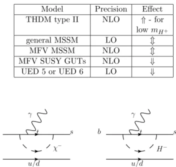
Table 2.1: Different NP models and their effects (relative to the SM) on the transition rate of b → sγ (⇑ indicating an enhancement in the rate), as well as the precision in the respective calculation of the model’s effect. Please see [9] for more details and other model effects.
Model Precision Effect
THDM type II NLO ⇑- for
low mH+
general MSSM LO m
MFV MSSM NLO m
MFV SUSY GUTs NLO ⇓
UED 5 or UED 6 LO ⇓
b
χ−
s t
u/d γ
b
H−
s t
u/d γ
As with most NP models’ effects on b → sγ, the type-II 2HDM would enhance the
transition rate by introducing another amplitude with a charged boson, the H−, replacing
the W− in the loop, as shown in Figure 2.3. The type-II 2HDM (type-II corresponding
to one doublet, referred to asφ1 in [10], coupling to the down-type quarks, and the other
doublet,φ2, coupling to the up-type quarks and leptons), would enhance the value ofC7(0)ef f, given above in equation 2.11. The change due to NP to the b →sγ transition rate at LO
has the form [10]:
P+N = (C7(0),SMef f +B∆C7(0),Hef f− )2+A, (2.12)
where the C7(0)ef f coefficients reflect either the SM Wilson coefficient, or the change intro-duced by the 2HDM. The functions A and B (B being positive) are independent of the
relevant 2HDM parametersmH− (the mass of the new charged Higgs) and tanβ (the ratio
of the two vacuum expectation values,v2/v1). The quantity ∆C7(0),Hef f− does depend on these
parameters (it is related to different powers of the inverse of both of them, and has the
same sign as its SM counterpart, effectively enhancing the transition rate). The measured
rate ofb→sγ therefore provides very strict limits on their values.
The impact of the 2HDM on the transition rate of b→sγ has been calculated to NLO
(see, for instance, [7] or [10]), and, even with the experimental branching ratio ofB →Xsγ
being noticeably higher than the SM prediction, this mode provides one of the strongest
tests of the available parameter space for this model, as shown in Figure 2.4.
However, the 2HDM does not need to be the only source of NP. Indeed, typical SUSY
models imply the presence of a 2HDM component, and an MSSM with minimal flavor
viola-tion (MFV, meaning the FCNC processes are suppressed by the same CKM elements as in
the SM, thus avoiding models that predict increased rates of FCNCs) will have contributions
to theb→sγ transitions from other sources as well.
The impact of the different sources of NP on the appropriate Wilson coefficients in an
MFV MSSM can be written as (neutralino omitted since its contribution is expected to be
small):
(a) The exclusion region of mH+ vs. tanβ (white region excluded at 95% confidence) based on the current experimental value ofB(B→Xsγ). Taken from [10].
(b) The allowed region ofmH+ vs. tanβ(the region allowed by all mea-surements is given in orange) based on the measuredB(B→Xsγ) as well as other measurements. Taken from [10].
which explicitly refers to the SM contribution, the charged Higgs contribution, the chargino
contribution, and the gluino contribution. In such a model, the charged Higgs
contribu-tion still constructively interferes with the SM contribucontribu-tion, but there is no such a priori
requirement on the other terms. Therefore, while in the context of a bare 2HDM, b→ sγ
places strong constraints on the available parameter space, in a typical MSSM with MFV,
the potential for destructive interference between the competing diagrams limits the impact
of b→sγ in parameter determination [11]. Nevertheless, in the context of other
measure-ments, such as the anomalous magnetic moment of the muon, gµ−2, which can also be
strongly impacted by the existence of supersymmetry (and is currently about 2-3σ different
than the SM expectation), regions of parameter space in this class of models can still be
favored more than others. The combination of these two measurements tends to favor both
a light chargino and light charged Higgs as described in [12].
2.2
b
→
sγ
Photon Spectrum
Unlike the total transition rate, the photon energy spectrum is not expected to be heavily
influenced by NP. Nevertheless, measurement of the photon spectrum, and specifically the
moments of this spectrum provides constraints that improve other SM calculations.
At the quark level, the transition b → sγ emits a photon kinematically fixed to Eγ =
mb/2 in the b quark rest frame, where mb is the mass of the b quark. However, two
separate processes contribute to translating this delta function into a photon spectrum in
B → Xsγ. First, what we detect is not b → sγ, but rather b → Xspartonγ, and when
one or more gluons or a qq pair is emitted, the photon is detected with Eγ < mb/2.
Second, there is a “smearing” of the photon energy due to the Fermi motion of the quark
within the B meson. This smearing causes the photon to have a final energy both above
and below the kinematicaly expected value above. The first process may be described by
perturbative QCD, while the second must be modeled by a shape function of the Fermi
motion [13]. This shape function is universal, in that the same shape function describes the
non-perturbative photon spectrum in B →Xsγ and the lepton energy spectrum near the
in the final state (as supposed to B → Xclν). Because of momentum conservation, the
photon has a maximum value of Eγmax = MB/2, where MB is the mass of the B meson,
and the shape function used to model the Fermi motion of the b quark is necessary to
describe the spectrum in a range mb+(MB−mb)
2 > Eγ >
mb−(MB−mb)
2 . As the energy of the
photon gets lower, the perturbative QCD modification of the photon spectrum becomes
more important. For a quark mass ofmb=4.65 GeV/c2, this puts the lower end of the Fermi
motion’s impact aroundEγ ≈2 GeV in theB meson rest frame, which is the recommended
maximum experimental cutoff value given in [15] (i.e. experimental measurements should
use this value or lower for the Eγ minimum cutoff). Others [16] recommend placing this
cutoff no higher than Ecut ≥ 1.85 GeV. Experimentally, however, lower photon energy
cutoffs introduce larger background levels (in particular, backgrounds from other B meson
decays). For this analysis, we place a minimum photon energy cut at Eγ= 1.9 GeV.
As mentioned above, relevant HQET parameters may be extracted from the spectrum
of the photon energy. The parametersmb andµ2π (also called −λ1 in the literature) may be extracted through accurate measurement of the first and second moments. The presence of
a minimum photon energy cut, however, influences the measured values of these parameters.
There are several reasons for placing a cut on the photon energy as low as possible.
First, there are many ways to parameterize the shape function of the Fermi motion of the
b quark; two popular ones include a momentum-dependent product of a power law and
an exponential, and a momentum-dependent product of a power law and a Gaussian (like
the shape functions used in [15], [16], and [17]). The lower the photon energy cutoff, the
less the dependence on the choice of this shape function enters into the extrapolation to
Eγ > 1.6 GeV used in theoretical calculations. By measuring the moments of the photon
spectrum, theorists will be able to determine values to the parameters in whichever shape
function ansatz they choose, and then perform this extrapolation. Second, the lower the
photon energy cutoff, the more accurately the measured moments reflect the actual moments
in the absence of a minimum photon energy cut, and the less biased these measured moment
values become. For instance, in [16], they predict the bias on the moment values based on
µ2π = 0.0790 GeV2 with a photon energy cut at Eγ = 1.9 GeV (assuming central values of
mb(1 GeV) = 4.61 GeV and µ2π(1 GeV) = 0.41 GeV2). Finally, as one lowers the photon
energy cutoff, specific Xs resonances become less important andb→sγ transitions may be
approximated by genericXs hadronization models. Indeed, as recommended by [15], since
the widths ofXs resonances above theK∗(892) exceed their spacing, we will only consider
this specific resonance and model the remainder of the b → sγ transitions with a generic
Chapter 3
Analysis Procedure
There are several ways to perform a measurement of the parton transition b → sγ. For
this analysis, we use the method called “sum-of-exclusives,” referring to the fact that we
reconstruct the s-quark system in one of 38 final states, given in Table 3.1. These 38
modes do not represent an exhaustive list of the final states of the s quark; rather they
reflect that subset of the final states for which we have reasonable detection efficiency and
signal/background separation.
Because we are reconstructing theXs-system (the final hadronic state of thesquark), we
have direct access to the invariant mass of the Xs-system (to within detector resolution),
which we may then translate into a measurement of the photon energy in the b → sγ
transition in theBmeson rest frame (we refer to this as the “transition photon” throughout).
The photon energy is related to the invariant mass of theXs-system through:
EγB= m
2
B−m2Xs 2mB
, (3.1)
where EB
γ is the transition photon’s energy in the B rest frame, mB is the mass of the
Bmeson, andmXs is the invariant mass of theXshadronic system. Therefore, by measuring the spectrum of mXs, we will be able to measure the Eγ spectrum. Since the B mesons are not generated at rest in either the laboratory frame, or the Υ(4S) frame, an accurate
measurement of the photon spectrum in the B rest frame is not as experimentally feasible
with a more “inclusive-measurement” approach. In order to remain as spectrum-model
Table 3.1: The 38 modes we reconstruct in this analysis; BiType identifies the numeric value we assign to each mode for bookkeeping; charge conjugation is implied.
BiType Final State BiType Final State
1 B+→KSπ+γ 20 B0 →KSπ+π−π+π−γ
2 B+→K+π0γ 21 B0 →K+π+π−π−π0γ
3 B0→K+π−γ 22 B0 →KSπ+π−π0π0γ
4 B0→KSπ0γ 23 B+→K+η(→γγ)γ
5 B+→K+π+π−γ 24 B0 →KSη(→γγ)γ
6 B+→KSπ+π0γ 25 B+→KSη(→γγ)π+γ
7 B+→K+π0π0γ 26 B+→K+η(→γγ)π0γ
8 B0→KSπ+π−γ 27 B0 →K+η(→γγ)π−γ
9 B0→K+π−π0γ 28 B0 →KSη(→γγ)π0γ
10 B0→KSπ0π0γ 29 B+→K+η(→γγ)π+π−γ
11 B+→KSπ+π−π+γ 30 B+→KSη(→γγ)π+π0γ
12 B+→K+π+π−π0γ 31 B0 →KSη(→γγ)π+π−γ
13 B+→KSπ+π0π0γ 32 B0 →K+η(→γγ)π−π0γ
14 B0→K+π+π−π−γ 33 B+→K+K−K+γ
15 B0→KSπ0π+π−γ 34 B0 →K+K−KSγ
16 B0→K+π−π0π0γ 35 B+→K+K−KSπ+γ
17 B+→K+π+π−π+π−γ 36 B+→K+K−K+π0γ
18 B+→KSπ+π−π+π0γ 37 B0 →K+K−K+π−γ
19 B+→K+π+π−π0π0γ 38 B0 →K+K−KSπ0γ
events, or signal monte carlo (MC), that are generated with a flat photon spectrum. We
thus obtain a spectrum inmXs that may be translated to a photon spectrum, and used to fit to the best parameter values with any desiredansatz for the photon spectrum. We perform
this analysis using 18 bins of mXs, between 0.6-2.8 GeV/c
2, the first 14 being 100 MeV/c2
wide, the last 4 being 200 MeV/c2 wide. The photon-energy equivalent of the bin boundaries
is given in Table 3.2.
The relevant quantities needed to extract the values of different HQET parameters
are the moments of the photon distribution, as well as the branching fractions in bins of
hadronic mass. We will also report the sum of these branching fractions to derive a total
branching fraction for B → Xsγ with Eγ >1.9 GeV. Finally, we fit the parameters in the
specific models created by [16] and [17] based on our measuredmXs spectrum to determine values formb and µ2π used by [16] (or Λ≡(MB−mb)lim. mb→∞ and µ
2
π for [17]). It should
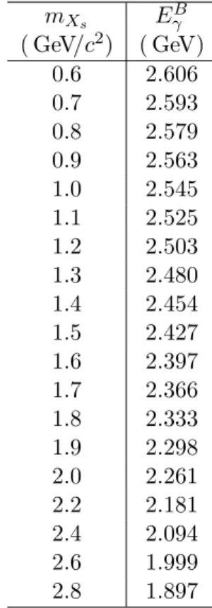
Table 3.2: Numerical conversion from hadron system mass to photon energy.
mXs E
B γ
( GeV/c2) ( GeV)
0.6 2.606
0.7 2.593
0.8 2.579
0.9 2.563
1.0 2.545
1.1 2.525
1.2 2.503
1.3 2.480
1.4 2.454
1.5 2.427
1.6 2.397
1.7 2.366
1.8 2.333
1.9 2.298
2.0 2.261
2.2 2.181
2.4 2.094
2.6 1.999
these models. For the models in [16], the bias in our photon spectrum’s moments have been
evaluated, normalizing the heavy quark parameters atµ= 1 GeV. For the models from [17],
these quantities have been evaluated atµ= 1.5 GeV, and assume a photon energy cutoff of
1.8 GeV. For both of these reasons, the resulting quantities are not immediately comparable.
The branching fractions and moments we report, however, are independent of a particular
Chapter 4
PEP-II and the
B
A
B
AR
Detector
In this chapter we will briefly describe the SLAC B Factory complex, consisting of the
PEP-II collider, used to produce a large sample of BB pairs in e+e− collisions, and the
BABAR detector, used to detect the final state particles of these collisions and reconstruct the decayingB mesons.
4.1
PEP-II
The PEP-II electron-positron collider [18] was a two-ring, high-luminosity collider located
at SLAC (see Figure 4.1), operating at the Υ(4S) resonance. The two-ring system consists
of a high-energy storage ring (HER), 2.2 km in circumference, that delivers electrons at
an energy of 9.0 GeV, and a low-energy storage ring in the same tunnel, that delivers
positrons at an energy of 3.1 GeV. Together, these result in a center of mass (CM) energy
at Interaction Region 2 (where theBABARdetector is located) of√s=10.58 GeV, the mass of the Υ(4S) resonance.
The 3km long SLAC linac provides electron and positron beams to fill the 1658 bunches
at an injection rate of up to 60 Hz. Due to the need for ‘factory’ operating conditions,
consistency in beam intensity is also achieved through continuous injection, or “trickle
charge” mode. The peak instantaneous luminosity achieved by PEP-II during the run of
the experiment was ∼12 nb−1 s−1, about 4×the designed luminosity.
Figure 4.1: The PEP-II storage-ring facility located at SLAC.
Υ(4S)) = 1.1 nb. At this CM energy, however, several other physics processes occur,
including lighter quark pair production: σ(e+e− → uu) = 1.39 nb, σ(e+e− → dd) =
0.35 nb, σ(e+e− → ss) = 0.35, and σ(e+e− → cc) = 1.30 nb; lepton pair production:
σ(e+e− → µ+µ−) = 1.16 nb, and σ(e+e− → τ+τ−) = 0.94 nb; and Bhabha scattering,
σ(e+e−→e+e−)≈40 nb, within the acceptance of theBABARdetector [19].
In general, these non-bbevent types serve as background in most analyses involving at
B mesons with the BABAR data set. Therefore, to study this background, a fraction of data is taken 40 MeV below theΥ(4S) peak, which is about 20 MeV belowBB threshold.
The data taken at this lower energy, “off peak” data, may then be used to characterize the
backgrounds from the competing background processes with noB meson contamination.
Though it is not the focus of this analysis, a brief motivation for the asymmetric ring
energies should be included. The Υ(4S) rest frame, with 9 GeV e− and 3.1 GeV e+, has
a Lorentz boost of βγ = 0.56 with respect to the laboratory frame [20]. This boost is
products of the Υ(4S) (the Υ(4S) decays to a BB pair > 96% of the time [21]). The
average flight distance in the laboratory frame, ∆z, of a B meson, having a mean lifetime
of τ = 1.525×10⁻¹² s, is ∆z = cβγτ ≈ 250µm, well within the resolution of the silicon
vertex tracker (SVT), as discussed below (section 4.2.1). This resolution in decay vertices
allows for the study of time-dependentCP asymmetries between the two, distinguishable,
B mesons, and, using decays such as B0 → ccK(∗)0, yields very precise measurements of
quantities such as sin2β and |λf|[22] (β was introduced in Figure 2.1 andλf relates to the
ratio of theCP-conjugate amplitudes).
The PEP-II facility also ran for extended periods of time at the lower-mass resonances
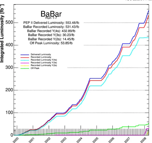
Υ(3S) and Υ(2S), as shown in Figure 4.2, as well as, for a brief period, scanning
ener-gies above the Υ(4S). Ultimately, PEP-II delivered a luminosity of 553.48 fb−1, of which
531.43 fb−1 were recorded by the BABARdetector. 432.89 fb−1 were recorded at theΥ(4S) resonance and 53.85 fb−1 were recorded at the off-peak energy. This analysis uses 429
fb−1 recorded at theΥ(4S) (on-peak data), corresponding to (471.0±1.3)×106 produced
BB pairs, and 44.81 fb−1 of off-peak data. This luminosity corresponds to BABAR data collection runs 1-6, collected between 1999-2008.
4.2
The
B
AB
ARDetector
The BABAR detector [20] is a multi-system particle detector, optimized for the study of
B meson decays, using the high-luminosity asymmetric energy B Factory at PEP-II. The
BABAR detector is composed of five subdetector systems. These are, in order of increas-ing radial distance from the interaction point (IP): the SVT, the drift chamber (DCH),
the detector of internally reflected Cherenkov light (DIRC),the electromagnetic calorimeter
(EMC), and the instrumented flux return (IFR). The first four of these systems are located
within a superconducting solenoid that provides a 1.5 T magnetic field. A schematic of
the detector is shown in Figure 4.3. The data acquisition system (DAQ) provides event
triggering, data readout, and detector control and monitoring.
The BABAR coordinate system is right-handed, with an origin at the nominal IP. The
Scale
BABAR Coordinate System
0 4m
Cryogenic Chimney
Magnetic Shield for DIRC
Bucking Coil Cherenkov Detector
(DIRC)
Support Tube
e– e+
Q4 Q2
Q1
B1
Floor y
x z
1149 1149
Instrumented Flux Return (IFR))
Barrel
Superconducting Coil
Electromagnetic Calorimeter (EMC)
Drift Chamber (DCH) Silicon Vertex Tracker (SVT)
IFR Endcap Forward End Plug 1225
810 1375
3045
3500
3-2001 8583A50
1015 1749
4050
370 I.P. Detector CL
IFR Barrel
Cutaway Section
Scale
BABAR Coordinate System y
x z
DIRC
DCH
SVT
3500 Corner Plates
Gap Filler Plates
0 4m
Superconducting Coil
EMC
IFR Cylindrical RPCs
Earthquake Tie-down
Earthquake Isolator
Floor
3-2001 8583A51
y-axis points vertically upward; and thex-axis points horizontally outward from the center
of the storage rings.
4.2.1 Silicon Vertex Tracker
The SVT is one of the two components that make up the charged particle tracking system,
the other being the DCH (see section 4.2.2). For high-multiplicity final states of thesquark
system in b → sγ transitions, the high efficiency of the BABAR particle tracking system is critical. The SVT measures the positions of charged particles and decay vertices just outside
of the beam pipe using five layers of double-sided silicon strip detectors with readout at
each end to minimize the amount of inactive material in the acceptance volume of the entire
BABARdetector. The silicon strips on each side of the five layers are oriented orthogonally to each other with the φ measuring strips running parallel to the beam axis and the z
measuring strips oriented transverse to the beam axis.
Since the SVT is the detector component closest to the IP, it must provide stand-alone
tracking for low transverse momentum, pt, particles; in the 1.5 T magnetic field of the
solenoid, particles with pt < 120 MeV/c cannot be reliably measured in the DCH alone.
The SVT also provides the best measurement of track angles, essential for more accurate
particle identification (PID) using the Cherenkov angle in the DIRC (see section 4.2.3).
From the inner layer outward, the five layers consist of 6, 6, 6, 16, and 18 modules,
respectively, as shown in Figure 4.4. In total, there are approximately 150,000 channels
read out from the SVT. For this analysis, the precision of the vertex location is less crucial,
but PID is very important (for exampleK/πidentification is crucial for identifying the final
state of the s quark). Since each layer of the SVT is double-sided, there is a potential for
ten signals from a given charged particle, and, because the readout mechanism consists of
a “time over threashold” reading that is a quasi-logarithmic function of collected charge,
there is the potential for ten measurements of dE/dxper track that may be used in PID.
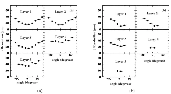
The resolution performance in bothzand φas a function of incident angle for the SVT
Beam Pipe 27.8mm radius
Layer 5a
Layer 5b
Layer 4b
Layer 4a
Layer 3
Layer 2
Layer 1
Figure 4.4: The orientation of the five SVT layers.
Layer 1
Layer 3
Layer 5
Layer 2
Layer 4 (a)
angle (degrees)
angle (degrees)
z Resolution (
μ
m)
(a)
angle (degrees)
angle (degrees)
φ
Resolutiion (
μ
m)
(b) Layer 1 Layer 2
Layer 3 Layer 4
Layer 5
(b)
4.2.2 Drift Chamber
The BABAR DCH complements the SVT measurements of charged particle tracking and identification. It also is the sole source of information on particles that decay outside of
the SVT, such as the KS0 mesons used in this analysis, and therefore measures not just transverse momenta and positions, but also longitudinal positions of the tracks.
The DCH extends for almost 3m along the BABAR detector’s z-axis (see Figure 4.6a), and is composed of 40 cylindrical layers of small hexagonal cells, extending from roughly
0.2-0.8m away from the IP, allowing for up to 40 spatial and ionization loss measurements
for charged particles with transverse momentum greater than 180 MeV/c. To provide
longi-tudinal position information, 24 of the 40 layers are oriented at small stereo angles around
thez-axis. The 40 cylindrical layers are grouped by 4 to create 10 superlayers, which have
either axial alignment, A, (no angle with respect to the z-axis), or a small positive or
neg-ative stereo angle with respect to the z-axis, U and V. These superlayers are arranged in
the order AUVAUVAUVA, moving away from the IP (see Figure 4.6b).
In total, there are 28,768 field, sense, and guard wires, arranged to create 7,104 drift
cells, enclosed in a gas mixture that is 80% helium and 20% isobutane. The chosen gas
has a radiation length that is five times larger than argon-based gases, and the entire DCH
apparatus accounts for less than 0.2% of a radiation length.
Together, the SVT and DCH measurements allow for the reconstruction of charged
particle tracks; each track being defined by five parameters (d0, φ0, ω, z0,tanλ), measured
at the point of closest approach to thez-axis. d0 is the distance of this point from the origin
in the x−y plane, z0 is the distance from the origin along the z-axis, the angle φ0 is the
azimuth of the track, λ is the dip angle relative to the transverse plane, and ω = 1/pt is
its curvature. The fitting algorithm searches the hits in both the SVT and DCH layers to
find tracks, then iterates over the remaining hits to determine if any of these are consistent
with a charged particle track. The efficiency of the fitting algorithm for tracks in the
DCH as a function of transverse momentum and polar angle are shown in Figure 4.7. The
drop in efficiency for finding charged tracks at low transverse momentum is due to limited
IP
236
469 1015
1358 Be
1749
809
485
630 68
27.4
464 Elec–
tronics
17.2
e– e+
1-2001 8583A13
(a) Longitudinal cross-section of the DCH with principal dimensions.
0 Stereo 1
Layer
0 Stereo 1
Layer
0
2 0
2 0
2
0 3
0
4 0
4
45
5 45
5
47
6 47
6 47
6
48
7 48
7
50 8
-52 9
-54 10
-55 11
-57 12
0
13 0
13
0
14 0
14
0 15
0 16
4 cm
Sense Field Guard Clearing
1-2001 8583A14
(b) Layout of drift cells for the four innermost superlayers (lines between filed wires have been added to aid visualization of the cell boundaries).
measurements combined, the uncertainty on the transverse momentum measurement is (pt
is measured in GeV/c):
σpt/pt= (0.13±0.01)×pt% + (0.45±0.03)% (4.1)
Also crucial to this analysis, both the DCH and SVT make measurements of a particle’s
ionization loss per unit track length, dE/dx. This variable follows the Bethe-Bloch
distri-bution, which depends on both particle mass and momentum. ThedE/dxmeasurement in
each of these systems, shown for the DCH in Figure 4.8, is crucial for PID, in particular for
low-momentumK/π identification, and can be used to compute the likelihood for different
particle hypothesis.
Polar Angle (radians) Transverse Momentum (GeV/c)
Efficiency
0.6 0.8 1.0
0.6 0.8 1.0
Efficiency
0 1 2
3-2001 8583A40
1960 V
1900 V
a)
1960 V
1900 V
b)
0.0 0.5 1.0 1.5 2.0 2.5
dE/dx vs momentum
103 104
10-1 1 10
Track momentum (GeV/c)
80% truncated mean (arbitrary units)
e
μ
π
K
p
d
BABAR
Figure 4.8: ThedE/dxdistribution as a function of momentum as measured by the DCH. The Bethe-Bloch curves for the different particle types are also shown.
4.2.3 Detector of Internally Reflected Cherenkov Light
The DIRC subdetector (shown schematically in Figure 4.9) is composed of a 12-sided,
cylindrically symmetric, polygon barrel of 144 synthetic fused silica bars, each side of the
polygon being composed of 12 bars glued together, and optically isolated from the other
sides of the polygon. The DIRC provides PID for higher-momentum particles. The idea
behind the DIRC relies on the Cherenkov radiation’s opening angle remaining constant as
the photons are internally reflected along the length of the DIRC bars until they are read
out by an array of 10,752 photo-multiplier tubes (PMTs) set at the end of the detector away
from the boost. As charged particles, detected by the tracking systems described above,
enter the DIRC, they emit Cherenkov photons that are read by the PMT array. A time
window of±300 ns around the trigger is imposed to cut down on the flat photon background
detected by the PMTs. A vector, pointing from the center of the PMT to the center of the
bar end, is extrapolated into the radiator bar, giving both θc, the Cherenkov angle of the
emitted photons, and φc, the azimuthal angle of the Cherenkov photon around the track
forward or backward, and reflection or no-reflection in the wedge shown in Figure 4.9). By
then turning to the timing information associated with the difference between the PMT
detection time and expected photon arrival time, ∆t, the ambiguity in photon angles is cut
down from 16 to generally 3. Timing information also removes background photons that
are either accelerator-induced or come from other tracks by a factor of approximately 40.
Mirror
4.9 m 4 x 1.225m Bars glued end-to-end
Purified Water
Wedge Track
Trajectory 17.25 mm Thickness
(35.00 mm Width)
Bar Box PMT + Base 10,752 PMT's
Light Catcher
PMT Surface
Window
Standoff Box
Bar
{
{
1.17 m
8-2000 8524A6
Figure 4.9: The longitudinal cross-section of the DIRC with an example particle included.
Due to the asymmetric energies of the beams, the majority of Cherenkov radiation is
emitted in the front end of the DIRC bars. Approximately 28 photoelectrons are expected
for a β = 1 particle entering normal to the surface at the center of the bar, increasing by
more than a factor of two in the forward and backward directions. The resolution on the
measured Cherenkov angle for a given track,σC,track, scales as:
σC,track =
σC,γ
p
Npe
, (4.2)
where σC,γ is the single photon Cherenkov angle resolution, and Npe is the number of
detected photoelectrons. To preserve as many of the Cherenkov photons as possible, mirrors
are inserted at the front end of the bars, allowing for the readout on the opposite end
and greater coverage by other components (such as the EMC) in front of the boost. The
measured Cherenkov angle can be combined with the measured particle momentum (from
the tracking detectors discussed above) to determine a likelihood of the particle’s type, as
and complements the tracking system’s measurement ofdE/dx.
pLab (GeV/c)
θC
(mrad)
e
μ
π
K
p
650700 750 800 850
0 1 2 3 4 5
(a) The expected Cherenkov angle for different particle species at different momenta.
0 2 4 6 8 10
2 2.5 3 3.5 4
momentum (GeV/c)
π
-K separation (s.d.)
BABA R
(b) The performance ofK/πseparation (Nσ sep-aration) for different momenta
Figure 4.10: The expected Cherenkov angle andK/π separation using the DIRC informa-tion.
4.2.4 Electromagnetic Calorimeter
The EMC is composed of 6,580 CsI(Tl) crystals to provide energy and angular resolution
for photons and electrons, over a range of 20 MeV to 9 GeV. The properties of CsI(Tl) are
given in Table 4.1. The crystals are arranged to provide full azimuthal angle coverage, and
polar angle coverage from 15.8◦ to 141.8◦, corresponding to 90% coverage in the center of
mass frame. 5,760 crystals are arranged in 48 distinct rings of 120 crystals each, forming a
cylinder around the interaction point, constituting the barrel region, while 820 crystals are
arranged in 8 rings on a circular structure in front of the boost direction, constituting the
end-cap.
The crystals range in lengths from 16-17.5 radiation lengths, depending on polar angle
location, and are arranged with azimuthal symmetry. To minimize preshowering of the
par-ticles, the amount of material in front of the crystals (from other subdetector components)
is minimized, and is in general between 0.3-0.6 radiation lengths. The light from the EMC