The Error Analysis Based on the Kalman Gain in a Position Predicting Algorithm of an Occluded Object

http://www.scirp.org/journal/jsip ISSN Online: 2159-4481 ISSN Print: 2159-4465

The Error Analysis Based on the Kalman Gain

in a Position Predicting Algorithm of an

Occluded Object

Manaram Gnanasekera, Hansi K. Abeynanda

Sri Lanka Institute of Information Technology, Malabe, Sri Lanka

Abstract

Detecting occluded objects is a crucial exercise in many spheres of application. For example in Strafing (attacking ground targets from low flying aircrafts) or vehicular tracking, continuous detection of the object even when it is occluded by another object is essential. Failing to track the occluded object may result in completely losing its location or another object to be mistakenly tracked. Both of which will result in disastrous consequences. There are various me-thods to handle occlusions. In a previous research which was done by the au-thor, a novel noise filtration mechanism based on the corrector equation of the Kalman filter which can be used with greater accuracy to handle lengthy occlusions was made. In this presentation, a further analysis of the error of the algorithm will be presented. The algorithm when compared with existing al-gorithms under the same test conditions gives promising results.

Keywords

Kalman Filter, Computer Vision Based Tracking, Occlusion

1. Introduction

Occlusion has been a topic of interest in the arena of computer vision for many

years [1] [2] [3] [4]. Occlusion is defined as a situation in which an object gets

covered partially or fully by another object. For Computer Vision based tracking if the object is partially or fully covered by another object, the tacking algorithm can fail. Therefore, it cannot be re-tracked once it reappears after the occlusion period. The reason for this failure is that the motion algorithms are developed for short displacement tracking of objects. Hence when an object disappears from the tracker and reappears, especially after a long duration, the tracking algorithm more or less fails with the existing methods. For the purpose of this

How to cite this paper: Gnanasekera, M. and Abeynanda, H.K. (2017) The Error Analysis Based on the Kalman Gain in a Position Predicting Algorithm of an Oc-cluded Object. Journal of Signal and In-formation Processing, 8, 161-177.

https://doi.org/10.4236/jsip.2017.83011

Received: June 7, 2017 Accepted: August 19, 2017 Published: August 22, 2017

Copyright © 2017 by authors and Scientific Research Publishing Inc. This work is licensed under the Creative Commons Attribution International License (CC BY 4.0).

http://creativecommons.org/licenses/by/4.0/

research, full occlusion is when the entire object is covered for a duration of time and partial occlusion is when only part of the object is covered during the entire occlusion period.

It is important to understand the reason to handle an occlusion. When an object which is tracked gets occluded, the tracker will no longer be able to locate the object. As a result, either the tracking will fail and the object location will be lost or a similar kind of object could be mistakenly tracked instead. Both of which can have disastrous consequences depending on the application. As an example, a UAV (unman aerial vehicle) which tracks a mobile target moving on the ground from the sky is considered. The task of the UAV is to engage the target. While tracking, if the target goes inside a tunnel, the vision-based tracking mechanism will be unable to detect the target. Even if the target appears from the other side of the tunnel, depending on the occlusion duration, the UAV will be unable to track the object. On the other hand, if there was a similar kind of an object at the starting point of occlusion (starting point of the tunnel), that object will be mistakenly tracked instead of the original target. If the UAV engages, it will be the wrong target. However, if there had been a mechanism to track the target during the occlusion period, the correct target would have been engaged despite the occlusion.

There are various algorithms and techniques developed for occlusion handling. One famous way which is applied in occlusion handling of pedestrians is by tracking different body parts of the pedestrian separately by using separate

contours [1] [2] [3] [4]. If one of the parts is occluded and cannot be tracked,

using the other visible trackers, the object will be located. The downfall of this method is that it only works for partial occlusions. If the object is fully occluded, non of the trackers will be able to locate it. The second, not so famous method is

by using multiple cameras to handle occlusions [5] [6] [7] [8]. The benefit of

algorithm will try to keep a track on both the objects together [9] [10] [11] [12]

[13]. This algorithm will work well for a moving object and a moving

foreground object (the object which covers the interested moving object), but for a static foreground object, this technique will be inappropriate. As an example, if the foreground object is a wall (large static foreground object), the object might still be moving behind the wall but the trajectory of the object cannot be tracked with this technique. The final and the most suited method to handle an occlusion of a moving object is by using a type of a Recursive Bayesian Filter. They are used to estimate the future value of a certain property, given the current value of it. Therefore, if the position, velocity and acceleration of the object is known before occlusion, all three properties could be estimated during occlusion. The Kalman filter and the Particle filter are two algorithms which are developed based on the Recursive Bayesian filter. These two algorithms are strictly used for solving the occlusion problem of moving objects. The specialty of the Particle filter is due to the fact that it could be used in both linear and

non-linear systems [14] [15] [16]. However, the Particle filter has its own

limitations, such as Particle Depletion. Particle depletion happens when the required amount of samples are not enough to identify the measured signal. As a result of Particle depletion, an incorrect signal will be identified instead of the correct measured signal. Furthermore, if the measured signal has a lot of noise, due to lack of filtration of the Particle filter, an incorrect signal will be identified by the samples and as a result, the estimation will be incorrect. Therefore, the focus was dragged towards the Kalman filter, which is the other method that is used to handle occlusions of a moving object. There are two phases of the Kalman filter, one which estimates the next state and the other which does the

actual filtering named as the Correction phase. Methods given in [17] [18] [19]

uses the Estimation equation to predict the position during occlusion. However, these existing methods which are developed for occlusion handling carry an error due to lack of noise filtration. In fact, these methods are designed for a relatively small occlusion duration. When these methods are used to handle large occlusions, the error due to noise accumulates. As a result, the algorithm will not be able to re-track the object when it reappears after a large occlusion. This is due to the absence of the correction stage.

In the paper which was previously published by the author [20], it was proved

that the existing Kalman filter based estimation method’s noise filtration has not been adequately addressed and hence error accumulates for lengthy occlusions. Moreover, if the object is accelerating, the error is accumulated faster, com- pounding the problem. Therefore, a novel filtration mechanism based on the

corrector equation of the Kalman filter was proposed in [20]. As opposed to the

existing research which assumes the velocity is constant during the occlusion

period, the proposed algorithm in [20] relaxes this assumption to handle

In this presentation, an in-depth analysis which explains the reasons to get

such promising results in [20] will bring forward. Moreover, the algorithm has

been further tested by conducting experiments to further prove its accuracy. To estimate the position of an object during occlusion, an equation was proposed in

[20]. Section 3 summarizes the work carried out in [20]. In Section 4, the

filtering phase of the algorithm will be discussed with a detailed description given about the selection of the Kalman Gain. In Section 5, the results obtained by the proposed algorithm will be summarized. It will also be shown that the proposed algorithm is better than the existing methods. Finally, the next section concludes this work with few final remarks.

2. The Proposed Algorithm Framework

In the discussion done in [20], the existing occlusion handling method was

named as the “Estimation method”. Firstly this method was investigated for errors when used to handle lengthy occlusions and it was found that the estima- tion method accumulates a large error. Further more, when acceleration is intro- duced to the system the error is magnified compounding the problem. Equation (1) shows the estimation when acceleration is introduced to the system and when it is used to handle lengthy occlusions:

( )

( )

( )

( )

( )

1 1 1 1 1

1 1

2 2

t t t t t t

z = ∆t z₋ + ∆t z₋ +__ ∆t _n₋ + ∆t n₋ +m₋_

 

 

  _{ }

  (1)

In this equation zt−1 signifies the actual displacement, nt−1 is the error due

to acceleration, nt−1 is the error due to velocity. The process noise of the system

is given by mt−1. It was proved that due to these error components the

estimation method was not suitable to handle a full and lengthy occlusion of an accelerating object.

With the aid of the equations of the correction stage of the Kalman Filter, [20]

proposes a noise filtering mechanism as a solution for the error accumulation. The equation of this mechanism has been given in (2):

(

)

ˆ_t ˆ_{t t t} ˆ_t

z =z−+k z + −n z− (2)

The above found ˆzt is a corrected or a filtered value, which is used to

estimate the next state:

( )

( )

( )

1

1

ˆ ˆ ˆ

2

t t t

z−+ = z ∆ +t z ∆t (3)

By considering Equations (2) and (3) the following equation has been

constructed. Where, ∆ = + −z_t z_t n_t zˆ_t−, zˆ_t− is the estimated velocity, zˆ_t is the

corrected velocity, k is the Kalman gain:

( )

( )

( )

[ ]

[ ]( )

1

1 1

ˆ ˆ ˆ

2 2

t t t t t

z−+ = z− ∆ +t z− ∆t +k∆ ∆ +z t ∆z ∆t 

 

  _{  (4)}

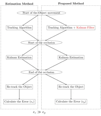
The Block Diagram in Figure 1 summarizes the entire algorithm which was

presented in [20].

Figure 1. Block diagram.

be analyzed in depth. Therefore, we will perform a further analysis of “Kalman Gain” in section four.

3. Analysis of the Kalman Gain and the

Pre-Occlusion Tracking Time

The Kalman Gain brings a major importance for the correction stage of the Kalman filter. Therefore it is important to make an investigation about the Kalman Gain, its minimum and maximum values and the effect it makes to the proposed equation. An expression will be derived from the first basics in order to find the minimum and the maximum values of the Kalman Gain.

3.1. Maximum and Minimum Values of the Kalman Gain

could be given as in Equation (5):

ˆ

t t t

e = −z z (5)

The error could be positive or negative. It could be squared in order to elimi- nate the sign of the error. Even though squaring is possible for the proposed algorithm because there is only one state variable, in general Kalman filters have two or three state variables (which means there will be two or three elements in

the Kalman gain vector). As a result the error will become a vector. In [21], the

error vector is multiplied by its transpose and a squared matrix is made. To increase the accuracy, this multiplication could be done for a number of times and the mean value is taken (this is similar to the expected value).

Due to all the above reasons we will now look at the expected value of the

squared error and it will be called pt:

( )

t t

p =E e (6)

By substituting from Equation (5):

(

)

ˆ

t t t

p =E_ z −z _ (7)

Equation (7) could be expanded by substituting from Equation (2):

(

)

(

)

(

)

ˆ ˆ

t t t t t t

p =E_ z − z−+k z + −n z− _

    (8)

The difference (error) between the actual displacement and the estimated displacement could be given as Equation (9):

ˆ

t t t

e−= −z z− (9)

By substituting from Equation (9), Equation (8) could be further shortened as follows:

(

)

(

)

t t t t

p =E_ e−−k e−+n _

  (10)

Equation (10) could be re-arranged to the following form:

(

)

(

)

1

t t t

p =E_e− −k −kn _

  (11)

By only considering the Corelated terms(unrelated terms will not have a meaning, they are just bi-products of the multiplication) Equation (11) could be re-arranged as follows:

( )

(

)

( )

t t t

b =E_ e− _ −k +E_ n _k

  (12)

Equation (12) could be further shortened by substituting pt E

( )

−  − 

=   and

( )

R= E n _:

2 2

2

t t t t

b =p−− kp−+p k− +Rk (13)

t

b is a squared error term between the actual value and the corrected value.

Therefore k could also be selected in order to minimize b_t. The accepted way

of finding an optimum value (maximum or minimum) is by taking the

derivative. Thereby the optimum k could be found by:

d

2 2 2

d

t

t t

b

p kp kR

k

− −

= − + + ₍₁₄₎

The derivative becomes zero at the optimum value:

0 2pt 2kpt 2kR

− −

= − + + (15)

k could be give by:

t t p k p R − − =

+ (16)

By expanding pt

− _and

R the following equation could be obtained:

( )

( )

( )

E e E n

− −       =  ₊         (17)

The term

( )

t

E_ n _ cannot be negative because this term includes a squared

term of nt. If the measurement noise is zero, nt will be zero. Therefore the

minimum value term

( )

t

E_ n _ could get is 0. When the term E_

( )

zero, k will get the maximum value. The reason is due to the term E_

( )

which is common in both numerator and denominator. Therefore the maximum

value will depend on the

( )

t

E_ n _ term only:

( )

( )

The maximum value of k could be given as:

max 1

k = (19)

The minimum value the term E

( )

−

   

  could get is zero (due to the squared

terms a negative value could not be obtained). Therefore it is obvious that k

cannot be a negative value. As a result the minimum value of k will depend on

the numerator (the minimum value of the numerator is 0):

( )

The minimum value of k could be given as:

min 0

k = (21)

parameters. The kmax value will be applied if there is a zero noise condition and

for the rest of the cases the kmin value will be used. The reason for this is that

we will try to eliminate noise completely when updating the estimation.

Now that the minimum and the maximum Kalman Gain values are known, next, the method of selecting the appropriate Kalman Gain value will be discussed.

At a given state we have two displacement values. One is the measured value and the other is the displacement value estimated in the previous state. The only factor which differs these two values is noise. If not the two values should be the

same. At first, we divide the measurement value ct from the estimated value

ˆt

z− as in Equation (22):

ˆ t

t

c s

z−

= ₍₂₂₎

Ideally if ct and zˆt

− _{has no noise,}

s should be equal to 1. If the values are

largely different from each other the s value will be either smaller or larger

than 1. In this situation either one of the variables or both are having noise. Generally, with more and more samples the estimated value will be getting more closer to expected value (a detailed discussion will be done in the next section). Therefore, it is the measured value we need to control using the Kalman Gain.

When s is larger than a given threshold value, which means there is noise in

the signal, the kmin will be used to eliminate the measurement. If the value is

smaller than the threshold value, we could update the estimate using the maximum Kalman Gain.

As in Equation (23), a is the selected threshold which depends on the en-

vironment. Any s value which is lesser than the threshold will be obtaining the

maximum Kalman Gain. Therefore, a correction for the estimated value could be made. For all the other cases the minimum Kalman Gain value will be app- lied:

max

min

if ,

otherwise

k s a a

k k

 ≤ ∈ℜ

 = 

 (23)

Next, the above found Kalman Gain values will be applied to Equation (4).

The following equation shows the result when k=0 is applied:

( )

( )

( )

1

1

ˆ ˆ ˆ

2

t t t

z−+ = z− ∆ +t z− ∆t (24)

According to the above equation the output depends on the estimated value

only. The correction term is totally ignored. The value 0 for k will be specifically

taken if only the measurement has a large noise and when a proper correction cannot be made. A large measurement noise will make the correction incorrect. In this sort of a situation it is always better to ignore the correction stage of the Kalman filter and only rely on the estimated value of the estimation equation.

very low probability which has the highest noise.

The maximum value of k (k=1) could be only used if the state’s measure-

ment noise is zero. If there is no measurement noise a better correction could be made at the correction stage. This is the best time to make a correction and this corrected value will be much more closer to the actual value in comparison to the state’s estimated value. In the following set of equations the maximum value

of k is applied (k=1):

( )

( )

( )

[ ]

[ ]( )

1

1 1

ˆ ˆ ˆ

2 2

t t t t t

z−+ = z− ∆ +t z− ∆t + ∆ ∆ + z t ∆z ∆t 

 

  _{  (25)}

By expanding the terms ∆zt and ∆zt Equation (25) could be remade as

follows:

( )

( )

( )

( )

1

1 1

ˆ ˆ ˆ ˆ ˆ

2 2

t t t t t t t t t

z−+ = z− ∆ +t z− ∆t +z + −n z−∆ +t z + −n z− ∆t 

 

  _{ }  _{ }  ₍₂₆₎

Due to zero noise at the state, nt and nt terms could be considered as zero:

( )

( )

( )

( )

1

1 1

ˆ ˆ ˆ ˆ ˆ

2 2

t t t t t t t

z−+ = z− ∆ +t z− ∆t +z −z−∆ +t z −z− ∆t 

 

  _  _  ₍₂₇₎

The final result will be as follows:

( )

1 ˆ

2

t t t

z−+ = ∆ +tz z ∆t (28)

When there is no measurement noise the displacement will be equal to the actual value according to (28). This result could be obtained quite often because there will be more occasions where there will be zero noise (due to the Gaussian assumption of the noise distribution).

In general before applying a Kalman filter the behavior of the process noise and the measurement noise should be assumed. Since Gaussian noises with a mean value of zero are allowed in Kalman filters the variance of the Gaussian model should be decided.

It is obvious that there is control over the measurement noise through the thresholding technique in the filtration process. Then, the process noise and the external parameters which make changes to its variance will be discussed in the next section.

3.2. Pre-Occlusion Length and the Process Noise

The process noise is a continuous random variable and we assumed it to have a zero mean Gaussian distribution. As per this reason, in the algorithm proposed in [20] the expected value of the process noise has been taken. According to the Classical Central Limit theorem, the expected value of a set of independent random variables tend towards a normal distribution. As the number of samples increases the variance decreases and the distribution will gain a zero mean value.

The theorem further states that the variance of t number of samples would

have a value of 2

t σ

could be further proved by the Law of large numbers, which says the average number of trials should be close to the expected value. In our situation the expected value is the mean value which is zero.

In summary, when the traveling distance prior to the occlusion increases more and more samples could be obtained for the algorithm. In other words this means that there is a direct proportion between the number of samples and the

distance traveled before the occlusion. Finally, from the expression 2

t σ

we could get the variance when the distance before the occlusion increases.

4. Results and Discussion

In [20], both the algorithms, the proposed method and the estimation method was applied to an object moved in constant velocity and got occluded. Similarly, both the algorithms were applied to an object which moved in constant acceleration and got occluded. In both the experiments it was observed that the proposed algorithm got a low margin of error compared to the estimation method. Firstly, a proper analysis of the obtained result will be done. Secondly given the starting point and acceleration, both of these algorithms will be tested by using different sizes of foreground objects. In Section 4, it was theoretically proved that when the pre-occlusion length increases the error minimizes. Therefore finally the length of the pre-occlusion will be varied and the proposed algorithm will be applied to observe the performance.

The results are categorized in three sections, namely, motion test, performan- ce with different sizes of foreground objects and performance in different starting points.

4.1. Motion Test

The Estimation equation was applied to an object which moves in constant velocity during occlusion. However, it is not practically possible to model an object which moves in constant velocity. There will be a resultant force applied on the object. Hence, the occlusion time was made very small for an object which moved in constant acceleration.

By considering Equation (1), in order to have a very minor occlusion, the time

of occlusion will be given as 0< ∆t1. When the term ∆t gets squared, it

will be more closer to zero. As a result the entire term 1

( )

2 ∆t will be closer to

zero (1

( )

0 2 ∆t ≈ ):

( )

( )

( )

( )

( )

1 1 1 1 1

1 1

0 0

2 2

t t t t t t

z ≈ ∆t z₋ + z₋ +__ _n₋ + ∆t n₋ +m₋_

 

 

  _{ }

  (29)

( )

( )

t t t t

z ≈ ∆t z₋ + ∆_ t n₋ +m_− (30)

There will not be any filtration in this equation and as a result the n and m

error starts increasing. According to the Figure 2 significant increase in error could be observed. Although the occlusion is made small and the acceleration term is eliminated from the equation, the error starts increasing for high accelerations.

Now the same experiment will be conducted for the proposed equation (Equation (3)) and then the results will be observed. The same assumptions will

be made as in the earlier case(0< ∆t1):

[ ]

{

}

( )

{

[ ]

}

1

1

ˆ ˆ 0 ˆ

2

t t t t t

z−₊ = ∆t z−+ ∆k z + z−+ ∆k z (31)

[ ]

{

}

1

ˆ_t ˆ_{t t}

z−+ = ∆t z−+ ∆k z (32)

A very low error value has been observed and during very small accelerations the target point is very close to the actual point. Further reducing the time

period will cause (0< ∆t1) zt ≈0. Which means there is no or there is very

small displacement. When this happens the occlusion will be a partial occlusion and there won’t be a difference between the states.

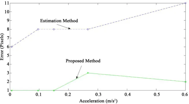
Next the Estimation Equation (1) was applied to an object which was con- stantly accelerating during the occlusion period and the observed results were as in Figure 3. A very large error has been observed in the above graph and it keeps

increasing along with the increase of the acceleration. The mt−1 and nt−1 noise

components are visible in the equation due to lack of filtration. Similarly the experiment was conducted to the proposed algorithm under the same conditions

and results are given in Figure 3. According to the graph the error has reduced

due to the filtration.

4.2. Performance Analysis When Tested with Different

Sizes of Foreground Objects

The size of the foreground object which forms the occlusion is changed and the proposed algorithm and Estimation method (1) will be applied.

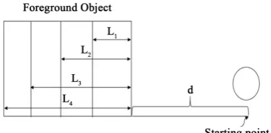
As in the Figure 4 the size of the foreground object will be varied and the

distance to the object’s starting point will be fixed. In addition the object will

Figure 3. Object moving in constant acceleration.

Figure 4. Different sizes of foreground objects.

travel in one common acceleration. The results when the proposed algorithm

and Estimation method were experimented could be given as in Figure 5.

Equation (1) has the error term

( )

( )

1 1 1

1

2 ∆t nt− + ∆t nt− +mt− which will accu-

mulate during the occlusion. This is the main reason for the Estimation method to up-serge the error when the foreground length increases as in the graph labeled as “Estimation method”. Previously it was understood for the proposed algorithm there is no 100% filtration and there will be some noise left. Obviously the noise will cause error and when the size of the foreground object increases, the error will be accumulated. However, the proposed algorithm has a low error in comparison.

4.3. Performance Analysis When Tested with Different

Starting Points

The pre-occlusion time period or in other words the object will be kept in different positions as in the below diagram and the results will be explained in detail. For this test only the proposed algorithm will be used because the Estimation method is not a Markovian type model and has no pre-occlusion

history (Figure 6).

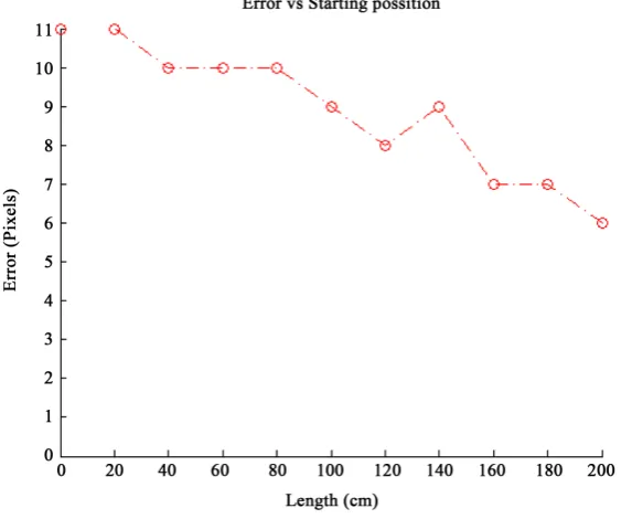
The results of the performed experiment could be given as in Figure 7.

Figure 5. Error vs. length of the foreground objects.

Figure 6. Various starting points.

creases significantly. When the length increases the number of states at the pre- occlusion period will increase and when the states increases more filtering could be done. When there is more filtration more noise cancellation could be done. This is the main reason for the error to reduce when the length increases.

4.4. Effect of the Error

The proposed framework estimates the position of an object (displacement) which is occluded. If one point of the object is tracked prior to the occlusion, the position of the point after occlusion should be same as the position before occlusion. For an example in a face tracking system if the interested point is the

nose as in Figure 8(b) during pre-occlusion, the position of the tracker during

the post occlusion should be pointing on top of the nose as well. If the tracker locates somewhere else other than the nose obviously there should be an error

involved. Figure 8(a) shows the different positions where the location (position)

could be miss tracked during the post occlusion. The red dot locates the correct

position of the nose (Figure 8). The yellow dots around are the possibilities that

the miss tracked locations might occur.

The error is in the form of displacement and the maximum error could be

drawn as in Figure 9. It will be a circle around the actual position and the

maximum error will be the radius of the circle. If the point falls in front of the

line as given in the Figure 9 the error could be taken as a positive value (+) and

if it falls before the line the error could be taken as a negative (−) value.

(a) (b)

Figure 8. Miss-tracked points due to error. (a) Miss-tracked position due to error; (b) Original position of the tracker point.

Due to this reason the error will have a direction and the error accumulation will occur if all the errors happen in one direction.

5. Conclusions

The work undertaken is an extension of the method proposed in [20] by the

author. It has been proved that the maximum and the minimum values of the Kalman gain are 1 and 0. In a heavily noisy condition, the measurement will be incorrect, therefore the Kalman gain value was made zero and that particular measurement will be eliminated. The value 1 for the Kalman gain was assigned when the measurement had no noise. Since there were many states which had zero noise, there were many occasions where the estimated value could be corrected and taken closer to the actual value. The entire estimation procedure during occlusion will depend on the last measurement it takes during the state just before occlusion. Therefore the filtration mechanism will be planted during the pre-occlusion period in order to minimize the error at the last measurement.

The main advantage of this algorithm is that this could be used to handle occlusions which happens for a long time (lengthy occlusion). Absence of filtra- tion will cause an error, which accumulates stage by stage and when the length increases, the output becomes largely erroneous. The effect of the error was explained with aid of a practical face tracking example. Later on, it was proved that the error could be further reduced by increasing the length of the pre- occlusion period. The reason is that when the pre-occlusion length increases, more filtration could be performed.

Significant improvement over the Estimation method’s results were obtained by the proposed algorithm when tested under common conditions.

References

[1] Shu, G., et al. (2012) Part-Based Multiple-Person Tracking with Partial Occlusion Handling. IEEE Conference on Computer Vision and Pattern Recognition (CVPR), Providence, RI, 16-21 June 2012, 1815-1821.

[2] Dinh, T.B. and Medioni, G. (2011) Co-Training Framework of Generative and Dis-criminative Trackers with Partial Occlusion Handling. IEEE Workshop on

Applica-tions of Computer Vision (WACV), Kona, HI, 5-7 January 2011, 13-15.

[3] Enzweiler, M., et al. (2010) Multi-Cue Pedestrian Classification with Partial Occlu-sion Handling. IEEE Conference on Computer Vision and Pattern Recognition

(CVPR), San Francisco, 13-18 June 2010, 990-997.

[4] Ouyang, W. and Wang, X. (2012) A Discriminative Deep Model for Pedestrian De-tection with Occlusion Handling. IEEE Conference on Computer Vision and

Pat-tern Recognition (CVPR), Providence, RI, 16-21 June 2012, 3258-3265.

[5] Fleuret, F., Lengagne, R. and Fua, P. (2005) Fixed Point Probability Field for Com-plex Occlusion Handling. 10th IEEE International Conference on Computer Vision

(ICCV), Washington DC, 17-20 October 2005, 694-700.

[6] Schick, A. and Stiefelhagen, R. (2009) Real-Time GPU-Based Voxel Carving with Systematic Occlusion Handling. Pattern Recognition, 5748, 372-381.

https://doi.org/10.1007/978-3-642-03798-6_38

Using Colored Voxels and 3-D Blobs. 3rd IEEE and ACM International Symposium

on Mixed and Augmented Reality, Arlington, VA, 5-5 November 2004, 266-267.

https://doi.org/10.1109/ISMAR.2004.50

[8] Sun, J., Kang, S.B. and Shum, H.-Y. (2005) Symmetric Stereo Matching for Occlu-sion Handling. IEEE Computer Society Conference on Computer Vision and

Pat-tern Recognition (CVPR), San Diego, CA, 20-26 June, 2005, 399-406.

[9] Senior, A., et al. (2006) Appearance Models for Occlusion Handling. Image and

Vi-sion Computing, 24, 1233-1243.

[10] Pan, J. and Hu, B. (2007) Robust Occlusion Handling in Object Tracking. IEEE

Conference on Computer Vision and Pattern Recognition (CVPR), Minneapolis,

MN, 17-22 June 2007, 1-8. https://doi.org/10.1109/CVPR.2007.383453

[11] Guha, P., Mukerjee, A. and Venkatesh, K. (2005) Efficient Occlusion Handling for Multiple Agent Tracking by Reasoning with Surveillance Event Primitives. 2nd Joint IEEE International Workshop on Visual Surveillance and Performance

Evalu-ation of Tracking and Surveillance, Beijing, 49-56.

[12] Yang, T., Pan, Q. and Li, J. (2005) Real-Time Multiple Objects Tracking with Oc-clusion Handling in Dynamic Scenes. IEEE Computer Society Conference on

Computer Vision and Pattern Recognition, San Diego, 970-975.

[13] Zhong, D., Lu, H. and Yang, M.-H. (2012) Robust Object Tracking via Sparsity Based Collaborative Model. IEEE Conference on Computer Vision and Pattern

Recognition, Providence, 1838-1845.

[14] Schulz, W., Burgard, W. and Craemers, A.B. (2001) Tracking Multiple Moving Targets with a Mobile Robot Using Particle Filters and Statistical Data Association.

IEEE International Conference on Robotics and Automation, Seoul, 1665-1670.

[15] Zhou, S.K., Chellappa, R. and Moghaddam, B. (2004) Visual Tracking and Recogni-tion Using Appearance-Adaptive Models in Particle Filters. IEEE Transactions on

Image Processing, 13, 1491-1506.

[16] Zhang, C., Xu, J., Goto, S. and Beaugendre, A. (2012) A KLT-Based Approach for Occlusion Handling in Human Tracking. Picture Coding Symposium, Krakow, 337- 340.

[17] Panahi, R., Gholampour, I. and Jamzad, M. (2013) Real Time Occlusion Handling Using Kalman Filter and Mean-Shift. 8th Iranian Conference on Machine Vision

and Image Processing, Zanjan, 320-323.

[18] Ramos, O.E., Mirzaei, M.A. and Merienne, F. (2011) Tracking in Presence of Total Occlusion and Size Variation using Mean Shift and Kalman Filter. IEEE/SICE

In-ternational Symposium on System Integration, Kyoto, 401-406.

[19] De Villiers, B.Z., Clarke, W.A. and Robinson, P.E. (2012) Mean Shift Object Track-ing with Occlusion HandlTrack-ing. 23rd Annual Symposium of the Pattern Recognition

Association, Johannesburg, 348-354.

[20] Gnanasekera, M. and Kulasekere, E. (2016) Kalman Filter Based Occlusion Handler for Lengthy Occlusions. International Conference on Microelectronics, Computing

and Communications, Durgapur, 1-4.

https://doi.org/10.1109/MicroCom.2016.7522545

Nomenclature

t

z: Displacement of the object at state t

t

z: Actual displacement at state t

t

n : Measurement noise at state t

ˆ_t

z: Corrected displacement at state t

ˆt

z−: Estimated displacement at state t

k: Kalman gain

t

e : Error between the actual displacement and the measured displacement at

state t

t

e−: Error between the actual displacement and the estimated displacement at

state t

t

m : Process noise at state t

t

∆ : The time difference between two states t

t

C: The measured value at state t

Submit or recommend next manuscript to SCIRP and we will provide best service for you:

Accepting pre-submission inquiries through Email, Facebook, LinkedIn, Twitter, etc. A wide selection of journals (inclusive of 9 subjects, more than 200 journals)

Providing 24-hour high-quality service User-friendly online submission system Fair and swift peer-review system

Efficient typesetting and proofreading procedure

Display of the result of downloads and visits, as well as the number of cited articles Maximum dissemination of your research work

Submit your manuscript at: http://papersubmission.scirp.org/