Deriving optical flow in noisy image sequences

http://wrap.warwick.ac.uk/

Original citation:

Goh, W. B. and Martin, G. R. (1991) Deriving optical flow in noisy image sequences. University of Warwick. Department of Computer Science. (Department of Computer Science Research Report). (Unpublished) CS-RR-190

Permanent WRAP url:

http://wrap.warwick.ac.uk/60879

Copyright and reuse:

The Warwick Research Archive Portal (WRAP) makes this work by researchers of the University of Warwick available open access under the following conditions. Copyright © and all moral rights to the version of the paper presented here belong to the individual author(s) and/or other copyright owners. To the extent reasonable and practicable the material made available in WRAP has been checked for eligibility before being made available.

Copies of full items can be used for personal research or study, educational, or not-for-profit purposes without prior permission or charge. Provided that the authors, title and full bibliographic details are credited, a hyperlink and/or URL is given for the original metadata page and the content is not changed in any way.

A note on versions:

Research repoft

190

DERIVING

OPTICAL

FLOW

IN

NOISY

IN{AGE

SEQUENCES

WOOI

BOON GOII

GRAHAN{ R.

MARTIN

A

technique

is

presented

extracting local

image

motion

utilising

the properties of

spatiotemporal orientation in the frequency domain. This technique is based on the eigenvalue analysis

of

the inertia

tensor

matrix

of

the frequency domain.

An

iterative

velocity

field

snroothing algorithm was developed based on the properties of a variant

of

this inertia tensor

matrix.

This iterative algorithm is

able

to

smooth noisy translational,

rotational

and other

smoothly varying velociry

flow

fields, rx'ithin the constraints of motion discontinuities. Some results from the application of this algorithm to noisy random dot sequences are presented.

Department of Computer Science

University of Warwick

N-CONTENTS

1.

Introduction

2.

Representation

1.1

Motion

1.2

Motion

of

Motion

in

the

Frequency

Domain

3.

Extracting Image

Motion

3

3.1

Spatiotemporal Orientation

Detection

...'...

3

3.2

Interpreting the

Eigenvalues and Eigenvectors

...

6

4.

Cooperative Boundary Detection and

Velocity

Field Smoothing ...

4.1 Velocity Field

Smoothing

4.2

Neighbourhood

Summation at

Boundary

Points

4.3 Motion

Boundarv

Detection

5.

Experimental

Results

5.1

Translational

Flow

Field

5.2

Rotational

Flow

Field

l7

6.

Summary

7

.

References

as

Orientation

...

2

2

2

8

8

11

12

t4

15

19

Dertving

Optical

Flow in

Noisy Image Sequences

W. Roon

Coh,

Graham

R

Martin

Dept. of

Computer

Science, Unlversity of

Warwlck,

Coventry.

July

1991

l.

Introductlon

One

of

the key challenges in image sequence analysis is the estimation of instantaneous velocity

vectors

for

each

small

region on

an image plane.

The derivation

of

this two

dimensional

velocity

vector

field,

commonly

termed 'optical

flow'

fHorn & Shunck

8/],

represents the first

stage

in

many image sequence analysis problems, like extracting structure

from

motion, object

racking

and image compression.

Braddick

suggested

two different

motion mechanisms used by the human

visual

system; the

long range and short range mechanismsfnraddickT4l.The long range mechanism operates over

a larger spatial extent and is generally believed to be based on identifying and tracking features.

The short range mechanism however, operates

over

a shorter spatial distances and involves

lower level

visual

information

such as image intensity. Correspondingly,

over

the years, two

distinct approaches have been developed for computing motion from image sequences f,Aggorwal

& Nandhabtna,'Ed1. They are broadly classified under feature-based methods and gradient-based

methods.

The former attempts

to

estimate image

motion

by

establishing

inter-frame

correspondence between distinct features like comers and edges. Whereas the laner computes

it

directly

from

the grey-level va-lues in the image sequence.

In

this report, we

will

describe a

method

for

estimating

local

image

velocity

which

has

characteristics

similar

to

the

short

range

motion

mechanism.

This

method

adopts

a

spatiotemporal gradient approach

which

utilises the frequency domain properties

of

several

image frames that are closely sampled in time. We

will

show how local image velocity could be

extracted

by finding

a tilted plane that

fits

the frequency power spectra

in

a least squared error manner.

An

iterative

velocity

smoothing algorithm is also described. This

algorithm is

able to smooth

noisy

velocity flow fields while

taking into

account the presence

of

motion

discontinuities.

2.

Representatlon of Motlon

2.1

Motton

as

dentatlon

Image

motion is

the

result

of

the translation

of

brightness patterns across the image plane.

Assuming

the changes

in

image

intensity

values

are

due

solely

to

the translation

of

these

brightness patterns over time, we have :

f

(x,

Y,

t)=f (x-r^t,

Y-rYt,

t)

(1)

where

r*

and ry are the horizontal and vertical components of the image

velocity

r.

This change

in

intensity is characterised by a 3-dimensional orientation

in

x-y-t

space lAdelson

& Bergen S5] .

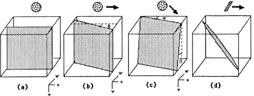
Fig

1a shows a bar which moves to the

left

with

time.

In

x-y-t

space

it

forms a

volume slanted

in

the temporal axis and the degree

of

slant corresponds to the velocity

of

the

bar.

The

task

of

motion

detection

could thus be viewed as

a

problem

of

detecting

spatiotemporal orientation.

f'

(a)

(b)

Fig.

I

- Image motion represented as spatiotemporal orienration in 3-dimensional x-y-t space

2.2

Motlon

ln

the

Frequency Domaln

Spatiotemporal

orientation

has a simple representation

in

the

frequency domain

fwatson &

Ahumada '851. Taking the Fourier transform of equation (1) gives :

Ff

<X-rxt,

y-ryt,

t)

=

F(u,v,

w+rxu+rrv)

(2)

Each temporal frequency is shifted by the amount - (r^ u +

r,

v), proportional to the local image

velociw.

[image:5.595.115.457.395.525.2]

-Fig. 2a

shows the specffum

of

a stationary pattern, where energy

is

concentrated

in

the uv-plane.

As

the pattern translates (Fig. 2b), the spectrum tilts into the temporal axis (w-axis), the

larger the

angle

0,

the larger

the

velocity.

Fig.

2c

illustrates the case

when

there are both

horizontal

and vertical

velocity

components, where the

horizontal

component

rx

is given by

tan

(cr)

and

the

vertical

component

r,

is

given

by

tan(F).

Finally, Fig. 2d

illustrates

the

spectrum

of

a

moving

edge. The edge, being one dimensional, produces a one dimensional

spectrum which is concentrated about a line through the origin. The plane cannot be determined

unambiguously, hence

only

the velocity component ofihogonal to the edge can be found. This

is commonly termed the apernrre problem [Marr & Ullman'81).

@+

@1

(c)

(b)

w

u

(

w

u

(

_(d)

Fig.2 - Representation of motion in ttre frequency domain (see tcxt).

3.

Extracttng

Irnage

Motlon

For the

purposes

of

deriving

an

optical

flow field,

we require

only

the

local

uanslational

information. This is

because non-rigid motions, rotation and scaling produce a varying two

dimensional

flow field

except

at

relatively small

image

regions.

By

taking

a

small

spatioremporal

window at

each

of

these image regions and

fitting

a

plane to

each

of

their

frequency spectra, we can estimate the true velocity

flow

field of the image sequence.

3.1

Spatlotemporal

d.entatlon

Deteetlon

There

have been several

methds

proposed

for

extracting spatiotemporal orientation from a

sequence of images. One rnethod is the use of spatiotemporal

filters

lLleeger 871. Heeger used a

family

of

Gabor-energy

filters

that were tuned to different spatial orientations and temporal frequencies.

By

combining the responses

of

each

of

these

filters

in

a least square manner and

normalising the response

from

each spatial orientation separately, he was able to resolve the

aperture problem and extract the unambiguous velocity

for

a great

variety

of

highly

textured

fanslating

patterns.

[image:6.595.87.527.248.414.2]

Bigun and Granlund proposed a rnethod

fordeternining

local orientation in a multidimensional space.

Their approach is

analogous to the probleru

of

reducing three dinrensiclltal tensors to

their

principal

axes,

but

applied to the spectral energy

in

the Fourier domain IBigun & Granlund

'87),

As

shown

earlier

in

Fig.

2d, the

spectral

energy

of

a

linearly moving

edge

is

always

concentrated

on

a

line

through the

origin

in

the

Fourier

dornain.

If

we consider the spectral energy as masses rotating about the axis ko, then the inertia about the axis

ko

is given

by

:

I(kp)

= I

F(k)

12

ot

where

d(k,kp)

is

the Euclidean distance function between each

position in

the Fourier space

and

the

line

represented

by

the axis

ko. (To simplify

expressions, the

x-y-t

space

will

be

represented by the vector x and the u-v-w frequency space

will

be represented by the vector k).

The problem here is to

find

the axis ko that minimises the inertia function

l(kp).

This could be

solved by formulating an eigenvalue problem given by

(3)

oo

l's

j

d'(k,kp)

-6

I(kp)=

kotJto

(4)

(s)

where

lkpl

=

I

and is orthogonal.

J

is the inertja tensor

matrix in

(3) whose diagonal elements

are

Jii

=

j*i

oo

f^a

J

k:'

I

F(k)

l'

dk

-6

and

non-diagonal elements are

Jij -

_J

*,

k;

_I

F(k)

12

dk

Finding

the

minimum inertia I(kp),

corresponds to

energy

in

the least squared error sense' This is given

of

J.

finding

the axis

ko

that

fits

the spectral

It

is possible to solve this eigenvalue problem in the spatial domain.

Utilising

the differentiation propefiies

of

the Fouries transfonn , it can be shown that fBracewell '861 :

r,2

_In{r)

t2 =

-#

,fr,t

and

k;k;

_rF(k)t2

=-#,frfr,

(7)

With

(7)

and

Parseval's theorem, we can ffansform the integral in equations (5)

&

(6) from the

Fourier k-space to the spatial x-space using the inverse Fourier transform.

Furthermore,

to

limit

the determination

of

image

velocity to

a

locality

at image

point

xo, a

weighting

fun*ion

g(x)

is utilised to control the size

of

the effective neighbourhood The final

expression

for

the diagonal elements of the inertia tensor matrix are

J11

(xs)

₌

I

(8)

j*i

;

.6r.r

;

g(x-x6)

(. )'dx

J

OXj

The inertia tensor matrix J could be expressed in another form :

J=

f

trace(A)-A

and for non-diagonal elements :

oo

(

r..

/v

_,)

_{= _ |}

g(x_xs)

(

"rJ

r^o,

J

".

-oo

€

A;1

(xe)

=

_f

_91*-*o)

(5)t

o*

I

dxi

and non-diagonal elements:

(

_,6f

Df,

A1i

(xs)

=

J

s(x-xo)

(.*,

Un,

o*

*fr".

(e)

(10)

where the trace

of matrix

A

is the sum of its diagonal elernents and

A

has diagonal elements :

(11)

(r2)

lt

can be

shown

that both the J and

A

matrices share the same eigenvectors lBigun and Granlutd

Finding the eigenvector corresponding to the least eigenvalue

J

is now equivalent to hnding the

eigenvector corresponding

to

the largest eigenvalue

of

A.

There

are several advantages in

dealing

with matrix A

instead of J and this

will

be become apparent

in section 4.

The elements

of

A

associated

with

the neighbourhood

of

the image

point

xo

can be evaluated

by

simple

summation

of all

the partial

derivatives

within

the

weighted

neighbourhood. These partial

derivatives being

first

obtained through appropriate partial derivative f,rlters.

In this work,

the weighting window g(xo)

was a

5x5x5 Hamming window

and the partial

derivative

filters

were designed utilising the 3x3 edge detection kernel of Wilson and

Bhaleroa-fWilson & Bhaleroa'90). The eigenvalues and eigenvectors

of matrix

A

were evaluated using the

NAG library

routine FO2ABF

for

a symmetric matrix. This routine reduces the marrix to upper Hessenberg

form atrd

uses _{the QR} algorithm to determine all eigenvalues and eigenvectors.

3.2

Interprettng the

elgenvalues

and elgenvectorg

The solution to the eigenvalue problem of matrix

A

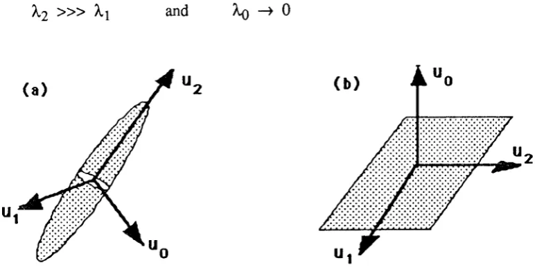
yields 3 positive eigenvalues :

)'z'7l

>

_h

>

0

(indescendingorder)

and their corresponding eigenvectors u2,

ut,

u6. When the grey-levels in the image sequence

are constant, we have :

ltZ=7\=h=0

(1 ₃₎

Under these

conditions,

no

velocity

vectors are obtained.

In

image regions where

there

are

moving one dimensional features like lines and edges, the spectrum is concentrated about a line

through the

origin

given by the eigenvector u2r corresponding to the iargest eigenvalue

Iz

(see

Fig. 3a). Under these conditions :

)rZ

,>, )"t

and

IO

_-

0 (14)

Fig. 3 - Eigenvectors corresponding

n

(a) a translating edge and (b) a translating _!-D pattern

[image:9.595.118.506.543.739.2]

In

regions containing moving two dimensional features

like

corners and textured surfaces, the spectrum

will

be concentrated about a plane through the

origin,

the normal to which is given by

the

eigenvector u0,

corresponding

to

the

least eigenvalue L9 (see

Fig.

3b). Under

these

conditions :

)tZ'

)tt

and

lo-0

Using

simple

vector

geometry,

it

can

be shown that the horizontal

and

vertical velocity

components

in

the direction of the image gradient are given

by

:

(1s)

rr

_Yx

_{= ---)}

ux ut

t

ux- +

uy-

and

Vy=

-

o*2

*

ur2

(16)

where ux, uy, ur are the components of the eigenvector u2.

This

velocity

cannot, under most circumstances, be regarded as the true image

velocity.

The

true image

velociry

can only be extracted when the spectrum

fits

unambiguously about a plane

and this

velocity

is given by :

v*=

ux

ut

u

and

Vv

_'ur

= (17)

where u1, uy, u1 &re the components of the eigenvector ug.

Another

useful

ffteasure that can be extracted

from

the three eigenvalues

)rz,Lt

and l,g

is

a

realibility

measure

of

the estimated

velocity

at each image point. This certainty value C(xg ),

indicates

how

well

the frequency spectrum

fits

a

line or

plane

in

a least squared

elror

sense,

and is given

by

:

C(xs)

₌

I ( 18)

1,9+l,t+7"2

The certainty measure C(xo ) is normalised and thus takes a value between 0 and 1; the closer

the value is

to

1, the more reliable is the velocity estimate.

4.

Cooperatlve

boundary detectlon

and

veloelty

freld smoothlng

Studies

of

the human motion detection system fVan Doorn & Koenderint 831 suggest that high

noise

immunity

is

achieved through spatiotemporal

integration

of

motion

information

over

extensive spatial area and time duration. However, this integration process does not

blur

out

the

visibility

of

boundaries demarcating regions moving

with

different velocities. This implies

that spatiotemporal integration

of

motion

information is in

some way guided by constraints

such as the presence of motion discontinuities.

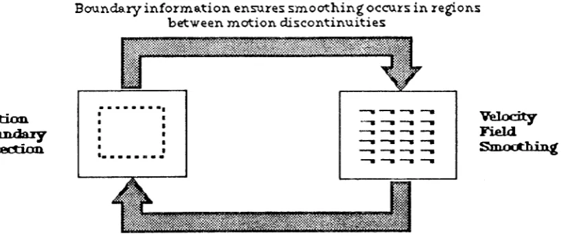
Boundary

information

en$res

sm o othin g oc(alrs

in re$ons

between

motion

discontinuities

Itotim

BGDdsry

Dceci@

Rtocity

fi€td

Sn€ctbing

Smoothed

velocity field

improves rnotion

boundery

detection

Fig. 4 - Cooperative interaction between motion boundary detcction and velocity smoothing

A

scheme is proposed here, as shown

in

Fig. 4, where both the detection of motion boundaries

and the spatial integration

of

local

velocity

estimates occur

in

tandem. Each process interacts

with

the other

in

a manner that serves to improve both the detection

of

the motion boundaries and the smoothness of the velocity

flow

field.

4,1

Veloctty

field

smoothlng

This

algorithm

achieves velocity

field

smoothing

in

an iterative manner, propagating

velocity

information from each image

locality

to its spatial neighbourhood. The propagation of velocity

information is

weighted

by

its

certainty

measure, ensuring

the

suppression

of

poor

initial

velocity estimates and enhancing the influence of more reliable ones.

[image:11.595.102.516.254.426.2]

As

shown

earlier in

equations (11)

&

(12), the

nratrix

A

at

point

xo is obtained

by

sunrnring

all

partial derivatives

within

its windowed neighbourhood.

In

order to achieve more extensive

iltegration

of

ntotion information, this summation is extended to include the partial derivatives

of

the

A

ntrtrices frorn

the

8

image

points

immediately

surrounding

point xo.

At

the kth

iteration, the summed elements of the

A

matrix at image point (xo, yo) is given by :

A11 (xo,y6 ;

k) =

^t

,

i

F'(xo+n,yo+m

;

k-1)

A11 (xo+n,yo+m _; k-1) (1e)

The

certainty

measure C(xo+n,

yo*m

; k- I _{) for} each

of

the

A

matrices in the neighbourhood is

defined

by

equation

(18). Its

value

is

squared

to

increase the suppression

of

poor

velociry

estintates.

After

surnmation

of all

the neighbouring

A

matrices, each matrix element

of

the

resulting

A

rnatrix is nonnalised appropriately as shown :

A1i (xo,

ye;

k)

₌

Ail

(xo, yo

;

k)

(20)

j i

"'(xo+n,

yo*m;

k-1)

n=-l

m=-l

With

each successive iteration, the spatial extent

of

motion information integration is enlarged

This occurs

because

local velocity

estimates

are being

progressively passed

from

one

neighbourhood to another through the iterative neighbourhood summation process.

With

the

use

of

a

certainty

weighting function C(xo), the integration process enhances the propagation of good

inirial

velociry estirnates while suppressing the effects

of

unreliable ones.

Some

of

the

results of the velocity smoothing algorithm are illustrated below. Fig. 5 shows the

centre frame

of

the

image

sequence used.

The

sequence

is

corrupted

with

additive

spatiotemporal Caussian

white

noise and has a

signal-tonoise ratio

of

l0dB.

(a)

(b)

[image:12.595.84.516.533.725.2]

The

first

sequence has the

circle

shown

in Fig.

5b nroving

linearly with

a

velocity

of

0.5

pixeVfranre. The velocity estimates illustrated

in

the examples below are all taken from level I

of

the sparial lowpass pyrarnid

of

each frame

in

_{the inrage sequence lBurt&Adelson} 831.

Fig.6

show,s the

effect

of

the snroothing algorithm at

various

iterations. Good

initial

estimates are

obtained

in

areas

with

a

strong

intensity gradient,

such as the edges

of

the

circle,

and are

progressively

propagated

inwards

and outwards.

By

a combination

of

the propagation

of

strong

motion

energy at the

circle

edge and the suppression

of

poor

velocity

estimates, the

random noise

in

the

vicinity of

the circle appears to move

in

a coherent

fashion,

in a similar

way to

that

of

the circle.

This

phenomena called

motion

capture fRamachandran

&

Anstis 831 is observed by the human visual system.

(a)

(b)

(c)

Fig. 6 - Velocity field of circle moving rightwards. (a),O),(c) are results at iterations I,5&20 respectively.

This

smoothing

dgorithm

is

effective

not

only

for

translational motion.

As

shown below in

Fig. 7,

the radius

of

the

circle is

now expanding at 0.5 pixeVframe. As most natural velocity

flow fields

are smoothly

varying,

except at

motion discontinuities, this

algorithm is able to

integrate neighbouring velocity estimates to produce

a

smooth velociry f,reld.

(a)

(b)

Fig.1 - Velocity field of expanding circle. (a),O),(c) are resulr at iterations l, 5 & 20 respecrively.

!ill

lnirll'

f:;i

.ltl

::::

[image:13.595.79.545.247.422.2] [image:13.595.81.547.555.735.2]

To avoid

integration

of

motion information

across

motion

discontinuities, image points that have been identified as boundary points by the motion boundary detection algorithm in section

4.3,

ate not considered

in

the neighbourhood summation process. In other words,

if

an image

point

xo

is

sunounded

by

8 neighbouring points,

of

which

3 are boundary points. Then the

summarion process

in

equation

(19)

will

only involve

the other

5

good neighbours and the

resultant A

matrix

will

be normalised accordingly.

4.2

Netghbourhood

summatlotr

at

boundary

polnts

If

an

image

point

xo

is

a

boundary

point,

it

will

not

undergo

the certainty

weighted

neighbourhood summation described

in

equation

(19).

Instead,

all its

8 neighbours

will

be

summed

with

equal weighting irregardless

of

whether they are boundary points or points

with

good velocity estimates. The elements of the A matrix

of

a boundary point at the kth iteration is

then :

1lt

Aii

(xo,ys;

k)

=

g

^?,,J_rotj

(xo+n,yo+m;k-1)

(21)

If

a boundary point actually lies on a motion discontinuiry, the equal weighted summation

of

its neighbourhood

will

ensure its certainty measue remains poor throughout the iterative process, thus maintaining a barrier which

will

prevent motion information of different velocity regions

from

intermingling.

In

cases where the boundary

points

are detected

falsely

due

to

the presence

of

noise, this

summation

of

the neighbourhood

will

progressively improve its certainty measure, eventually

4.3

Motlon boundary

detectlon

The

motion

boundary detection

algorithm

was inspired by the n-rodels proposed by Reichardt

and Poggio from their studies

of

relative motion discrimination abilities

in flies

lReichardt and

poggio '791.

-I\ey

suggested

that

large

field

pool cells sum information

from

many small

field

motion detector cells and

it

is this summation

of

motion detectors over an extensive spatial area

that allows

the large

field

cells to

detect the presence

of

motion

discontinuities

within

that spatial extent.

A

similar summation scheme is used here.

The detection

of

boundaries between

two

regions of

differing

velocities relies on the fact that

the certainty

measure at these image

locations

is

generally much poorer than

in

areas

with

smoothly varying

velocity

fields.

By

summing

over

a

large spatial

area

at

motion

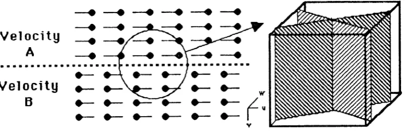
discontinuities, we would obtain a frequency spectra similar to that shown in

Fig.

8. Since the

spectral energy is concenffated in two different planes, attempting a least square error

fit

of this spectra into a single plane

will

result

in

large errors. This is shown up

in

the eigenvalues of the

matrix

A.

Eigenvalues 1"2, 1,1 and 1,g

will

all

be much greater than

0, resulting

in

a low

certainty measure.

-a

--a

Vel

oci

tg

__{

---a

_-{

l-Vel oci

tg

o-B

;-Fig. 8 - The frequency spectra at a motion discontinuity contains spectral energy ftat is concentrated about two

Jiff"r.nt planei corresponding to two distinct velocity regions. Poor certainty measures are obtained in this

region because an opdmal plane fit results in large errors.

Similar

neighbourhood summation of

A

matrices as in equation (19) is used here, except over a

larger

spatial

neighbourhood.

In

our

implementation,

an 8x8

neighbourhood was

used.

Another

variance from equation (19)

is

the normalisation

of

each element

of

matrix

A

by

the

total

sum of all

is

elements. This reduces the bias in the frequency specfra that may arise due to

a non-uniform intensity gradient

within

the neighbourhood'

A

circular

window

function is

used to reduce the influence

of

regions that are further away

from

the centre.

-{

--a

o-

O-

o--o--

o-o- O-

u/

O- O- ,/

;-

>-

r'

[image:15.595.95.503.394.531.2]

'fhe

_{ele rlcnts of the sumrned matrix}

_A

_{at point (xo, yo) on the kth}

_iteration

_{is given by} :

A11 (xs, ye

;

k)

=

1!11l!1".",

v"..

;

k-lt

*ftO

N4(xo+n, yo*m ; k-1)

where the normalising

factor

:

N6(xo+n,

yo*rlt

; k-1)

lAli

(xo+n,

yo*m

;

k-1)

I

and the rvindorving function :

44

IT

n=-4 m=4

(22)

(23)

(24)

133

=oI t

' i=l

j=l

w(n,m)

₌

6.66 {/ .

t'?

After

neighbourhood summation

of A

marrices

for

every image

point, their

corresponding eigenvalues are evaluated and their cerrainty nleasure

C(xd

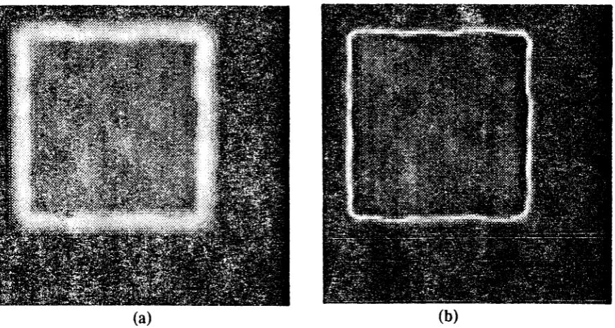
found using equation (18). Fig. 9a

shows a scaled

plot of

the certainty measure

for

a random dot image sequence. As a result

of

surrrmating

over

a large neighbourhood, the motion boundary is

fairly

wide. [n order to detect

the motion

boundaries

more precisely, boundary thinning

must

flrst

be performed

on

the

certainty image in Fig. 9a.

Fig. 9 - A noise free random dot image of a moving square. (a) shows a linearly scaled plot of is certainty

[image:16.595.86.531.472.709.2]

Boundary

thinning

is done

in

the

following

nranner. Firstly the gradient,

C'(xo)

at each point

of

the certainty image

C(xd

is obtained :

C(xo)

=

The boundary image is then obtained

from

the expression :

B(xo)

₌

C(xo)

(

C'(xs)max

-

C'(xq)

)2

ru{}r'.

tDSi'

(2s)

(26)

where C'(xs)rneu( is the largest gradient

value

in

the certainty image and

is

used to scale the

boundary image B(xo).

Boundary points are selected by setting a threshold value on the scaled boundary image B(xo).

The selection

of

a suitable threshold value

is

not too

cirtical.

If

the threshold

is

set too high,

q'eak

_motion

boundaries

may

not

be

detected and 'leakage'

may occur

between

different

nrorion regions.

When

neighbourhood

summation is

done

in

these

regions, the

resulting

certainty measure

of

the summed

A

matrix

will

deteriorate (see Fig. 8). This progressive drop

in the certainty value

will

eventually

'plug

up' the leak. This is a benefrt

of

the adaptive nature

of

the

velocity

smoothing

algorithm;

as the certainty measure at the

kth

iteration

is

obtained

from

the neighbourhood summed

A

matrix

generated during the

(k-1)th iteration.

However,

the resulring motion boundary

will

be

slightly

biased towards the region rvhich had a poorer

inirial

certainty

measure.

An

effective

technique

to

prevent leakage

is to

start

with

a low

threshold value and progressively raise this threshold with each iteration.

The

position

of

boundary

points found

by this

algorithm

is

fed

back

to

the

velocity field

smoothing algorithm. l,ocations

of

new boundary

poins

are updated before proceeding to the

next iteration

of

snloothing. Likewise,

boundary points that have

fallen below

the

new threshold value

would

revert back to points having good velocity estimates.

5.

Experlmental

Results

All

results presented

in

this

section

were

computed using

the

lowest

level

of

the

spatial

lowpass pyramid.

Additive

spariotemporal Gaussian white noise was added

to

all

test image

sequences to obtain a signal-to-noise

ratio

(SN,R)

of

i0dB. The SNR is

defined by

:

;r

where

o;2

and

on2

are the

variances

of

the

clean image

sequence

and

added

noise respectiVely.

5.1

Translatlonal flow

field

A

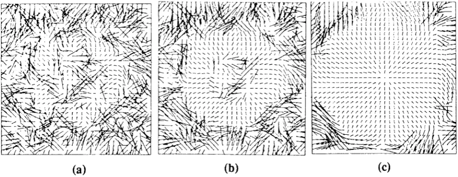
square was extracted from a static random dot image and made to translate

diagonally with

each consecutive

image frame. The moving

square's

horizontal and

vertical velocity

contponents were both 0.5 pixeVframe. The velocity

flow

fields are shown below in

Fig.

10.

(a)

(b)

(d)

Fig.

l0

- Moving random dot square. Each vector in the flow field is depicted by a line whose length and

direction is proportional to the velocity estimated at that image point. (a) I frame from the image se.quence with

a SNR of t0OS. (b),(c)&(d) Velocity flow field at iterations 1,5 and I

l

respectively. The boundary points seen

as light grey dots reveal the slructure of the moving square patch. False boundary points at image regions badly affected by noise are progressively removed with each itcration.

r r'ii

\\'

\\'

\\'

\\:

\\;

\\:

\\t'

\\

\ \11

\ \ii \\i '_-!'

\\\\\\\\\\\

\\\\\\\\\\\

\\\\\\\\\\\

\..

\\\\\\\\

\

\

\,

\\\\\\\\\

\\\\\\\\\\\

\ \\\\\\\\\

\\\\\\\;

\\\

\\\\ \\\\\\\

\\\\\\\\\\\

\\\\,\\\\\\\

\\\\'-\\\\\\

\\\\\\\\\\\

\\\\\\\\\\\

;'\\\\\\\\\\

\\\

\

\\\\\\\

\\\\\\\\\\

_{\\\\ \\\ \\\ \}

\

\ \ \._\.\.\._\.:.\.\ _^\ \

\.\.\'

\

\\':: \\

\\\\\ \

\.

\\\\\

),,\\.\.\.\.

'"

.:::::.--=:

\\\\\\\\\\\\\rrrrr$

\\ \\\\\\\\\\\

\

\

\\\\:'

\\\\ \ \\ \ \ \\\\ \\\\ \]i'

\

\\\\

\ \ \ \ r

rr\.

r r r \' _{r $.'}

\\\\\\\\\\\\\\\\\\X'

_{\\\\\\\\\\\\\\\\\\\'}

\\\\\ \\\\ \\\\\\\\

\ \_:

\\\\\\\\\\\\\\\\\\\:

\ \ \\\ \\\\ \ \\ \ \ \\\ \ \ji

\\\\\\\\\\\\\\\\\\\i

\\\\\\\\

\\\\\\\\\\v

\ \

\\\\\\\\

\\

\ \

\\\

\ \j'

\\\\\\\\\

\

\\\

\\\\\v

\

\\\\\\\\

\\\\ \\\\ \i'

\

\\\\\\\\\\\\

\

\\\\\-\\\\\\\\\\\\\\\\\\\i

\ \ \\\\\\\\\\\ \ \ \ \ \ \i

\\\\\\\\\\\\\\rrrrf

[image:18.595.89.551.202.668.2]

At

the 1Oth iteration, the nrean horizontal and vertical velocity components

rvithin

the ntoving

square

patch were

estimated

at

0.534 pixel/frame

(V^)

and 0.538 pixeVframe (Vr)

respectively.

Their

respective variances were 0.0004 and 0.0004. The ntean percentage error

esrimated

for

V*

was

6.9Vo

and

7.17o

for

Vr.

This

accuracy

is

comparable

to

the

results

obtained

by

Heeger flteeger'87).

The boundary images for the same

moving

random dot square at various smoothing stages a-re

shown

below.

The position

of

the

motion

boundary has a tendency to be biased towards the side

of

the region wirh poorer

initial

certainty measure, they are usually areas

with

a weaker

Fig. I

I

- Boundary images of the moving random dot _{square $Querrce. (a) shows the estimated} molion boundary

orlerlaid over tie actual motion boundary of the centre image frame. (b),(c)&(d) are boundary images at iterations

l,

5

&

I

I

respectively. Observe how the weak motion boundaries (eg: top left edge, just below t}re corner) were

progressively reinforced wirh each iteration. Regions within the moving square patch that were significantly

conupted by added noise were gndually smoothed oul

intensity gradienr

[image:19.595.86.553.235.685.2]

5.2

Rotatlonal

flow

fleld

A

rorarional

velocity

flow field

was generated

by

applying

rotational

transforntation

to

the

ranclom dots

u,ithin

a circle

of

radius

50

pixels, centred at the ntiddle

of

a static randont dot inrage. This rotation has an angular

velocity

of

1 deg/frame. The rotational

velocity

flow

field

obtained

by

application

of

the cooperative boundary detection and

velocity

field

smoothing

algorithm

is shown below in

Fig.

12.

Fig. 12

-

Rotating random dot circle with SNR

of l0dB. (a)

Shows one frame from the sequence- The

ro6tional transforiration was done on an image twice the size and was then spatially lowpass subsampled to die required size for generating the roradng sequence. This was Lo reduce ermrs caused by the discrete nature of

the transformation a-igorithm. (u),(c)a(d) Srrows rhe rorational velocity flow field at iterations 1,5 and 20 respectively.

(b)

[image:20.595.85.556.189.644.2]

Error estirnates

for

the rotational

velocity field

were obtained at the 15th iteration. The ntean

percentage

error for

the

velocity

components

V^

and

V,

were 12.87o and 15.07a respectively

(only

non-boundary points and points

with velocity

components exceeding 0.01 pixeVframe

r,r'ere conside red in evaluating the nlean percentage error).

The boundary images

for

the same rotating random dot circle at various smoothing stages are

shown below.

Fig. l3 - Boundary images of rorating random dot sequencel (g) _1n9ys the estimated motion boundary overla.id

on"the actual *otion uounoary of thE centre image frame.(b),(c)&(d) are boundary images at iterarions

l,

5 &

20, respectively.

18

-'i

7 I

{

;/

I

T'

t:

i1 l: I

I

I

[image:21.595.87.551.201.656.2]

6.

Summary

This

report

has described

a

technique

for deriving

the

optical

flow field

in

noisy

image sequences

which

contain motion discontinuiries.

It

has been shown how

local

image nrotion can be characterised as spatiotemporal orientation, and this orientation can be detected

in

the

spatiotemporal frequency

domain

as spectral energy concentrated about

a plane

or

a line

through the

origin.

A

technique analogous to an eigenvalue analysis

of

the

inertia

tensor was

used to determine this orientation.

This

technique was

further

extended

to

smooth

velocity

flow

fields

by

integrating

motion

information at each

locality with

that

of

its immediate neighbourhood.

An

iterative algorithm

was developed that

ensured

this

smoothing

was constrained

by

the detection

of

motion

discontinuities.

A

further

strength

of

this algorithm

is its ability to

propagate

good

initial

velocity

esrimares

while

suppressing unreliable ones.

This

has the

effect

of

improving

the

overall accuracy of the optical

flow

field

obtained, even under

fairly

noisy conditions.

The cooperative motion boundary detection and velociry

field

smoothing algorithm was shown to

perform well

on both translational and rotational random dot image sequences. The mean

percentage error

of

the

velocity

estimates for translational motion was less that 87o, which is

comparable

to

existing motion

estimation techniques applied

to

similar noisy

random dot

sequences moving at subpixel velocities flleeger'871.

The present

work

described here has only taken into account the spatial integration

of

motion

information. Further improvement

in

noise immunity could be attained through the combined

spatial and temporal integration of motion information. There is also a need to combine in some

meaningful way, the

velocity

estimates at various levels

of

the lowpass spatial pyramid. This

will

enable the detection

of

a greater range

of

velocities

within

the image sequence without

unduly sacrificing the detection resolution of motion boundaries at regions

moving

with

slower

7.

References

IEH

Adelson

&

JR

Bergen'S5]

-

"Spatiotemporal energy__models

for

the

perception

of

motion",

J. Opt. Soc.

Am

A/Vol

2, No.2, Feb '85, pp 284-299.

IJK Aggarwal

&

N

Nandhakumar '881-

']On_

computation

of

motion from

sequences

of

imagei-

a

review",

Proc.

of

IEEE

Vol.76, No. 8

Aug

'88 ,pp 917-935.

IO

Braddick'74

]

-

"A

short range process

in

apparent

motion", Vision

Res.

14,

pp

519-527.

IJ

Bigun

&

GH

Granlund'87] - "aptimal

orientation detection

of

linear

symmetry",

Proc

of

IEEE

ICCV

,

Jun'87,

pp

433-438.

IJ

Bigun

&

GH Granlund SS]

-

"Optical

flow

based

on

the inertia

matrix

of

the frequency

domain",

Proc

of

SSAB on Image processing,

Mar'88.

IRN

Bracewell'86

]

-

"The Fourier transform and its

application",

McGraw

Hill

books.

IPI

Burt

&

EH

Adelson'83

I -

"The Laplacian

pyramid

as a compact image

code",

IEEE Trans.

COM,

Apr'83,

pp 532-540.

IDJ Heeger

'8n

- "Optical

flow

using spatiotemporal

filters",

J. Opt. Soc.

Am

A/Vol

4, No.8,

Aug

'87,

pp

1454-1471.

1BKP

Horn &

BG

Schunck'8Il -

"Determining optical

flow",

AI, Vol.

17

Aug

'81,

pp

185-203.

lD

Marr &

S

Ullman'81)

-

"Direcfional

selectivity and

its

use

in

early visual

processing", Proc.

R.

Soc.

Lond.

B

2i1

'81,

pp

151-180.

IVS Ramachandran

&

SM

Anstis

8fl

-

"The perception

of

apparent

motion",

Sci.

Am.

Jun

'86,

pp

80-87.

IW

Reichardt

&

T

Poggio '79)

-

"Figure-ground

discrimln1iign

by

relative

movement

in

the

visual system

of

the

fly",

Bio.

Cyber.

Vol.

35,'J9,pp

81-100.

IAJ VanDoorn & JJ

Koenderink'83)

- "The structure

of

the human motion detection system",

ipEE

Trans.

SMC

13,

No. 5, Sep'83, pp918-922

IAB

Watson

&

AJ

Ahumada

S5l -

"Model

of

human

visual motion

sensing",

J.

Opt.

Soc.

Am

A/Vol

2, No.2, Feb '85,

pp

322-341.

IRG Wilson

&

A

Bhalerao '90f

-

"Kernel 49rig.n

for efficient multiresolution

edge detection

and orientation

estimation",

July 90, in publication, IEEE Trans.

PAMI.