Three phase integrated load and harmonic flows

(1)

A thesis presented for the degree of

Doctor of Philosophy in Electrical and Electronic Engineering in the University of Canterbury, Christchurch, New Zealand.

(2)

(3)

ABSTRACT

This thesis investigates two algorithms for the steady state analysis of HVDe convertor plant.

The first is an already well established frequency domain technique, known as IlIA (Iterative Harmonic Analysis), and the investigation centres on the nature of the al-gorithm under divergent conditions. In particular, a mathematical analysis of the algorithm is used to prove that divergence of the algorithm is not necessarily indicative of a physical harmonic instability.

The second algorithm is developed to exploit the IHA technique within the context of the three phase a.c.-d.c. loadflow as an alternative convertor model which incorpo-rates (rather than ignores) the effects of harmonics. The resulting three phase inte-grated load and harmonic flow algorithm is a significant improvement on the existing single phase load & harmonic flow algorithms.

(4)

(5)

CHAPTER 3 INSTABILITY IN ITERATIVE HARMONIC ANALYSIS

3.1 Introduction

3.1.1 Review ofIHA Research 3.2 Uncharacteristic Harmonic Production

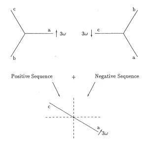
3.2.1 Nature of the triplen harmonics produced 3.3 Mechanisms of harmonic magnification

3.3.1 Phase Angle Control 3.3.2 Equidistant Firing Control

(6)

3.3.3 The Representation of 'Dynamics' 3.3.4 Numerical Noise

3.4 Divergence Unrelated to Uncharacteristic Harmonics 3.5 Analysis of IHA

3.5.1 Gauss-Seidel Nature of IHA

3.5.2 Multivariable Convergence Constraint 3.5.3 Application to the Convertor

3.5.4 A case with filters

3.5.5 Interpretation in terms of continuation methods 3.6 Conclusions

38 41 44 47 47 49 49 54 56 57 CHAPTER 4 INTEGRATED LOAD AND HARMONIC FLOWS 59

4.1 Introduction 59

4.2 Three Phase Integrated Load and Harmonic Flows 62 4.2.1 The Three Phase A.C.-D.C. Load Flow 62 4.2.2 Integration Of The Two Algorithms 66 4.2.2.1 Fundamental Power Flow 66 4.2.2.2 Harmonic Power Flow

4.2.2.3 DC system consistency. 4.2.2.4 Zero Crossing Control 4.2.3 Form of the combined solution. 4.2.4 Convergence Considerations 4.3 Initial Test Results

4.3.1 Unfiltered Case 4.3.2 Shunt Capacitor Case 4.3.3 Filtered Case

4.4 Conclusions.

CHAPTER 5 PRACTICAL APPLICATIONS 5.1 Introduction

5.2 Tiwai Aluminium Smelter 5.2.1 Unfiltered Case 5.2.2 Filtered Case

5.3 Harmonic Interaction Between Benmore and Tiwai 5.3.1 Effect of Remote Harmonic Injections

5.3.1.1 Globally Characteristic Harmonics

68 69 73 74 75 75 76 76 77 77 79 79 79 82 85 88 88 90 5.3.1.2 Locally Characteristic Harmonics 91 5.3.1.3 Globally Uncharacteristic Harmonics 91

5.3.1.4 Summary 92

5.3.2 Effect of Varying the Tiwai Delay Angle 92 5.3.3 Improving the Efficiency of the Algorithm 94 5.3.3.1 One 6-pulse convertor at Tiwai 96 5.3.3.2 6-pulse convertors at Tiwai and Benmore 97 5.3.3.3 One 6-pulse convertor at Tiwai, four at Benmore 97

5.3.3.4 Conclusions 98

(7)

5.4 Conclusions

CHAPTER 6 CONCLUSIONS

6.1 Discussion

6.2 Future Work

REFERENCES

(8)

(9)

LIST OF FIGURES

1.1 Capacitor and Inductor models in EMTP jEMTDC . 3

1.2 Structure of IRA algorithm 5

2.1 The basic Graetz bridge. . . 8 2.2 Equivalent circuit of the commutation process. 8 2.3 One cycle of rectification. . . 11 2.4 Separation of the transformer into (ideal) winding configuration plus

leakage . . . 12 2.5 Star-Star transformer winding configuration. 12 2.6 Star-Delta transformer winding configuration. 13 2.7' Calculation of D.C. voltage during commutation. 16 2.8 Flowchart of the IRA process applied to the convertor. . 18 2.9 Example of convertor interconnection. . . 19 2.10 A simple test system.. . . 22 2.11 Reconstructed waveforms from the IRA results of the simple test system. 23 3.1 Third harmonic content in the idealised phase current waveform. 28 3.2 System for deriving typical third harmonic generation. . . 30 3.3 Third harmonic current generated by unbalanced commutations. 30 3.4 Third harmonic current sequences. . . 31 3.5 Third harmonic components with a star-star transformer. . 35 3.6 Third harmonic current flow in a star-delta transformer. . . 36 3.7 Third harmonic components with a star-delta transformer. . 37 3.8 Iterations required for convergence with various <P3 & a star-delta

trans-former. . . . 38 3.9 Iterations required for convergence with various <P3 & a star-star

trans-former. . . . 39 3.10 Nature of zero crossing shifts due to characteristic harmonics.

3.11 Different sampling regimes for a balanced current waveform .. 3.12 Symmetric system including filters . . .

3.13 Effect of SCR on the convergence of IRA. 3.14 Analytically solvable test system . . . . . 3.15 Figure 3.14 redrawn for clarity. . . . . . .

3.16 Reconstructed waveforms after applying the BIRM technique. 3.17 Gauss-Seidel convergence and divergence patterns.

3.18 The three unique derivative functions.

3.19 Position of the inserted reactance pair. . . . .

40 42 44

44

45 45 47

48

(10)

4.1 4.2 4.3 4.4 4.5 4.6 4.7 4.8 4.9

Flowchart of the Q 'HARM algorithm. . . . . .

Convertor modelling within Q'HARM '" ..

61 62

Assumed convertor connection and waveforms. 64

Detailed flowchart of the three phase a.c.-d.c. loadflow. . 67

Decoupling between the convertor model and the real/reactive load flow. 68

Harmonic voltage and current relationships at the terminal busbar. 69

Simple loop configuration . . . 70

Position of the ideal tap-changing transformer. . . 71

Example of application of the tap ratio algorithm. 72

4.10 Selection of the reference zero crossing . . . . 73

74 75 4.11 Obvious form of the integrated algorithm . . . .

4.12 Integrated load and harmonic flow - initial test system ..

5.1 Tiwai seven bus system. . . 80

5.2 Filter arrangements at Tiwai. . . 82

5.3 Distribution of real power in the network. 85

5.4 Comparison of the a.c. systems used in the two conflicting filtered cases. 87

5.5 Interconnection of the South Island network for the harmonic interaction

study . . . , 89

5.6 Percentage changes in Benmore harmonic voltages with varying aTIWAI. 93

5.7 Efficiency improvement by reusing current phasors in IHA. 95

5.8 More efficient structure for the integrated algorithm. . . .

5.9 Variations in the 23rd & 25th harmonics with aBENMORE. . .

5.10 Variations in the triplen harmonics at Tiwai with aBENMORE.

(11)

LIST OF TABLES

2.1 A.C. current waveform sampling process.. . . 15 2.2 D.C. voltage sampling process. . . . 17 2.3 Comparison of Direct and IRA solutions for a simple case. 22 3.1 Commutating reactances governing each commutation. . . 29 3.2 Conduction period behaviour with a =200

• • • • • • • • • 33 3.3 Third harmonic levels with balanced current waveforms. (% of

funda-mental) . . . 43 3.4 Comparison of the first 5 characteristic harmonic currents 46 3.5 Inclusion scheme for BIRM. . . 46 3.6 Dimensions of the IRA-space for various cases. . . . 50 3.7 Dependence of phase currents on commutating voltages. 51 3.8 Convergence patterns with varying [J). . . 54 3.9 Terminal power flows at the original terminal busbar . . 56 4.1 Performance of the integrated algorithm without filters. 76 4.2 Performance of the integrated algorithm with capacitive reactive support. 76 4.3 Performance of the integrated algorithm with filters. 77 5.1 Physical component values in the Tiwai filters. . , . 81 5.2 Variations in fundamental frequency variables at Tiwai for the unfiltered

case. . . .. 83 5.3 Power in the convertor waveforms: with and without distortion. . . .. 84 5.4 Percentage changes in the unfiltered harmonics, with respect to the one

PQR case. . . 85 5.5 Variations in fundamental frequency variables in the filtered case . . . " 86 5.6 Phase two triplen increases for the filtered case. . . .. 87 5.7 Fundamental variable behaviour with and without remote harmonic

in-jections. . . .. 90 5.8 Perturbation to the 23rd _&₂₅th _{harmonics at Tiwai when the Benmore}

injections are introduced. . . .. 91 5.9 Effect of Tiwai harmonic injections on the Locally Characteristic

Har-monies at Benmore. . . . .

5.10 CPU savings with one convertor. . . . . . 5.11 CPU savings with two convertors. . . . . . 5.12 Current sampling processes with two convertors. 5.13 CPU savings with five convertors . . . .

91

(12)

(13)

LIST OF PRINCIPAL SYMBOLS

The following list of symbols is intended for guidance only, since all symbols are defined in the text. The flavour of some of the following symbols may vary slightly from chapter to chapter. Those symbols labelled as being 'generic' are used to refer to either the time domain waveform or the phasor representation, and mayor may not include distortion.

All functions of time may drop the

(t)

provided ambiguities are avoided.

aa, ab, a_{c -} off-nominal transformer tap ratios.

a - a constant vector.

bigO - a function which returns the largest element in its vector

argument.

b3 - third harmonic Fourier coefficient.

[C] - a connection matrix.

Cll C2 , C3 - zero crossings of the fundamental commutating voltages.

[D] - d.c. iteration Jacobian.

E - internal generator emf.

fO - non-linear function in the harmonic space.

t~

-

Jacobian of the non-linear function fO.

Eli I t f &f

aVj - e emen 0 aV'

gO - a general vector-valued function.

h - harmonic order.

ia(t), ib(t), ic(t) -

three phase current waveforms.

i~(t), i~(t), i~(t)

-

third harmonic current waveforms.

ibA (t), ibB(t), i1A(t) -

third harmonic branch currents in delta winding.

id(t) -

d.c. current waveform.

r(k) - kth iteration harmonic current vector. Id - d.c. current (generic).

(14)

i/i -

hth harmonic d.c. current component magnitudes.

IN - an harmonic Norton current source vector.

(J] - Jacobian of the IRA iterating function. la,

h,

le - commutating inductances.

lac, ha, leb - commutating loop inductances. Nc - number of convertors.

NT - number of terminal bus bars.

Nv - number of independent harmonic voltages.

N() - number of independent firing instants. Pd - d.c. side power.

Ph - hth harmonic power.

pu - per unit.

t - time.

Ts - sampling interval.

va(t), Vb(t), ve(t) - three phase voltage waveforms.

vae(t), Vba(t), Veb(t) - three commutating voltage waveforms.

v~(t), v?(t), v~(t) - third harmonic phase voltage waveforms.

v~e(t), v~a(t), V;b(t) - third harmonic commutating voltage waveforms.

Vd(t) - the d.c. voltage waveform.

v+(t), v-(t) - common-cathode and common-anode voltage waveforms.

V(k) - kth iteration harmonic voltage vector. Va, Vb, Ve - three phase voltages (generic).

Vah , Vbh , Veh - hth harmonic phase voltage magnitudes.

Va~, Vta,

vlb -

hth harmonic ccommutating voltage magnitudes.

Vae, Vba, Veb - three commutating voltages (generic). Vd - the d.c. voltage (generic).

Vh - an harmonic voltage (generic). VT, Vf - terminal busbar voltages (generic).

V+, V- - common-cathode and common-anode voltages (generic).

Vo - a constant harmonic voltage vector.

x(k) - a general kth iteration vector. Xa, Xb, Xe - commutating reactances. Xae , Xba, Xeb - commutating loop reactances.

Xc - commutating reactance.

(15)

[V] - harmonic space admittance matrix. [Y]h - hth harmonic admittance matrix.

ZCi - zth zero crossing of the commutating voltages.

Zh - an harmonic impedance (generic).

a - firing angle (generic).

ai - zth firing angle.

amin - minimum firing angle .

.6. - signifies a mismatch quantity.

e -

general angle (generic).

ei -

zth firing instant.

() - a vector of firing instants.

e -

a vector-valued function returning the latest firing

lll-stants.

fl - commutation overlap angle (generic).

fli - zth commutation overlap angle.

~i - convergence measure for phase i.

T - dummy variable of integration or continuation method

parameter.

1>~, 1>~, 1>~

-

phases of h th harmonic phase voltages.

1>~c'

1>ta,

1>~b

-

phases of hth harmonic commutating voltages.

1>h -

hth harmonic impedance phase.

(16)

/

LIST OF ABBREVIATIONS

BIRM - Binary Inclusion Relaxation Method. CPU - Central Processing Unit.

EMTDC - Electromagnetic Transients for DC. EMTP - Electromagnetic Transients Program.

FFT - Fast Fourier Transform. GCF - Greatest Common Factor.

HA - Harmonic Analysis Iteration. HVDC - High Voltage Direct Current. IHA - Iterative Harmonic Analysis. LHS - Left Hand Side.

MRFFT - Mixed Radix Fast Fourier Transform. NLR - Non Linear Resistor.

OLTC - On Load Tap Changer. PC - Personal Computer.

PQH - P Iteration, Q Iteration, Harmonic Iteration. RHS - Right Hand Side.

(17)

ACKNOWLEDGEMENTS

Completion of this thesis marks the end of a major portion of my life, and it would be unfair to let it pass without some acknowledgement of those people who have played a significant part in it.

Firstly, to my supervisor, Professor Jos Arrillaga, without whose gentle supervision this project would never have left the ground.

Secondly, to my colleagues whose friendship, support and advice helped lighten the long term effort. In particular I would like to single out Drs. Julian Eggleston, Neville

Watson, Enrique Acha & Ranil de Silva, and postgraduates Gordon Cameron, Aurelio

Medina, Sankar and Jerczy Ciechanowicz.

Thirdly, to my employers, Trans Power (NZ) Ltd., by whose generous study leave and financial support I am able to complete this thesis.

Thanks also to my parents, who have never wavered in their support and confidence in my abilities over ( especially) the past three years. They will, nonetheless, be relieved when it is all over.

I would like to make special mention of Dr. Richard Fright, who was a source of both friendship and inspiration not only to me, but to all who were associated with him.

(18)

(19)

CHAPTER 1

INTRODUCTION

1.1 HARMONIC SOURCES IN POWER SYSTEMS

To the casual observer the power system is often seen to be a bastion of certainty - an ideal source of single frequency power, neither deviating in magnitude, phase or frequency. The truth is rather different, however, and this has necessitated the development of power system analysis as it exists today.

Although, for many years, the purity of the power system waveform was held to be unquestionable, the current message is that power systems, as with almost all other systems, suffer from pollution - pollution in the form of harmonics.

In principle, any non-linear device is a potential source of waveform distortion, and the modern power system is full of examples. In spite of the linearity of transformer and generator models developed for, say, loadflow purposes, both of these fundamental power system elements are examples of non-linear devices, due to the non-linearity of the transformer magnetising characteristic, and the coupling between frequencies within the stator-rotor interactions in the generator.

However, the real culprits behind the wholesale harmonic pollution of the power system are the power electronic switches, whose presence permeates almost every aspect of the electricity industry: from generation, through transmission and distribution to consumption.

In New Zealand they are of particular importance given that nearly half of the South Island hydro resources are given over to supplying rectifier loads, while the North Island receives a significant proportion of its supply from the South Island via an HVDe interconnection. With planning underway to double the capacity of this link (and therefore the attendant harmonic generation) the associated harmonic phenomena can only increase.

1.2 HARMONIC ANALYSIS OF POWER SYSTEMS

Effective action to reduce the generation of harmonics, or to reduce in some way their detrimental effects may only be taken if the presence of harmonics can be predicted, and moreover quantitatively assessed during design stages. This is, however, only possible if suitable analysis tools are available.

(20)

Physical simulation, as the name implies, simulates the network under study, and provided a suitably steady state can be reached, the harmonics present may be as-sessed. This method, however, while having to its advantage the inherent directness of simulating the physical network, suffers from a lack of one-to-one correspondence between the actual and simulated components. For example, the magnetisation char-acteristics of a scaled down transformer will almost never match those of the actual device, and so some accuracy will be lost in the simulation. The transmission line is another example of a power system component which cannot be simply represented in the laboratory without resorting to a large number of 'If-sections in order to model the harmonic response of the line. In addition, the mutual coupling between the lines is difficult to model, yet can be extremely significant at higher frequencies.

Digital computation as a simulation tool is becoming more and more attractive, with the explosion in computer technology bringing about large reductions in costs, to the point where the cost of hardware is typically incidental to the cost of the software. Ap-plications which, a decade ago, would have occupied a specialised mainframe computer for a considerable period now run comfortably on a standard PC. Coupled with the inherent flexibility of computer simulation, the computer becomes an ideal simulation

tool, limited only by the imagination and ingenuity of the programmer/user.

However, since not all analysis methods are necessarily suitable, three approaches to the harmonic analysis of large power convertors are here presented, with a view to selecting the one most suitable for the purpose of evaluating the steady state harmonic operation of large and medium sized convertor installations.

1.2.1 EMTDC

EMTDC (Woodford et ai., 1983) is a convertor analysis application based on the

time-honoured Electromagnetic Transient Program (EMTP) (Dommel, 1969). As such, it

incorporates component models based on the EMTP model. In particular, capacitors and inductors are represented as resistors in parallel with a dependent current source. The current source and resistor values are dependent on the original component value and the step size of the solution method (which is by trapezoidal integration), as shown in figure 1.1

The resistor/source combinations are assembled into a large matrix which is then inverted, prior to solution. If there are any suitable dividing points between different sections of the network, then the network can be subdivided into subsystems which

may be solved separately, thus reducing the size of the matrices involved in the solution procedure.

If, for reasons of numerical accuracy or stability, the step size is changed, then the whole matrix must be reassembled and re-inverted.

In simulating the action of convertor, singularities such as switching instants should (ideally) fall exactly on one of the solution points. To accomplish this, however, the simulation step size may need to be changed, requiring the attendant network reforma-tion. Alternatively, at the expense of introducing a small error into the solution points, the singularity may be assumed to occur at the nearest solution point.

(21)

Figure 1.1: Capacitor and Inductor models in EMTP /EMTDC

correspondingly large values during non-conduction.

Equipment external to the convertor (generators, lines & transformers) are repre-sented using the normal EMTP models. This allows lines to be modelled with account taken for their distributed nature, including frequency dependence.

The step-by-step integration of the solution allows easy incorporation of converter controller strategies, although problems of numerical oscillation, due to the approxi-mations inherent in retaining a constant step size, have been reported (Campos-Barros and Rangel, 1985), and the integration scheme is susceptible to numerical noise, as discussed by Marti and Lin (1989).

One of the principal disadvantages from the users point of view is that setting up a particular system requires the writing of FORTRAN subroutines to 'drive' the simulation (e.g. to provide fault application/removal or convertor control strategies). On the other hand, creative use of the package is aided by the fact that subroutines to model convertor components and controllers are provided, and these are easily called from the 'driving' routine provided by the user.

Harmonic analysis using EMTDC requires sampling at the Nyquist rate, but higher rates are necessary if any form of transient behviour precedes the steady state. 100 samples per cycle of the highest required frequency has been found to be a useful rate. In summary, EMTDC is a commercially available convertor simulation package which has gained relatively wide acceptance in the technical community. Harmonic analysis may be performed by running the solution into the steady state and extracting the harmonics using a Fourier transform. Provided that the errors due to the constant step size are acceptable, this is a reasonable method.

1.2.2 TCS

(22)

resistance, capacitance and inductance, and as such the solution is independent of step size. Network state-space equations are assembled and solved using inductor flux and capacitor charge as the state variables and the resulting matrices need only be inverted once. The convertor switching operations are performed by reassembling the convertor terminal nodes to represent the current switching state, and using diakoptic techniques to appropriately modify the inverted matrices to reflect this.

The EMTDC restriction of constant step size, therefore, does not apply, and so the solution points may be adjusted to fall on the exact instants of valve turn-on or turn-off. The step size is selected dynamically to suit the immediate conditions: a larger step size during steady conduction; a smaller one during faults, fast transients and commutations.

One of the earlier restrictions of TCS was that, since only resitive, inductive and ca-pacitive components can be modelled, lines were modelled as a multiplicity of cascaded

1T sections which, for any degree of accuracy, required a large number of primitive

components. This made the solution of such a network computationally expensive. However, recent work has enabled the a.c. system response to be modelled by a set of equivalent filter branches which optimally represent the frequency response of the system seen from the convertor busbar (Watson et ai., 1985). This allows the formation

of a frequency dependent, mutually coupled representation of the a.c. system with a realistic number of primitive components. This procedure, still relatively new, may be applied to the d.c. system representation in a similar way (Watson, 1987).

For the purposes of harmonic assessment, the solution must have reached a suitably steady state, and a Fourier transform used to extract the harmonic content. Because of dynamic step size selection and the ability to accurately model the a.c. system response, harmonic assessment by TCS might be expected to be more accurate than EMTDC. However, also because of dynamic step size selection, the output solution points are unequally spaced, and since most numerical Fourier transform algorithms require evenly spaced data, interpolation must be used to obtain a set of suitable points. The time required to reach a steady state may be upward of 10 cycles,which is computationally expensive, considering only 1 cycle's worth of information is retained.

In summary, TCS is an accurate time domain simulation with the ability to model frequerrcy dependent mutually coupled networks. However, as a harmonic assessment tool, it suffers from the drawback that several cycles of transient behaviour must be simulated before the steady state is reached.

1.2.3 IHA

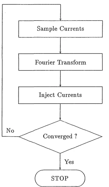
IRA (Iterative Harmonic Analysis) is a general technique for solving for the harmonic generation of a non-linear device. It is essentially a frequency domain technique, al-though, for practical devices with switching non-linearities, regular excursions are made into the time domain.

(23)

harmonic currents, which, in turn, may be used to re-evaluate the terminal voltage distortion. Thus, an iterative structure becomes apparent, as shown in figure 1.2.

Sample Currents

Fourier Transform

Inject Currents

No

Converged?

Yes STOP

Figure 1.2: Structure of IHA algorithm

The number of iterations required depends on a number of factors, but the most important of these are the nature of the non-linearity and the harmonic impedance of the supply network. It is intuitively apparent that if either the device is particularly sensitive to the presence of distortion, or the harmonic impedances are particularly high, then the solution will take longer to converge.

[image:23.568.188.374.147.466.2]

(24)

1.3 THE PRESENT WORK

This chapter has briefly described the causes and effects of harmonics in the power system. Three harmonic analysis techniques for RVDC convertor plant have been described and compared in, at least, a primitive sense. Of these three techniques (EMTDC, TCS, IRA), IRA appears-to be best suited to the harmonic analysis, since this is its primary purpose, and since it doesn't suffer from the drawback of the time domain methods.

The next chapter discusses the application of IRA specifically to the RVDC con-vertor, and sets down the quasi-steady state equations which describe the convertor operation.

Chapter 3 is devoted to an examination of the facts surrounding divergence of IRA, and its physical interpretation. Particular attention is given to developing a 'theory' which (in principle) unifies all cases of divergence.

Chapter 4 develops a new three phase integrated load and harmonic flow algorithm based on existing three phase analysis tools, and employing the IRA algorithm as a

fundamental part of it. A set of simple test cases are examined to assess the nature of

the integrated algorithm.

Chapter 5 applies the integrated algorithm to a pair of systems pertinent to the New Zealand situation, both of which serve to justify the development and use of the new technique. In particular, harmonic interactions between remote harmonic sources are examined in the New Zealand context, thus opening a new field of potential research.

(25)

CHAPTER 2

APPLICATION OF IHA TO THE CONVERTOR

2.1 INTRODUCTION

The application of IHA to the convertor is by no means new, but may be traced back (in admittedly cruder form) to the late 1960s. Reeve et

at.

(1971) were among the first to describe the method, and it was quickly recognised by others.

Research into the topic at Canterbury began with the work of Harker (1980) who first formulated the problem here, and was subsequently extended by Eggleston (1985), who investigated a number of applications.

However, before detailing the mathematical model of the convertor, the general steady state operation of the standard 6-pulse convertor will be reviewed.

2.2 CONVERTOR OPERATION

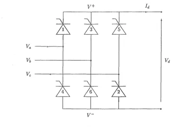
The Graetz bridge is the universal building block of most convertor schemes, and con-sists of 6 valves (or thyristors) connected as shown in figure 2.1

The numbering on the valves is the firing order, and is based on the order in which the valves become forward biased. The emphasised valves (1 & 2) are assumed to be conducting at the instant shown, and, as such, the d.c. current is supplied from phase 'a', and returns via phase 'c', while the d.c. voltage, Vd, is the instantaneous difference between Va and Ve.

The next valve to conduct (valve 3) may be fired at any instant during the interval it is forward biased, or, in other words, while Vb exceeds Va. When this happens, V+ begins to follow Vb, and since it is greater than Va, then current in phase 'a' reduces to zero. As depicted in figure 2.1, with no supply impedance, this process, known as commutation, would occur instantaneously, and therefore the current in phase 'a' would be a rectangular pulse, lasting from the firing of valve 1 to the firing of valve 3. The commutation process takes place 6 times per fundamental frequency cycle, and it

is analysis of this process in the presence of arbitrary distortion which is fundamental to the application of IHA to the convertor.

2.2.1 Commutation Process

(26)

v-Figure 2.1: The basic Graetz bridge.

it would be with adequate filtering), then the principal role in the commutation process is played by the reactance of the convertor transformer.

If the situation of figure 2.1 is taken and redrawn at the instant of firing of valve 3,

[image:26.573.103.455.81.341.2]

with transformer leakage inductances represented, then the configuration of figure 2.2 results.

Figure 2.2: Equivalent circuit of the commutation process.

Applying Kirchoff's Voltage Law around the loop gives

(2.1)

(27)

I dib 1 dia

Vba = bdi - aTi (2.2)

Applying Kirchoff's Current Law at the common cathode V+ :

(2.3) and if Id is assumed to be reasonably flat, as would be the case with sufficient

smoothing reactance in the d.c. circuit, then:

dia dib _ 0

dt

+

dt - (2.4)

or

(2.5) and therefore

(2.6)

Solution of this equation is given by

(2.7)

and

(2.8)

where lab is the sum of the leakage inductances of the 2 phases, and r

=

0 at the firing instant of valve 3.

The above equation is, of course, only valid during the commutation, since, when

ia is completely extinguished, valve 1 ceases to conduct, and can only be restarted by

the application of a firing pulse while forward biased. Note also that at r

=

0 the full load current is flowing in valve 1 (Le. in phase 'a') and therefore ib(O)

=

O.

For a purely sinusoidal supply Vba( r)

=

1fba sin (wr

+

a), where a is the firing delay

measured from the zero crossing of Vab, the solution becomes: ib( t)

=

ViZ'ba

rt

sin (wr

+

a) dr

ab

J

o 11b

-Za [-cos(wr+a)]~

w ab

Vba [cos(a) - cos(wt

+

a)] Xab

where Xab is the sum of the transformer reactances of the 2 phases.

The commutation concludes when ib(t)

=

Id, or, in other words, when Idxab

cos(wt

+

a)

=

cos(a) ,

-Vba

(2.9)

(28)

Note that for Xab

=

0, i.e. no commutating reactance, cos(wt

+

a)

=

cos( a), and

therefore the commutation is instantaneous. As eith~r Id or Xab increase, the

commuta-tion period lengthens, while for increasing commutating voltage (Vba) the commutation

period shortens.

The potential at the common cathode point (V+) during the commutation is given by:

(2.11) but since din.. -_{dt -} _11k _dt'

(2.12) which has the physical interpretation that v+ follows the average of the 2 phase voltages, provided that the commutatinginductances are equal. Since ib is the incoming phase,

*

>

°

during the commutation, and therefore v+ is reduced for

h

>

la, and

increased for

h

<

lao

In each complete cycle there are 6 commutations, and therefore 6 periods of steady conduction. These are given in figure 2.3, which depicts one complete cycle of rectifi-cation, with points labelled as they will be referred to in the mathematical description of the convertor. Briefly, they are:

ZCi - the point in time at which valve i becomes forward biased.

ai - the delay between ZCi and the firing instant of valve i. Bi - the instant in time at which valve i is fired.

i.e. Bi = ZCj

+

ai

J-li - the time taken for valve i to commutate on.

2.3 MATHEMATICAL MODEL OF THE CONVERTOR.

The mathematical model of the convertor is determined by certain practical require-ments. Provision must be made for accurate transformer models, and for the presence of distortion on both sides of the convertor. Since the purpose of the convertor model is to provide an updated estimate of its current waveform, a (quasi) steady state model is required, which takes as input the voltage distortion at the terminal busbar, and the current flowing on the d.c. side, and produces, as output, the a.c. current waveforms and the d.c. voltage waveform for the given input conditions.

2.3.1

Current Waveforms.

(29)

v

"

/ f '

'"

V-

i-"""

"

/

~

<

"

K

/

'"

1/

/

_~

"

/

"-

/ /

'\

V

'\

/

'\

/

[>

<

~

<

~

<

~

V

~

V

~

/'"

...

,../'"

...

/

F"'

~

Ix

~

i~(t)

iX

Ix

~

Figure 2.3: One cycle of rectification.

2.3.1.1 Commutating Current.

In order to calculate the commutating current in the presence of distortion, the distorted commutating voltage must be referred to the secondary of the convertor transformer. In so doing, the transformer is essentially 'split' into an ideal transformer (representing winding arrangements and off-nominal taps only) in series with its leakage impedance, with the referred commutating voltages in between. This may be more easily visualised with reference to figure 2.4.

Mathematically the process of referring the harmonic voltages across the trans-former, for the two of the most common winding arrangements, is accomplished as follows.

The primary voltages are given by :

Va(t)

2:

Va sin(hwt

+

¢~)

h

Vb(t)

2:

Vb

sin(hwt

+

¢~)

(30)

Ideal 0.05 pu Transformer I

a:1 a:1

Figure 2.4: Separation of the transformer into (ideal) winding configuration plus leakage

Vc(t)

=

I:Vcsin(hwt+4>~)

(2.13)

h

where Yah, vch, Vch,¢~,¢~,¢~ are the peak magnitudes and phases of the hth har-monic on phases 'a', 'b' and 'c' respectively.

L,h

indicates summation over all relevant harmonics, h.

For the case of a star-star transformer, the winding configuration is given in fig-ure 2.5.

Figure 2.5: Star-Star transformer winding configuration.

The time functions of the voltages referred to the secondary are therefore :

~

I:

Yah sine hwt

+

4>~)

-

~

I:

Vch sine hwt

+

4>~)

aa h ac h

~

I:

Vbh _sine_hwt

+

¢~)

_-

~

I:

_Yah_sine_hwt

+

¢~)

% h ~ h

~

I:

Vch sine hwt

+

¢~)

-

~

I:

Vbh sine hwt

+

¢~)

ac h ab h

(2.14)

(31)

Va

Vae

Yba

Vb Veb

Vc

Figure 2.6: Star-Delta transformer winding configuration.

-12:17: sin(hwt

+

cp~)

aa h

-1

2:

17bh _sin(hwt

+

cp~)

ab h

(2.15)

The commutating on of a valve, and the attendant commutating off of another, is modelled using a similar technique to that demonstrated earlier in the chapter, where the commutation current of phase 'b' was shown to be

(2.16)

In the presence of harmonics the purely sinusoidal Vba( T) is replaced by its harmonic

series

Lh

Vb~ sin(hwT

+

cpga),

where Vb~ and

cpga

are derived from equation 2.14 or 2.15

as appropriate.

Therefore, the commutating current in phase 'b' is given by :

1-

~t

2:

1fb~

sine hWT

+

CP~a)

dT

ab}~

h

+

rw

t

2:17b~

sin(hwT

+

cpga)

d(wr)

W ab }03 h

[

A h

]wt

~

-2::

1a COS(hWT

+

CP~a)

Xab h 1>3

~

[2::

1~

[COS(hB3

+

cpga) -

cos(hwt

+

cpga)]]

Xab h

(2.17)

which has a similar form to that given for the case where harmonics are ignored.

Similar equations hold for phases 'a' & 'c' with a cyclic change of suffices:

(2.18)

(32)

Alternatively, if some resistance is to be explicitly included in the commutating impedance, then the equation derived by Yacamini and de Oliveira (1986) may be used. This equation is given by :

where

50

in(t)

=

IJXhe-t/Tnm

+

Sh sin(hwt

+

(Ph))

+

Y(1 - e-t/ Tnm )

+

_{C nm}

h=l

Y

Bh Hh -1/Tnm Lnm h2_w2

+

_1/T;m

Bh H'K

+

h2_w2

hwLnm h2_w2

+

_1/T;m

Rm1d Rnm

n is the incoming phase number, m is that of the outgoing phase and

Rn+Rm Ln+Lm

Lnm/Rnm

Vhn cos(hBn

+

¢hn) - Vhm cos(hB,n

+

¢hm) Vhn sin(hBn

+

¢hn) - Vhm sin(hBn

+

¢hm)

hwAh/Bh

tan-1(h

~

)-tan-1(H hh)

w nm W

(2.20)

where Vhn & ¢hn are the magnitude and phase of the hth harmonic of the phase to neutral voltage of the incoming phase, and Vhm & ¢hm are similarly defined for the outgoing phase. Cnm is an integration constant such that in(O)

=

O.

Whichever equation is used, the instantaneous current in the phase that is commu-tating off is given by :

(2.21) where

ioff(t)

and

ion(t)

are the currents in the commutating off and commutating on phases respectively, and id(t) is the instantaneous d.c. current, given by :

id(t)

=

Id

+

'2:Jj

sin(hwt

+

¢j)

(2.22)

h

where Id is the d.c. component of the d.c. current, and Jj &

¢j

are the hth harmonic components of ripple in the d.c. current.

(33)

2.3.1.2 Steady Conduction

During periods of steady conduction (and at least one phase is conducting steadily at all times) the current flowing in that phase is that current flowing on the d.c. side of the convertor, as given in equation 2.22, with a positive sign if that phase is connected to the common cathode point, and a negative sign if connected to the common anode. During periods of non-conduction, the current in the non-conducting phase is set to zero.

2.3.1.3 Assembling the Current Waveforms

The current waveforms are sampled at regular intervals, beginning at wt

=

(h -

the firing instant of valve 1. The reason for this is that the conducting state of all valves and all phase currents are well defined at this instant. Inherent in this logic is the. assumption that no commutation will last more than 60°.

The process of sampling the currents is described by table 2.1, which gives the instantaneous values of each of the phase currents, with the limits between which the values are valid.

Limits Phase A current Phase B current Phase C current B1 B1

+

/11 ia(t) -id(t) id(t) - ia(t)

B1

+

/11 B2 id(t) -id(t) 0

B2 B2

+

/12 id(t) -id(t) - ic(t) ic(t)

B2

+

/12 B3 id(t) 0 -id(t)

B3 B3

+

/13 id(t) - ib(t) ib(t) -id(t)

B3

+

/13 B4 0 id(t) -id(t)

B4 B4

+

/14 ia(t) id(t) -id(t) - ia(t)

B4

+

/14 B5 -id(t) id(t) 0

B5 B5

+

/15 -id(t) id(t) - ic(t) ic(t)

B5

+

/15 B6 -id(t) 0 id(t)

B6 B6

+

/16 -id(t) - ib(t) ib(t) id(t) B6

+

/16 B1

+

211" 0 -id(t) id(t)

Table 2.1: A.C. current waveform sampling process.

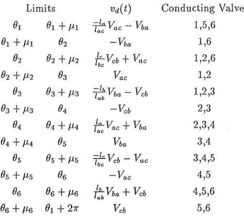
2.3.2 The D.C. Voltage

At the same time as the current waveforms are sampled, the d.c. voltage waveform may also be sampled, since it may be divided up into the same 12 periods of conduction and commutation.

(34)

commutating impedance, which is justified because the current flowing during steady conduction is essentially flat, and therefore the only voltage drop is across the resistive component of the impedance.

During commutations, there are 3 valves conducting, and calculation of the d.c. voltage is more complex. The approach used here is similar to that used in the single frequency case, described earlier.

Figure 2.7 depicts the situation with valve 1 commutating to valve 3.

Figure 2.7: Calculation of D.C. voltage during commutation.

From figure 2.7 it can be seen that:

(2.23)

where vx(t) = h~. Applying Kirchoff's Voltage law around the commutating loop,

(2.24)

so that

(2.25)

and therefore

(2.26)

where Vba(t) and Vcb(t) are represented by the harmonic time series described earlier.

The 12 sections of the d.c. voltage waveform, therefore, are given in the table 2.2.

2.4 SOLUTION TECHNIQUE.

The steady state harmonic generation of the convertor is solved using the IRA technique

(35)

Limits

Vd(t)

Conducting Valves

(h

+

J.L1 .=1.. I _aeV; ae -

Vi

ba 1,5,6

B1

+

J.L1 B2 -Vba 1,6

B2 B2

+

J.L2 fc-Veb _be

+

Vae 1,2,6

B2

+

J.L2 B3 Vae 1,2

B3 B3

+

J.L3 =lb.V; I ba - V; cb 1,2,3

ab

B3

+

J.L3 B4 -Vcb 2,3

B4 B4

+

J.L4 fa-Vae _ae

+

Vba 2,3,4

B4

+

J.L4 Bs Vba 3,4

Bs Bs

+

J.Ls =.1.0. _I V; _{eb -} V; _ae _3,4,5

be

Bs

+

J.Ls B6 -Vae 4,5

B6 B6

+

J.L6 fa-Vba _ab

+

Veb 4,5,6 [image:35.567.168.420.89.315.2]

B6

+

J.L6 Bl

+

21l" Vcb 5,6

Table 2.2: D.C. voltage sampling process.

parts: solution of the a.c. network, solution of the convertor operation and solution of the d.c. network.

Solution of the convertor operation (under arbitrary harmonic conditions) has been described in section 2.3, and needs little further elaboration, while the details of solving the a.c. and d.c. networks are given in sections 2.4.3 & 2.4.4.

Figure 2.8 is the flowchart of the IRA algorithm applied the the convertor, the steps of which are described more fully in the following sections.

2.4.1 Read Initial Conditions

The initial operating state of the convertor as determined by a loadflow is read in. It

consists of the terminal busbar fundamental voltage magnitudes and phases (lfa,

Vb,

V

e, CPa, CPb, CPc), the commutating reactances (Xa,Xb,X e), the set of firing angles (O'i),

the d.c. current level

(Id),

the transformer taps

(ai)

and the transformer connection information. Also required are the a.c. and d.c. system harmonic admittance matrices.

2.4.2 Calculate A.C. Harmonic Currents

The a.c. current waveforms are sampled using the 12 section current model equations described in section 2.3, table 2.1. The three phases are sampled simultaneously with the d.c. voltage waveform, which is calculated using the 12 section d.c. voltage model described in section 2.3, table 2.2. The time domain waveforms are then transformed into the frequency domain using the Fast Fourier Transform (FFT) algorithm, yielding a cos series referenced to B1 , the firing instant of the first valve. T'his series is referred

(36)

No

Read Initial Conditions

Calculate A.C. harmonic currents, inject into &

solve A.C. network

Calculate D.C. harmonic voltages, impress on &

solve D.C. network

Converged?

Yes

STOP

Figure 2.8: Flowchart of the IRA process applied to the convertor.

2.4.3 Solution of the A.C. Network

The harmonic currents are injected into the a.c. system harmonic admittance matrices, one frequency at a time.

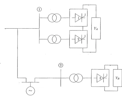
The size of the admittance matrices depends on 2 parameters: NT - the number of terminal busbars, and Nc - the number of convertors. A terminal busbar is one to which at least one convertor is connected (via a transformer), so that Nc

2:

NT always. For example, the sample system in figure 2.9 has 3 convertors, but they are connected to only 2 busbars - therefore NT

=

2 & Nc

=

3.

The admittance matrices for the a.c. system up to the terminal busbars are formed externally, and are of order 3NT X 3Nc -in figure 2.9 they are 6 X 6.

A 6 X 6 admittance matrix is formed for each convertor transformer (based on its leakage impedance and winding arrangement) and added to the system admittance matrices to give a composite matrix of size 3(NT

+

Nc) X 3(NT

+

Nc). The structure of this matrix for the example of figure 2.9 is as follows:

(37)

[image:37.570.89.491.87.406.2]

CD

Figure 2.9: Example of convertor interconnection.

0 _{Y n}

+

_{YP P1}

+

YPP2 Y 12 YPS1 YPS2 l1p1

0 _{Y 21} YZZ

+

YPP3 YPS3 VP2

11 YSP1 YSS 1 l1s1

12 YSP2 YSS 2 l1s2

h

YSP3 YSS3 l1s3

(2.27) where YPPi, YPSi, YSPi and YSSi are the primary-self, primary-secondary, secondary-primary and secondary-self three phase admittance matrices for convertor transformer i, and the terms Y ll , Y 12 /Y21 and Y zz are the self, mutual and self three phase nodal admittance matrices for terminal busbars 1 and 2 respectively. This is repeated for each frequency of interest.

The left hand side (LHS) excitation vector contains zero in the first two places, since the external harmonic injections take place at the convertor busbars only, while the right hand side (RHS) result vector contains the harmonic voltages at both the primary and secondary of the convertor transformer.

(38)

fo1'-ward & backward substitution to solve for the primary voltages VPi. The secondary harmonic voltages (VSi) are also found, but, being of little practical use, are discarded.

2.4.4 Solution of the D.C. Network

The d.c. voltage harmonics are impressed on the d.c. system impedance at each fre-quency, to give the harmonic currents flowing in the d.c. network. The d.c. system harmonic admittance matrix is formed externally, and therefore must contain the in-terconnection information for the d.c. network at harmonic frequencies. The matrix is

of order N c, and for the example of figure 2.9 has the following structure:

and the currents are found by simple matrix multiplication:

at each frequency h.

Yj

o

(2.28)

(2.29)

Since each set of V_d

1

is a sin series referenced to the system angle reference, the

harmonic currents found by solving equation 2.29 are also a sin series with the same angle reference. This must be accounted for when the d.c. current harmonics are used to calculate the instantaneous d.c. current values in the a.c. current and d.c. voltage sampling procedure.

2.5 CONVERGENCE

Convergence is said to have been obtained when the harmonics of successive iterations are sufficiently close that further iterations would yield no significant change. In other words, the harmonic voltages and currents form a self-sustaining set. Determining whether or not this condition has been reached can be accomplished in a number of ways.

Directly comparing the harmonic voltages of successive iterations is the most obvi-ous, with the advantage that every harmonic is individually inspected for convergence. However, it is difficult to assign a realistic tolerance to such a test: characteristic har-monics are generally present at a higher level than non-characteristic harhar-monics, which rules out the possibility of using some absolute tolerance level, such as, say 0.000001

pu, since different harmonics will converge to different levels. If a relative or percentage

(39)

Another way of determining convergence is to compare some suitable attribute of the two sets of harmonic voltages. One such attribute which has been used successfully in the past is the set of zero crossings, ZCi. These can be calculated from either the

commutating voltages or the phase voltages using a suitable numerical method, and taking, as initial conditions, the zero crossings from the previous iteration. When the shift in zero crossings between iterations reduces to below some tolerance, e.g. 0.0001 radians (~ 0.006°), then the harmonics are assumed to have converged. One advantage of this method which garnered much favour in earlier days was the efficient use of memory, since it is only necessary to retain 6 values per convertor (ZC1 - ZC6 ) from

the previous iteration, compared with up to 300 (3 phases, 50 harmonics per phase, real and imaginary values for each harmonic) values in the case of direct comparison. The major setback of this method is the susceptibility of the numerical method (typically a regula falsi method) used for recalculating the zero crossings to fail in the presence of distortion. This was originally assumed to be due to the presence of multiple zero crossings, indicating excessive distortion. However it can also be caused by 'flattening' of the commutating voltage during commutations, resulting in a near zero slope on the voltage waveform which confuses the numerical method.

The method adopted throughout most of this thesis is a combination of the direct comparison and attribute comparison techniques, since it requires the previous iteration harmonic voltages to be retained, but only uses three attributes (one per phase) to ascertain convergence or otherwise. The attribute for each phase i at iteration k is defined as :

ti

=

L

IlVih,k _ Vih,k-11lIlVih,kll

+}Vih'k-lll

h

(2.30) which corresponds to summing the magnitudes of the phasor differences between successive iterations, weighted by the average of the two phasor magnitudes, so that more weight is assigned to the larger harmonics, less to the smaller ones. Convergence is assumed when all the convergence attributes have reduced to less than 0.001 of their original values, where the original values are those calculated on the first iteration, and therefore measure the impact of the introduction of the harmonics. This method has the advantage that it is relatively insensitive to 'noise level' harmonics (since they are small in magnitude) and a tolerance level is assigned which adapts to the particular case. For example, using an absolute tolerance level on a system with low harmonic distortion would result in very few iterations before apparent convergence, with the result that full harmonic interaction may not have taken place. Conversely, in a system with high harmonic distortion, the convergence criterion might never be satisfied, even though the harmonic interaction had been adequately solved.

2.6 SIMPLE TEST SYSTEM

The following simple example (figure 2.10) is cited to demonstrate the validity of the IHA technique applied to the static convertor. The solution may be obtained by 2 methods: IHA and direct solution.

(40)

E

=

1.0LO°

Vf

L<ph 0.15 pu Id

=

1.0pu [image:40.573.96.508.376.597.2]

0.05 pu

Figure 2.10: A simple test system.

is used (with a and E) to calculate the current waveform in each phase. These are

transformed into the frequency domain using an FFT, and are then used to calculate the harmonic voltages at the terminal busbar. As the presence of distortion in the

current waveform does not affect E (it is a perfect voltage source) the solution need

proceed no further.

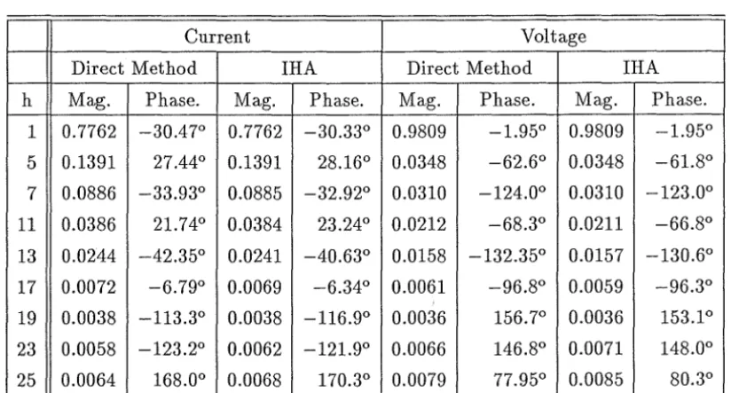
The fundamental conditions from the direct method (the terminal busbar funda-mental voltage and the effective delay angle measured with respect to it) are used to fuel the IRA technique. The characteristic harmonics are compared in table 2.3.

Current Voltage

Direct Method IRA Direct Method IRA

h Mag. Phase. Mag. Phase. Mag. Phase. Mag. Phase.

1 0.7762 -30.47° 0.7762 -30.33° 0.9809 -1.95° 0.9809 -1.95°

5 0.1391 27.44° 0.1391 28.16° 0.0348 -62.6° 0.0348 -61.8°

7 0.0886 -33.93° 0.0885 -32.92° 0.0310 -124.0° 0.0310 -123.0°

11 0.0386 21.74° 0.0384 23.24° 0.0212 -68.3° 0.0211 -66.8°

13 0.0244 -42.35° 0.0241 -40.63° 0.0158 -132.35° 0.0157 -130.6°

17 0.0072 -6.79° 0.0069 -6.34° 0.0061 -96.8° 0.0059 -96.3°

19 0.0038 -113.3° 0.0038 -116.9° 0.0036 156.7° 0.0036 153.1°

23 0.0058 -123.2° 0.0062 -121.9° 0.0066 146.8° 0.0071 148.0°

25 0.0064 168.0° 0.0068 170.3° 0.0079 77.95° 0.0085 80.3°

Table 2.3: Comparison of Direct and IRA solutions for a simple case.

The effective firing angle used in the IRA solution is simply the firing angle with

respect to the perfect source E, modified by the phase shift between E and the terminal

busbar, i.e.

(41)

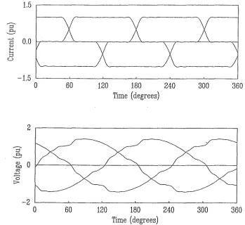
phase voltages and currents are given in figure 2.11.

1.5

1::

_Q.) 0.0

H

8

u

-1.5

2

-2

o

60

120

180

240

Time (degrees)

o

60

120

180

240

Time (degrees)

300

360

[image:41.567.102.451.111.431.2]

300

360

Figure 2.11: Reconstructed waveforms from the IHA results of the simple test system. The similarity between the results of IHA and the direct method prove that IHA is eminently suited to this type of analysis, and a convergent solution is very accurate indeed. This imparts a considerable degree of confidence in the iterative approach, which is necessary, since most practical situations preclude verification with the direct method. For example, the presence of only one simple shunt component between the source voltage E and the convertor would prevent the direct method from being used.

2.7 CONCLUSIONS

This chapter has been concerned with developing the mathematical theory of steady-state Graetz bridge operation such that it may be used within the iterative structure of the general IHA algorithm described in chapter 1.

(42)

Inclusion of the convertor transformer has been achieved by incorporating it into the admittance matrix of the supply network, and the general structure of the admittance matrices on both the a.c. and d.c. sides of the bridge have been derived to complete the description of the application of IRA to the convertor.

The criteria by which convergence may be measured have been discussed, and a method based on a combination of direct comparison and attribute comparison has

been selected on the basis that it could adapt itself to suit a particular situation.

Finally a simple test system has been solved by both IRA and a direct solution (to which it was readily adaptable) and the comparison of results was sufficiently good to inspire confidence in the converged IRA solution.

(43)

CHAPTER 3

INSTABILITY IN ITERATIVE HARMONIC ANALYSIS

3.1

INTRODUCTION

Since its introduction in simple form in the early seventies, IHA has been shown to be an accurate means of assessing the harmonics of non-linear devices, including static power convertors (Reeve et ai., 1971; Yacamini and de Oliveira, 1980) and transformers

in saturation (Dommel et ai., 1986). More recent work has favourably compared the

IHA .algorithm to an equivalent time domain simulation and to an analytically solvable system with excellent results, verifying not only the formulation of the IHA approach, but also of the time domain study (TCS) (Arrillaga et al., 1987). However, if the

algorithm should fail to converge, as it is known to do, then an explanation is required; especially so if the operating conditions are reasonable.

Most mathematical algorithms can be shown to be unstable in certain situations, and these situations determine the suitability of the algorithm to the application. Time domain simulations involving step-by-step integration of the system differential equa-tions can become unstable when the integration algorithm used is not compatible with the form of the solution. Use of finite precision arithmetic is also a problem, since any error in the calculation of the next solution point will (generally) be carried forward into the calculation of subsequent points. Similar considerations are likely to apply to IHA type algorithms, as is the observation that a genuinely unstable situation would be reflected to some degree in the performance of the algorithm.

The term 'harmonic instability' is defined by both Ainsworth (1981) and Arril-laga (1983) as being magnification of non-characteristic frequencies by a convertor sys-tem containing, initially, no unbalance or asymmetry, and there have been a number of examples of harmonic instabilities reported in the context of HVDC transmission in re-cent years. Holmborn and Martensson (1966) reported on a third harmonic instability which often developed in the Cross-Channel link under certain a.c. system conditions, rendering the link inoperable. This problem was alleviated by the inclusion of a third harmonic filter - a solution which was adopted at the design stage of the Sardinian HVDC terminal (Natale et ai., 1966). A similar problem, although this time related to

the second harmonic, was found to exist in the Kingsnorth scheme (Last et al., 1966).

Within New Zealand, excessive ninth harmonic was observed at the Benmore terminal of the New Zealand HVDC interconnection, and a ninth harmonic filter was necessary to solve this problem (Robinson, 1966). Kauferle et ai. (1970) characterised harmonic

instabilities by the excessive levels of harmonic distortion associated with them, often rendering the link inoperable.

(44)

only to refer to a case where the physical system is harmonically unstable, and cases in which IHA fails to converge will be termed 'algorithmically unstable'.

3.1.1 Review of IRA Research

Prior to 1970, the topic of convertor harmonics was approached by considering aspects of harmonic generation separately. Commutating impedance unbalance was analysed separately from terminal voltage unbalance, and the effects of controllers considered separately again. In fact Rissik (1939) described in the late thirties many of the har-monic phenomena still under investigation today.

Reeve and Baron's algorithm (Reeve et at., 1971) was virtually the earliest

applica-tion ofIHA to the convertor, and, although somewhat cruder than current formulaapplica-tions, apparently still suffered from problems of convergence. This was seen by the authors as indicating either an harmonic instability, or at least a potantial harmonic instability. Yacamini and de Oliveira described their formulation of the algorithm in 1980 (Ya-camini and de Oliveira, 1980), and were clear in their statement that if the IHA al-gorithm failed to converge, then the physical system would suffer from a harmonic instability. They also claimed that their algorithm did not suffer from " ... problems of numerical instability ... ", although in this, it is more likely that they were referring to the type of numerical problems experienced in time domain simulation.

Bruce Harker developed a simplified version of IHA at Canterbury (Harker, 1980), and investigated a third harmonic resonant condition which demonstrated the phase angle controller as being inferior to the symmetrical firing controller in terms of un-characteristic harmonic generation, and showed the phase angle controller to render the algorithm unstable if the third harmonic resonance was approached too closely. In his conclusions, he stated that there was significant uncertainty in the numerical solution for uncharacteristic harmonics, this being due to the inherent sensitivity to a wide range of parameters which were difficult to assess, or were of a time-varying, rather than steady-state nature.

Eggleston (1985) developed and extended the algorithm formulated by Harker, and in his investigations isolated the third harmonic as the root of many of the algorithmic instabilities. He also demonstrated that, at least in a particular case, the algorithmic instability exhibited behaviour characteristic of an harmonic instability in that it was independent of the system impedance unbalance, and could be removed by filtering or reducing the power of the convertor. Attempts at improving the numerical technique were also unsuccessful, which would also be characteristic of a true harmonic instabil-ity, since the instabilty would depend on the physical system parameters and not the simulation technique. However, he was unable (or un willing) to state that there ex-isted a complete isomorphism between algorithmic instability and harmonic instability. Partly this may have been due to the fact that IHA was compared favourably with a time domain simulation (TCS) and both were shown to be accurate. However, when the TCS algorithm was applied to an unstable IRA case, a steady state solution was reached, indicating that the system didn't suffer from an harmonic instability.

(45)

general terms, it aims to unify the explanations into a theory which explains, in prin-ciple at least, all cases of algorithmic instability. The particular topics which will be addressed are :

@l Uncharacteristic harmonic production.

@l Growth of uncharacteristic harmonics.

@l Representation of dynamics.

@l Uncharacteristic harmonics with balanced systems.

3.2

UNCHARACTERISTIC HARMONIC PRODUCTION

It is a well documented fact that convertors under unbalanced operating conditions

produce harmonics which are uncharacteristic of their 'ideal' operation (Phadke and Harlow, 1968; Reeve and Krishnayya, 1968). The basic building block of the convertor

installation is the 6-pulse bridge, which normally produces harmonics of order 6k

±

1. If half wave symmetry is assumed, then even harmonics are not produced, and

the remaining uncharacteristic harmonics are those odd multiples of 3 - the triplen harmonics.

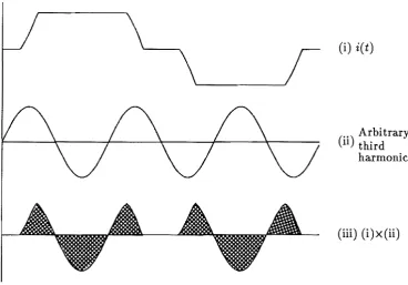
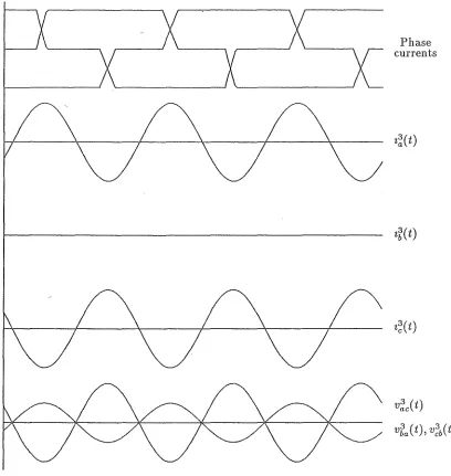
The reason that the triplen harmonics are not produced under ideal conditions is explained by considering an idealised phase current waveform over one cycle, compared with an arbitrary third harmonic waveform over the same period, as shown in figure 3.1. The bottom waveform is obtained by multiplying the two upper waveforms together. The proportion of third harmonic in the phase current waveform is proportional to the total shaded areas of the composite waveform, since

1

121r

b3

= -

f(

8) sin(38

+

¢ )dB

7r 0

is the third harmonic component of the (arbitrary) function

f(8).

The problem is simplified by appealing to half-wave symmetry, so that the

contri-bution of the second half cycle is equal to that of the first. Assuming the pt and 3rd

commutating-on current waveshapes to be governed by functions ic1 (8) & ic3( 8)

respec-tively, and that the steady conduction current is Id then the third harmonic component

IS :

~

r

i(B) sin(38

+

¢)dB

7r

Jo

2

[lo~+~

lo~

- ic1(8) sin(38

+

¢)d8

+

Id sin(3B

+

¢)dB+

7r ~ ~+~

r~+~

1

J0

3

(Id - ic3(8)) sin(3B

+