Global Convergence of an Extended Descent Algorithm without Line Search for Unconstrained Optimization

http://www.scirp.org/journal/jamp ISSN Online: 2327-4379

ISSN Print: 2327-4352

DOI: 10.4236/jamp.2018.61013 Jan. 16, 2018 130 Journal of Applied Mathematics and Physics

Global Convergence of an Extended Descent

Algorithm without Line Search for

Unconstrained Optimization

Cuiling Chen

*

, Liling Luo, Caihong Han, Yu Chen

College of Mathematics and Statistics, Guangxi Normal University, Guilin, China

Abstract

In this paper, we extend a descent algorithm without line search for solving unconstrained optimization problems. Under mild conditions, its global con-vergence is established. Further, we generalize the search direction to more general form, and also obtain the global convergence of corresponding algo-rithm. The numerical results illustrate that the new algorithm is effective.

Keywords

Unconstrained Optimization, Descent Method, Line Search, Global Convergence

1. Introduction

Consider an unconstrained optimization problem (UP)

( )

min ,

n

x f x

∈ℜ (1)

where f :ℜ → ℜn is a continuously differentiable function. In general, the

iterative algorithms for solving (UP) usually take the form:

1 ,

k k k k

x+ =x +α d (2)

where xk,αk and dk are current iterative point, a positive step length and a search direction, respectively. For simplicity, we denote ∇f x

( )

k by gk and

( )

k

f x by fk.

The main task in the iterative formula (2) is to choose search direction dk and determine step length αk along the direction. There are many classic methods to choose search direction dk, such as the steepest descent methods, Newton-type methods, Variable metric methods (see [1]), and conjugate gradient methods

How to cite this paper: Chen, C.L., Luo, L.L., Han, C.H. and Chen, Y. (2018) Global Convergence of an Extended Descent Algo-rithm without Line Search for Uncon-strained Optimization. Journal of Applied Mathematics and Physics, 6, 130-137.

https://doi.org/10.4236/jamp.2018.61013

Received: December 16, 2017 Accepted: January 13, 2018 Published: January 16, 2018

Copyright © 2018 by authors and Scientific Research Publishing Inc. This work is licensed under the Creative Commons Attribution International License (CC BY 4.0).

http://creativecommons.org/licenses/by/4.0/

DOI: 10.4236/jamp.2018.61013 131 Journal of Applied Mathematics and Physics

{

1

if 1,

if 2,

k k

k k k

g k

d

g β d − k

− =

= − + ≥ (3)

where βk is a parameter (see [2] [3] [4]). For step length αk, it is usually determined by line search procedure, such as exact line search, Wolfe line search, Armijo line search, and so on. However, these line search procedures may involve extensive computation of objective functions and its gradients, which often becomes a significant burden for large-scale problems. Evidently, it is a good idea that line search procedure is avoided in algorithm design in order to reduce the evaluations of objective functions and gradients.

Based on the above consideration, some authors have started to study the algorithms without line search. Recently, some conjugate gradient algorithms without line search were investigated. In [5], Sun and Zhang studied some well-known conjugate gradient methods without line search, for instance, Fletcher-Reeves method, Hestenes-Stiefel method, Dai-Yuan method, Polak- Ribière method and Conjugate Descent method. In [6], Chen and Sun researched a two-parameter family of conjugate gradient methods without line search. In [7] [8], Wang and Zhu put forward to conjugate gradient path methods without line search. Shi, Shen and Zhou proposed descent methods without line search in [9] and [10], respectively. Further, Zhou presented the steepest descent algorithm without line search in [11].

Inspired by the above literatures, in this paper we will extend the descent algorithm without line search of [10] to more general case, and discuss its global convergence. The rest of this paper is organized as follows. In Section 2, we describe the extended descent algorithm without line search. In Section 3, we analyze its global convergence. Further, we generalize the search direction to more general form, and obtain global convergence of corresponding algorithm. Finally, numerical results are reported in Section 4.

2. Extended Descent Algorithm

To proceed, we first assume that [2]

(H1) The function f has lower bound on £

{

|

( )

( )

1

}

n

x f x f x

= ∈ℜ ≤ _{, where}

1

x is available.

(H2) The gradient g is Lipschitz continuous in an open convex set  that contains £, i.e., there exists L>0 such that

( )

( )

, , .

g x −g y ≤L x−y ∀x y∈ (4) Now we give the extended algorithm.

Algorithm 2.1. Given a starting point x1, a positive constant , three parameters µ µ1, 2 and ρ such that 1 2

1

0 1

2

µ µ

< < < < _, 1 1

2≤ <ρ . Let k: 1= .

Step 1. If gk <, then stop; otherwise go to Step 2. Step 2. Compute

(

)

2

2 T

1

, 1,

, 2.

1 k k

k k k

k g

s _k

g g d

ρ

ρ

ρ ρ ₋

= 



=  _≥

 _{+ −}



DOI: 10.4236/jamp.2018.61013 132 Journal of Applied Mathematics and Physics Step 3. Set search direction

(

)

1 1

1

1 1

, 1,

1 1 , 2.

1 1

k k

k k k k k

k k

k k

s g k

d s s

g d k

α α

ρ ρ

α α

− −

−

− −

− =



 _{ }

=_−  

− + − ≥

   

 _{ + + }

 

 



(6)

Step 4. Compute step length by the following rule. When k=1, α_k is determined by Wolfe line search, i.e., it satisfies that

(

)

T

1 ,

k k k k k k k

f x +α d − f ≤µ α g d (7)

(

)

T T

2 .

k k k k k k

g x +α d d ≥µ g d (8)

When k≥2,

T 2, k k k

k k g d

L d

α = − (9)

where Lk satisfies that ρ ≤L Lk ≤m Lk and

{

m kk, =1, 2,

}

is a positive sequence which has a sufficient large upper bound.

Step 5. Set next iterative point

1 .

k k k k

x+ =x +α d (10)

Step 6. Set k:= +k 1, and go to Step 1.

Remark 2.1. Note that the formula of sk and dk in Algorithm 2.1 are the generalized forms of those in [10].

3. Global Convergence

Lemma 3.1. If Algorithm 2.1 generates an infinite sequence

{

x kk, =1, 2,

}

,

then all search directions dk are descent, and ∀ ≥k 2, it holds that 2

T

1

. 1

k k k

k g

g d ρ

α −

− ≥

+ (11)

Proof. If k=1, it is obvious that −g d1T 1=ρ g12>0. If k≥2, by (5) and (6), we have

(

)

(

)

(

)

2

T 1 1 T

1

1 1

2 1 2 T

1 1

2 1 2 T

1 1

2

1

1 1

1 1

1 1

1 1

. 1

k k k k

k k k k k

k k

k k

k k k k

k

k k

k k k k

k

k

k

s s

g d g g d

s

g g g d

s

g g g d

g

α α

ρ ρ

α α

α

ρ ρ ρ

α α

ρ ρ ρ

α ρ

α

− −

−

− −

−

− −

−

− −

−

 

− = _ − _ + −

+ +

 

 

= − _ − − _

+

 

≥ − _ + − _

+

= +

(12)

This completes the proof. 

Lemma 3.2 (Mean value theorem, see [1]). Suppose that the objective function f x

( )

is continuously differentiable on an open convex set , then

(

)

1

(

)

T

0 d ,

k k k k k k

DOI: 10.4236/jamp.2018.61013 133 Journal of Applied Mathematics and Physics where x xk, k+αdk∈,

n k

d ∈ℜ . If f x

( )

is twice continuously differentiable on , then

(

)

1 ₂

(

)

0 d ,

k k k k k k

g x +

α

d −g =

α

∫

∇ f x +t d

α

d t (14)

and

(

)

_{T 2} 1

(

)

_{T 2}

(

)

0 1 d .

k k k k k k k k k

f x +

α

d − f =

α

g d +

α

∫

−t d ∇ f x +t d

α

d t (15)

Lemma 3.3. ∀ ≥k 2,

2 2 2

1

3 .

k i

i k

d

ρ

g

≤ ≤

≤ ⋅

∑

₍₁₆₎

Proof. Where k≥2, it holds that

(

1−

ρ

)

s g dk kT k−1 =

ρ

(

1−sk

)

gk 2 by (5). Then ∀ ≥k 2, we have

(

)

(

)

(

)

(

)

(

)

2

2 _{1 1}

1

1 1

2 2

2 1 1

1 1 2 2 2 T 1 1 1 1 1 1 2 2 2 T 1 1 2 2 2 2 1 1 1 1 1

1 2 1

1 1

1 1

1 1

2 1

2 1

k k k k

k k k

k k

k k k k

k

k k

k k k k

k k k

k k

k k k k k

k k k k

s s

d g d

s s

g

s s

g d d

g s g d d

g s g d

α α ρ ρ α α α α ρ ρ α α α α ρ ρ α α

ρ ρ ρ

ρ ρ − − − − − − − − − − − − − − − − − −   =  −  + − + +       = _ − _ + _ − _ + +       ⋅ − ⋅ + − _{ } + _ + _ ≤ + − +

= + − + 2 2 2 2

1

3ρ gk dk− .

≤ +

Using induction principle and noting that 2 2 2

1 1

d =ρ g , it yields that

2 2 2 2 2 2 2 2 2

1 2 1

3 3 3 .

k k k k

d ≤ ρ g + ρ g₋ + ρ g₋ + + ρ g

Therefore (16) holds. The proof is completed. 

Theorem 3.1. If (H1), (H2) hold, and Algorithm 2.1 generates an infinite sequence

{

x kk, =1, 2,

}

, then

(

)

4 2 2 2 1 1 ; 1 k k k i i k g g α +∞ = ₋ ≤ ≤ < +∞ +

∑

∑

(17)

and 2 2 1 . 1 k k k k g α α +∞ = − < +∞ +

∑

(18)

Proof. When k≥2 , from (13), (4), Lemma 3.1, Lemma 3.3 and

k k

L L m L

ρ ≤ ≤ _{, it yields that}

(

)

(

)

(

)

1 T 1 ₀ 1 T T 0 1 T 0

1 2 2

T 2 T 2

0 d d d 1 d 2

k k k k k k k

k k k k k k k k k

k k k k k k k k k

k k k k k k k k k k

f f g x t d d t

g d g x t d g d t

g d g x t d g d t

g d L t d t g d L d

α α

α α α

α α α

α α α α

DOI: 10.4236/jamp.2018.61013 134 Journal of Applied Mathematics and Physics

(

)

(

)

(

)

(

)

(

)

(

)

(

)

2 2 T T

2 2 ₂ 2

4 2 2 2 2 2 1 1 4 2 2 2 1 1 2 1 1 1 2 2 2 1

2 1 3

2 1

,

6 1

k k k k

k k k k k

k

k k i

i k

k

k k i

i k

g d g d

L L d Lm d

g Lm g g Lm g ρ ρ ρ α ρ ρ α − ≤ ≤ − ≤ ≤ −   =_ − _ ≥   − ⋅ ≥ + ⋅ ⋅ − = +

∑

∑

(19)

which implies that

{

f kk, =1, 2,

}

is a decreasing sequence. And it is clear that

the sequence

{

x kk, =1, 2,

}

generated by Algorithm 2.1 is contained in 

by (H1), and there exists a constant f* such that limk→∞ fk = f*. Therefore

(

)

(

)

(

)

*

1 1 2 1 2

2 2

lim lim .

N

k k k k N

N N

k k

f f f f f f f f

+∞ + _→+∞ + _→+∞ + = = − = − = − = −

∑

∑

Thus

(

1

)

2 , k k k f f +∞ + =

− < +∞

∑

which combining with (19) yields

(

)

4 2 2 2 2 1 1 . 1 k k

k k i

i k g

m α g

+∞ = ₋ ≤ ≤ < +∞ +

∑

∑

(20)

Since

{

m kk, =1, 2,

}

has an upper bound, (17) holds.

On the other hand, by (9) and Lemma 3.1, we have

(

)

(

)

(

)

(

)

(

)

(

)

2 T 2 1 T T T T 2 1 1 2 2 2 2

2 1 2 1

.

2 2 1

k k k k k k k

k k k k

k k k k k k

k k

k k k k k

k

f f g d L d

L L g d

L g d

g d

L L

g d g

α α

α α

α

ρ α _{ρ α}

ρ α + − − ≥ − − − = − + = − − − ≥ − ≥ + (21)

By the same analysis as the above proof, (18) holds. The proof is completed. 

Lemma 3.4 (see [12]). If the conditions in Theorem 3.1 hold and

{ }

1

supk≥ αk < +∞, then both the sequence

{

g kk, =1, 2,

}

and

{

d kk, =1, 2,

}

have a bound.

Theorem 3.2. If the conditions in Theorem 3.1 hold, then

lim infk→+∞ gk =0. (22)

Proof. Suppose lim infk→+∞ gk ≠0, then there exists a positive γ such that

, 1.

k

g ≥ ∀ ≥γ k (23)

In the following, we carry out our proofs in two cases.

Case 1. We complete the proof by utilizing reduction to absurdity. Suppose

DOI: 10.4236/jamp.2018.61013 135 Journal of Applied Mathematics and Physics 4

2 2

1 k

k _i

i k g

g

+∞

= ≤ ≤

< +∞

∑

∑

(24)

From Lemma 3.4, we know that there exists M >0 such that

, 1

k

g ≤M ∀ ≥k . Combining (23), we have

4 ₄

2 2

1

.

k

i i k

g

k M g

γ

≤ ≤ ≥

⋅

∑

It is known that

4 4

2 2

2 2

1 ,

k k M M k k

γ γ

+∞ +∞

= =

= = +∞

⋅

∑

∑

So

4 2 2

1

,

k

k

i i k

g

g

+∞

= ≤ ≤

= +∞

∑

∑

(25)

which contradicts with (24). Therefore (22) holds.

Case 2. When supk≥1

{ }

αk = +∞, the proof is the same as that in [10] and here is omitted.

It follows from the proofs of Case 1 and Case 2 that (22) holds. This completes the proof. 

Remark 3.1. Search direction of Algorithm 2.1 can be extended to more general form as follows:

(

)

(

1

)

(

) (

1

)

1

, 1,

1 1 , 2,

k k k

k k k k k k

s g k

d

s g s d k

ρ ϕ α ₋ ρ φϕ α _{− −}

− =



= − −_ ± − ≥ (26)

where the function ϕ α

( )

_{satisfies the following conditions(see [10]):}

a) It is continuous and strictly monotone increasing when α ∈

[

0,+∞

)

;

b) limα→0+ϕ α

( )

=ϕ

( )

0 =0 and limα→+∞ϕ α

( )

=1;

c) α

(

1−ϕ α

( )

)

is continuous, strictly monotone increasing when

[

0,

)

α ∈ +∞ _{, and}

( )

(

)

lim 1 1.

α→+∞

α

−

ϕ α

=

Evidently, there are many functions satisfying the conditions (a)-(c). For example,

1

α α

+ ,

2 2

1

α

α α

+ + ,

3

2 3

1

α

α

α

+ + , etc (see [10]). We denote Algorithm

2.1 in which dk is determined by (26) as Algorithm 3.1. By using proof technique of above Theorem 3.2, it is easy to get its convergence theorem.

4. Numerical Results

In this section, we report some preliminary numerical experiments. The test problems and their initial values are drawn from [13].

In numerical experiment, we take the parameter Lk =100,and stop the

iteration if the inequality 5

10

k

[image:7.595.208.541.88.350.2]

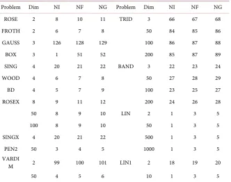
DOI: 10.4236/jamp.2018.61013 136 Journal of Applied Mathematics and Physics Table 1. Numerical results.

Problem Dim NI NF NG Problem Dim NI NF NG

ROSE 2 8 10 11 TRID 3 66 67 68

FROTH 2 6 7 8 50 84 85 86

GAUSS 3 126 128 129 100 86 87 88

BOX 3 1 51 52 200 85 87 89

SING 4 20 21 22 BAND 3 22 23 24

WOOD 4 6 7 8 50 27 28 29

BD 4 5 7 9 100 23 25 27

ROSEX 8 9 11 12 200 24 26 28

50 8 9 10 LIN 2 1 3 5

100 8 9 10 50 1 3 5

SINGX 4 20 21 22 500 1 3 5

PEN2 50 3 4 5 1000 1 3 5

VARDI

M 2 99 100 101 LIN1 2 18 19 20

50 4 5 6 10 1 3 5

are reported in Table 1, in which NI, NF and NG denote the total number of iterations, the total number of function evaluations and the total number of gradient evaluations, respectively. From Table 1, we can see the extended algorithm has good numerical results.

5. Conclusion

In this paper, we extended the descent algorithm without line search of [10] to more general case, and got its global convergence. Compared with [10], the extendedalgorithm has more effective numerical perfermance, so it is effective. In the future, we will further research the descent algorithms without line search, and try to get some new descent algorithms without line search, which not only convergence globally, but also have good numerical results.

Acknowledgements

We gratefully acknowledge the scholarship fund of education department of Guangxi Zhuang autonomous region, Guangxi basic ability improvement project fund for the middle-aged and young teachers of colleges and universities (2017KY0068, KY2016YB069), Guangxi higher education undergraduate course teaching reform project fund (2017JGB147), NNSF of China (11761014), Gua-ngxi natural science foundation (2017GXNSFAA198243).

References

DOI: 10.4236/jamp.2018.61013 137 Journal of Applied Mathematics and Physics

[2] Dai, Y.H. and Yuan, Y. X. (2000) Nonlinear Conjugate Gradient Methods.Shanghai Science and Technology Press of China, Shanghai. (In Chinese)

[3] Gilbert, J.C. and Nocedal, J. (1992) Global Convergence Properties of Conjugate Gradient Methods for Optimization. SIAM Journal on Optimization, 2, 21-42.

https://doi.org/10.1137/0802003

[4] Grippo, L. and Lucidi, S. (1997) A Globally Convergent Version of the Polak-Ribière Conjugate Gradient Method. Mathematical Programming, 78, 375-391.

https://doi.org/10.1007/BF02614362

[5] Sun, J. and Zhang, J.P. (2001) Global Convergence of Conjugate Gradient Methods without Line Search. Annals of Operations Research, 103, 161-173.

https://doi.org/10.1023/A:1012903105391

[6] Chen, X.D. and Sun, J. (2002) Global Convergence of a Two-Parameter Family of Conjugate Gradient Methods without Line Search. Journal of Computational and Applied Mathematics, 146, 37-45. https://doi.org/10.1016/S0377-0427(02)00416-8

[7] Wang, J.Y. and Zhu, D.T. (2016) Conjugate Gradient Path Method without Line Search Technique for Derivative-Free Unconstrained Optimization. Numerical Al-gorithms, 73, 957-983. https://doi.org/10.1007/s11075-016-0124-9

[8] Wang, J.Y. and Zhu, D.T. (2017) Derivative-Free Restrictively Preconditioned Conjugate Gradient Path Method without Line Search Technique for Solving Linear Equality Constrained Optimization. Computers and Mathematics with Applica-tions, 73, 277-293. https://doi.org/10.1016/j.camwa.2016.11.025

[9] Shi, Z. J. and Shen, J. (2005) Convergence of Descent Method without Line Search.

Applied Mathematics and Computation, 167, 94-107.

https://doi.org/10.1016/j.amc.2004.06.097

[10] Zhou, G.M. (2009) A Descent Algorithm without Line Search for Unconstrained Optimization. Applied Mathematics and Computation, 215, 2528-2533.

https://doi.org/10.1016/j.amc.2009.08.058

[11] Zhou, G.M. and Feng, C.S. (2013) The Steepest Descent Algorithm without Line Search for p-Laplacian. Applied Mathematics and Computation, 224, 36-45.

https://doi.org/10.1016/j.amc.2013.07.096

[12] Shi, Z.J. and Shen, J. (2005) A New Descent Algorithm with Curve Search Rule. Ap-plied Mathematics and Computation, 161, 753-768.

https://doi.org/10.1016/j.amc.2003.12.058

[13] Morè, J.J., Garbbow, B.S. and Hillstrom, K.E. (1981) Testing Unconstrained Opti-mization Software. ACM Transactions on Mathematical Software, 7, 17-41.