Capacity Limits and Performance Analysis of
Cognitive Radio With Imperfect Channel Knowledge
Himal A. Suraweera,
Member, IEEE
, Peter J. Smith,
Senior Member, IEEE
, and Mansoor Shafi,
Fellow, IEEE
Abstract—Cognitive radio (CR) design aims to increase spec-trum utilization by allowing the secondary users (SUs) to coexist with the primary users (PUs), as long as the interference caused by the SUs to each PU is properly regulated. At the SU, channel-state information (CSI) between its transmitter and the PU receiver is used to calculate the maximum allowable SU transmit power to limit the interference. We assume that this CSI is imperfect, which is an important scenario for CR systems. In addition to a peak received interference power constraint, an upper limit to the SU transmit power constraint is also considered. We derive a closed-form expression for the mean SU capacity under this scenario. Due to imperfect CSI, the SU cannot always satisfy the peak received interference power constraint at the PU and has to back off its transmit power. The resulting capacity loss for the SU is quantified using the cumulative-distribution function of the interference at the PU. Additionally, we investigate the impact of CSI quantization. To investigate the SU error perfor-mance, a closed-form average bit-error-rate (BER) expression was also derived. Our results are confirmed through comparison with simulations.
Index Terms—Average bit error rate (BER), channel capacity, cognitive radio (CR), partial channel-state information (CSI), quantized feedback.
I. INTRODUCTION
T
HE RADIO spectrum is one of the most valuable re-sources for wireless communications. Conservative spec-trum policies employed by regulatory authorities have created the perception of a spectrum shortage that has resulted in underutilization of the overall available spectrum for commu-nications. However, measurements performed by agencies such as the Federal Communications Commission has revealed that, at any given time, large portions of spectrum are sparsely occu-pied. Given this fact, new insights into the use of spectrum have challenged the traditional approaches to spectrum-management motivating research in cognitive radio (CR) technology for opportunistic use of the spectrum [1]–[5].Manuscript received May 21, 2009; revised October 19, 2009. First pub-lished February 22, 2010; current version pubpub-lished May 14, 2010. This work was supported by the Australian Research Council under Discovery Grant DP0774689. This paper was presented in part at the IEEE Global Communications Conference, Honolulu, HI, November/December 2009. The review of this paper was coordinated by Prof. H. Zhang.
H. A. Suraweera is with the Department of Electrical and Computer Engineering, National University of Singapore, Singapore 119260 (e-mail: [email protected]).
P. J. Smith is with the Department of Electrical and Computer Engi-neering, University of Canterbury, Christchurch 8140, New Zealand (e-mail: [email protected]).
M. Shafi is with Telecom New Zealand, Wellington 6011, New Zealand (e-mail: [email protected]).
Digital Object Identifier 10.1109/TVT.2010.2043454
The CR concept, which was first introduced by Mitola [1], refers to a smart radio that can sense the external electro-magnetic environment and adapt its transmission parameters according to the current state of the environment. According to the quantity, reliability, and type of information available to a CR system, it can adopt three different spectrum-sharing paradigms [6]. CRs can be designed to access parts of the primary user (PU) spectrum for their information transmission, provided that they cause minimal interference to the PUs in that band [2], [3]. This can be achieved in several ways. For example, according to one of the paradigms widely referred to as theinterweaveapproach in the literature, CRs can sense the spectrum and access it when an unused primary slot is detected. In another model, known as the underlayapproach, CRs can simultaneously coexist with the PUs, provided that they operate under a certain interference level as imposed by a regulatory agency. Limits on this received interference level at the primary receiver can be imposed with a long-term average or short-term peak constraint, e.g., [7].
Capacity analysis is very useful in understanding the per-formance limits and, thus, the potential applications of CR systems. Several interesting results on the capacity, outage probability, and throughput of CR systems have recently emerged. See, for example, [7]–[14], [16], and the refer-ences therein. In [8], the capacity of nonfading additive white Gaussian noise (AWGN) channels under an average received-power constraint at a primary receiver is derived. In [9], it was shown that, with the same limit on the received-power level, the channel capacity for several different fading models (e.g., Rayleigh, Nakagami-m, and lognormal fading) exceeds that of the nonfading AWGN channel. In [10], the ergodic, the outage, and the minimum-rate capacity gains offered by a spectrum-sharing approach under average and peak interference con-straints in Rayleigh fading environments have been studied. It has been shown in [10] that imposing a constraint on the peak received power on top of the average received-power constraint does not yield a significant impact on the ergodic capacity as long as the average received power is constrained. In [11], opti-mal power-allocation strategies to achieve the mean capacity and the outage capacity of the secondary user (SU)1 fading channel under different types of power constraints and channel-fading models have been investigated. The authors show that the SU capacity achieved is higher under the average constraint compared with the peak interference power constraint and that
1In the following, “cognitive radio” and SU will both be used to identify the
node that seeks access to the PU’s licensed spectrum.
fading in the channel between the SU transmitter and the PU receiver is beneficial for enhancing the SU ergodic and outage capacities. In [7], the author has compared the PU capacity loss under average and peak interference constraints. For the scenario considered in [7], the average interference constraint provides better PU performance. Considering that, in some situations, the PU spectral activity in the vicinity of the CR transmitter may differ from that in the vicinity of the cognitive receiver, in [12], the capacity of opportunistic spectrum acquisi-tion has been investigated. The links of a primary/secondary ra-dio environment could also experience different types of fading such as Rayleigh and line-of-sight (LoS) Rician fading. Under such LoS scenarios, in [13], we have investigated the ergodic capacity of spectrum sharing under average and instantaneous interference constraints. It has been shown that the SU mean capacity is sensitive to the type of fading on the SU–SU and SU–PU links, and depending on the fading type on either link, the capacity can be either larger or smaller compared with the case of symmetric non-LoS Rayleigh fading. In [14], assuming a pathloss shadow-fading model with multiple PUs and SUs, the system-level capacities of CR networks under an average interference power constraint have been investigated. Their results have shown that the uplink ergodic channel ca-pacity of a CR-based central access network can be relatively large when the number of PUs is small. Moreover, the au-thors have demonstrated the benefits of employing multiple-input–multiple-output (MIMO) technology for SU networks targeting urban area deployments where a large number of coexisting PUs are expected. In [15], the allowable transmit powers for single- and multiantenna SU systems are evaluated under different types of fading (Rayleigh and Rician) for the PU–PU link and assuming that a target outage performance is applied in the PU system. Specifically, it has been found in [15] that, for PU-PU paths with significant LoS, the total power allowed for a multiantenna SU system is higher than the power allowed for a single-antenna SU system. Hence, the multiantenna SU system achieves power and diversity gains.
References [7]–[14] have all assumed that the SU has full channel-state information (CSI) knowledge of the link between its transmitter and the PU receiver. However, in practice, obtain-ing full CSI is difficult, and often, only partial CSI information can be acquired. This important situation has been studied in [16] under certain conditions. While [16] looks at the impact of partial CSI on the capacity, it only does so under an average interference constraint. The use of such a constraint is relevant when a long-term interference-induced degradation is to be considered. This may involve modeling both fast-fading and shadow-fading components of the radio channel. When only fast fading (Rayleigh) is considered, an interference constraint based on peak interference is more relevant. Furthermore, our approach to the CSI imperfections is different from that in [16], as our model caters for a range of solutions from near-perfect to seriously flawed channel estimates.
Even if a genie provides perfect CSI at the receiver, it must be quantized into a limited number of levels before being fed back to the SU transmitter. This process effectively converts the perfect CSI into an imperfect CSI scenario. Therefore, analyzing the impact of CSI imperfections on the SU capacity
is the key motivation of this paper. We assume partial CSI knowledge of the SU–PU link possibly due to a combination of channel estimation error, mobility, feedback delay, and limited feedback. As in [11], we assume that the SU has a maximum transmit power threshold since all real power amplifiers have an upper limit on their transmit power.
In this paper, we make several contributions.
1) We develop a closed-form expression for the SU mean capacity when it is required to work under a peak interfer-ence constraint imposed by the primary. We determine the impact of imperfect CSI of the SU–PU link by examining the effect of this on the interference constraint and the SU mean capacity.
2) Compared with perfect channel knowledge, under imper-fect CSI, the SU transmissions may result in a higher than acceptable interference to the PU. Consequently, the PU may demand lowering of the SU transmit power and, in turn, cause the SU to absorb a capacity loss. We relate this loss to the extent of the CSI imperfections. To quantify this SU capacity loss, the cumulative distribution function (cdf) of the received interference at the PU is derived. 3) We enhance the aforementioned result by including the
impact of quantization levels on the CSI and determine the number of levels before a regime of diminishing gains sets in.
4) Given the interference constraints, we develop a closed-form expression for the uncoded SU average bit error rate (BER) that can be extended to different modulation schemes. This allows us to compare the BER behavior versus peak interference with the corresponding trend for SU mean capacity.
This paper is organized as follows: Section II introduces the system model. In Section III, we investigate the mean SU capacity, the statistics of the PU interference, and the quantization effects of the CSI. The average BER of the SU system is analyzed in Section IV. In Section V, numerical results supported by simulations are presented and discussed. Finally, we conclude in Section VI.
II. SYSTEMMODEL
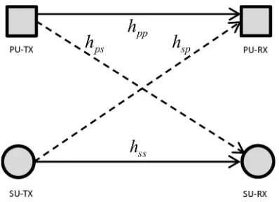
In this section, the system and channel models considered in the paper are briefly outlined. The system model is shown in Fig. 1. We assume that the PU and SU communication links share the same narrow-band frequency with bandwidth
B for transmission. Moreover, point-to-point flat Rayleigh fading channels are assumed. Let gsp=|hsp|2,gss =|hss|2, andgps=|hps|2denote the instantaneous channel gains from the secondary transmitter to the primary receiver, from the secondary transmitter to the secondary receiver, and from the primary transmitter to the secondary receiver, respectively. Fur-thermore, we denote the exponentially distributed probability density functions (pdfs) of the random variables (RVs) gsp,
gss, and gps by fgsp(x), fgss(x), and fgps(x), respectively.
These pdfs are governed by the parameters λsp=E(gsp), λss=E(gss), andλps=E(gps), respectively, whereE(·)is
Fig. 1. System model.
have the common distributionCN(0, σ2)(circularly symmetric complex Gaussian variables with zero mean and varianceσ2for bandwidthB).
Perfect knowledge of the SU–SU channel is assumed at the SU receiver. However, the SU is only provided with par-tial channel knowledge ofhsp. There are several mechanisms where this can occur. For example, information abouthspcould
periodically be measured by a band manager. Next, using a finite bandwidth channel, this information could be provided to the SU. Another example is primary secondary collaboration and exchange, where information abouthspcould directly be
fed back from the PU receiver to the SU transmitter, as proposed in [17]. A further extension of this work will examine the combined effect of imperfection in the SU–SU channel.
With partial CSI of the SU–PU link at the SU transmitter, we have an estimate of the channelhspof the form
ˆ
hsp=ρhsp+ (1−ρ2) (1) where ˆhsp is the channel estimate available at the secondary
transmitter, andisCN(0, λsp)and is uncorrelated withhsp.
The correlation coefficient 0≤ρ≤1 is a constant that de-termines the average quality of the channel estimate over all channel states of hsp. This model is well established in the literature, which investigates the effects of imperfect CSI [18]. Note thatρcan be used to assess the impact of several factors on the CSI, including channel-estimation error, mobility, and feedback delay. As shown in Section III, the same formulation can be extended to incorporate quantization effects. In [19] and [20], a very similar model is used, where ρis calculated for a particular training-based channel-estimation scheme. It is shown thatρis a function of the length of the training sequence, SNR, and Doppler frequency.
III. SECONDARYUSERMEANCAPACITY
In this section, we obtain the mean capacity of the SU under a peak interference power constraint. Previous work on the channel capacity of CR has assumed two types of interference constraints at the PU receiver, namely, an average interference constraint and a peak interference power constraint. In this paper, we adopt the latter and assume that the maximum peak interference that the primary receiver can tolerate isIp.
The interference level is measured with respect to the victim
receiver’s noise floor. Hence, we are considering situations where the primary’s quality-of-service would be limited by the instantaneous SNR at the primary receiver [9]. Furthermore, a maximum SU transmit power constraint Pm is assumed. In practice, such a limitation arises due to the power amplifier nonlinearity [11], resulting in an upper transmit power limit.
Now, based on the channel estimate, the cognitive transmitter selects its transmit powerPtas
Pt= min
Ip
ˆ
gsp, Pm
. (2)
Therefore, at the SU, the signal-to-interference-and-noise ratio (SINR)γcan be written as
γ= Ptgss
Ppgps+σ2
(3)
where Pp is the PU transmit power. The mean capacity of the secondary system can be calculated from
C=B
∞
0
log2(1 +x)fγ(x)dx
= B
loge(2)
∞
0
1−Fγ(x)
1 +x dx (4)
whereBis the bandwidth,fγ(x)is the pdf, andFγ(x)is the cdf
of the RVγ. The second equality in (4) follows from integration by parts. Note that, to evaluate the SU mean capacity, an expression for the cdf of the RV γ must be developed. This is derived in the succeeding discussion.
The cdf ofγis given by
Fγ(x) = Pr
Ptgss Ppgps+σ2 < x
=
∞
0
Fτx(Ppy+σ2)fgps(y)dy (5)
where Pr(·) denotes probability, and τ=Ptgss. Therefore, to find Fγ(x), we first need an expression for the cdf of τ, Fτ(x) = Pr(τ < x). The cdf ofτis given by
Fτ(x) = 1−Pr
Pmgss> x,Ipgss
ˆ
gsp > x
= 1−Pr
gss > x Pm, gss>
x Ipˆgsp
. (6)
Note that (6) can further be simplified by considering the cases(x/Pm)≷(x/Ip)ˆgspand conditioning ongˆsp. This
ap-proach gives the following equation:
Pr
gss> x Pm, gss>
x Ipgspˆ |gspˆ
=
⎧ ⎨ ⎩
Pr
gss>Px m
, ˆgsp< Ip Pm
Pr
gss>Ixpˆgsp
, ˆgsp>PImp.
Now, averaging overˆgsp,Fτ(x)can be expressed as
Fτ(x) = 1−
Ip/Pm
0 Pr
gss> x Pm
fgˆsp(y)dy
−
∞
Ip/Pm
Pr
gss>
x Ipy
fˆgsp(y)dy. (8)
We can easily simplify the first integral in (8) as
Ip/Pm
0 Pr
gss >
x Pm
fˆgsp(y)dy
= Pr
gss> x Pm
Ip/Pm
0
fgˆsp(y)dy
= Pr
gss>
x Pm Pr ˆ
gsp< Ip Pm
. (9)
Since the pdf and the cdf of the exponentially distributed RV
ˆ
gspare given by
fˆgsp(y) =
1
λsp
e−y/λsp F
ˆ
gsp(y) = 1−e−
y/λsp (10)
we reexpress (8) as
Fτ(x) = 1−Pr
gss> x Pm Pr ˆ
gsp< Ip Pm − 1 λsp ∞
Ip/Pm
e−λssIpx ye−
1
λspydy. (11)
Finally, after simplifying the integral in (11), we obtain the closed-form cdf ofγas
Fτ(x) = 1−e−λssPmx
1−e− Ip λspPm
− 1
1 + λsp λssIpx
e− Ip λspPm−
x
λssPm. (12)
The pdf ofτ can also be obtained trivially by differentiating
Fτ(x)with respect tox. Therefore, the pdf ofτis
fτ(x) =
1−e− Ip λspPm λssPm
e−λssPmx + 1 λssPm
e− Ip λspPm−
x λssPm
1 + λsp λssIpx
+ λsp
λssIp e−
Ip
λspPm−λssPmx
1 + λsp λssIpx
2 . (13)
Substituting (12) into (5), using the pdf ofgpsand a change
of variable gives
Fγ(x) = 1−
1−e− Ip λspPm
e− σ
2
λssPmx
Ppλps
× ∞ 0 e− x
λspPm+Ppλps1
y dy
−e−
Ip λspPm− σ2 λssPmx Ppλps ∞ 0 e− x λssPm+ 1 Ppλps y
1 + λspσ2x λssIp +
λspxy λssIp
dy.
(14)
Simplifying (14) with the help of the identities [23, eqs. (3.310) and (3.383.10)] yields
Fγ(x) = 1−
1−e− Ip λspPm
e− σ
2
λssPmx
1 + Ppλps λssPmx
− λssIp
λspλpsPpx e σ 2 Ppλps+ λssIp λspλpsPpx ×Γ 0, x λssPm
+ 1
Ppλps
σ2+λssIp
λspx
(15)
whereΓ(a, x) =x∞ta−1e−tdtis the upper incomplete gamma
function [23, eq. (8.350.2)]. Alternatively, (15) and later results can be rewritten in terms of the exponential integralE1(.)using the relationΓ(0, x) =E1(x).
Now, substituting (15) into (4) yields the following equation:
C B =
1−e− Ip λspPm
loge(2)
∞
0
e− σ
2
λssPmx
(1 +x)
1 + Ppλpsx λssPm
dx
+ λssIpe
σ2 Ppλps λspλpsPploge(2)
× ∞ 0 e λssIp λspλpsPpx x(1 +x)
×Γ 0, x λssPm+ 1 Ppλps σ
2+λssIp
λspx
dx. (16)
By decomposing into partial fractions, the first integral in (16) can be evaluated with the help of [23, eq. (3.383.10)]. Unfortunately, to the best of the authors’ knowledge, the second integral in (16) cannot be evaluated in closed form. Therefore, (16) is expressed as
C B =
1−e− Ip λspPm
loge(2)
1− Ppλps λssPm
×
Γ
0, σ
2
λssPm
e σ
2
λssPm −Γ
0, σ
2 Ppλps e σ 2 Ppλps
+ λssIpe
σ2 Ppλps λspλpsPploge(2)
∞ 0 e λssIp λspλpsPpx x(1 +x)
×Γ 0, x λssPm + 1 Ppλps σ
2+λssIp
λspx
dx.
We next consider the case where the primary interference at the SU receiver is negligible. This scenario arises when the pri-mary transmitter to the secondary receiver is deeply shadowed. The mean SU channel capacity in this case is given by
C=B
∞
0 log2
1 + x
σ2
fτ(x)dx. (18)
Substituting (13) in (18), the SU mean capacity can be expressed as
C B =
1−e− Ip λspPm λssPm ∞ 0 log2
1 + x
σ2
e−λssPmx dx
+e
− Ip λspPm λssPm
∞
0 log2
1 + x
σ2
e− x λssPm
1 + λsp λssIpx
dx
+ λsp
λssIpe − Ip λspPm ∞ 0 log2
1 + x
σ2
e− x λssPm
1 + λsp λssIpx
2dx.
(19)
The integrals in (19) can be evaluated in closed form using integration by parts. Therefore, the SU mean capacity can be expressed in closed form as
C B =
1−e− Ip λspPm
loge(2)
Γ
0, σ
2 λssPm e σ 2 λssPm − 1
loge(2)
1−λspσ2 λssIp
Γ
0, Ip λspPm
+ e
− Ip λspPm
loge(2)
1−λspσ2 λssIp
Γ
0, σ
2
λssPm
e σ
2
λssPm. (20)
If the tolerable interference at the primary receiverIpis high,
(20) simplifies to
C B ≈
1 loge(2)Γ
0, σ
2
λssPm
e σ
2
λssPm (21)
as e−T →0 and Γ(0, T)→0 as T = (I
p/λspPm)→ ∞. In
addition, note that in the special case where no constraint upon the maximum allowable transmit power is imposed, i.e.,Pm→
∞, the pdf in (13) simplifies to
fγ(x) = λsp
λssIp
1 + λ0
λssIpx
2 (22)
and the SU mean capacity is given by
C B = λsp λssIp ∞ 0
log21 + x σ2
1 + λsp λssIpx
2dx
=
loge
λssIp λspσ2
loge(2)
1−λspσ2 λssIp
. (23)
Note that, whenλsp=λss= 1is assumed, this is the mean
capacity evaluated in [9] for Rayleigh fading channels. As a double check, this further verifies the correctness of our mean capacity expression.
A. Statistics of the Interference at the PU Receiver
In this section, we will study the statistics of the interference at the primary receiver due to availability of partial CSI at the cognitive transmitter. The interference inflicted at the primary receiver can be found from
Ptgsp= min
Ipgsp
ˆ
gsp
, Pmgsp
. (24)
Sinceˆgsp=gsp, we note that in the presence of partial
chan-nel information, the interference at times may not be limited to Ip. Hence, the PU’s protection cannot be guaranteed. As such, it is important to analyze the interference statistics under imperfect CSI. A suitable measure for this is the interference cdf. Based on this, we assume that the PU will request the SU to use a reduced level ofIp, e.g., Ip˜, so that the interference remains belowIpwith a desired probability (e.g., 95% or 99%). This strategy, in turn, results in a capacity loss for the SU.
LetZ =Ptgspso thatZrepresents the interference produced by the SU transmitter. The cdf ofZis given by
Pr(Z < z) = 1−Pr(Z > z) = 1−Pr
gsp> z1,
gsp
ˆ
gsp > z2
(25)
wherez1=z/Pm, andz2=z/Ip. Moreover, we can write
Pr
gsp> z1,
gsp
ˆ
gsp > z2
=
∞
z1
x/z 2
0
fgsp,ˆgsp(x, y)dy dx (26)
wherefgsp,gˆsp(x, y)is the joint density function of the RVsgsp
andˆgsp. Using the joint pdf ofr1=√gspandr2=
ˆ
gsp[21] and a simple transformation of variables gives
fgsp,gˆsp(x, y) =
1 (1−ρ2)λ2
sp e−
x+y
(1−ρ2 )λspI
0
2ρ√xy
(1−ρ2)λsp
(27)
where I0(·) is the zeroth-order modified Bessel function of the first kind [23, eq. (8.431.1)]. Substituting the joint density functionfgsp,ˆgsp(x, y)in (26) gives
Pr(Z < z) = 1− 1 (1−ρ2)λ2
sp ∞ z1 e− x
(1−ρ2 )λsp
×
x/z 2
0
e− y
(1−ρ2 )λspI
0
2ρ√xy
(1−ρ2)λsp
Using the variable transformt=√y, and with the help of [22, eq. (10)], the inner integral in (28) can be solved to give
Pr(Z < z) = 1− 1
λsp
∞
z1
e−λspx dx+ 1 λsp
∞
z1
e−λspx Q
×
2ρ2x
λsp(1−ρ2),
2x λsp(1−ρ2)z
2
dx (29)
where
Q(a, b) =
∞
b
xe−x2 +a
2
2 I0(ax)dx (30)
is the first-order Marcum Q-function. Again, applying the variable transfromt=√xand using [22, eq. (55)], the second integral in (29) can be simplified. Therefore, we finally obtain the cdf ofZin closed form as
Pr(Z < z)
= 1−e−λspPmz
+e−λspPmz Q
2ρ2z
λspPm(1−ρ2),
2Ip λspPm(1−ρ2)
+t
rQ ⎛ ⎝
(s−r)z
2Pm ,
(s+r)z
2Pm ⎞ ⎠
−1
2
1 + t
r
e−2szPmI
0
2ρIpz
(1−ρ2)λspPm
(31)
where
s= 2
λsp
1 + ρ
2
1−ρ2 +
Ip
(1−ρ2)z
(32)
t= 2
λsp
1 + ρ
2
1−ρ2 −
Ip
(1−ρ2)z
(33)
r=
s2− 16ρ2Ip
λ2
sp(1−ρ2)2z
. (34)
Note that the MarcumQ-function can be evaluated using the
Marcumqfunction in MATLAB.
In the special case of infinite SU transmit powerPm→ ∞,
the cdf ofZin (31) simplifies to
Pr(Z < z) = 1 2
1 + t
r
(35)
usinge0= 1,Q(a,0) = 1, andI0(0) = 1in (31).
The cdf ofZcan be used to evaluate the SU transmit power back-off in the following way. Noting that the cdf in (31) is a function of the constantIp, we writePr(Z < z) =FZ(z|Ip).
To ensure thatZ < Ip with probability punder the modified
power constraintIp˜, we requireFZ(Ip|Ip˜) =p. EvaluatingIp˜
requires a numerical solution of the equationFZ(Ip|I˜p)−p=
0since (31) is not invertible in closed form.
B. Effect of Quantized CSI Feedback
In the previous section, we assumed that the sources of imperfect CSI (channel estimation error, mobility, and feedback delay) result in the estimateˆhspgiven in (1). This is reasonable and is widely used in the literature. However, when quantization effects are considered, it is not clear whether such a model is accurate. In practice, CSI will be fed back to the SU transmitter using a finite number of bits representing gspˆ ranges. If the channel information is quantized, at the secondary transmitter, we have the estimate
˜
gsp=D(ˆgsp) (36)
where the quantization law is generically described by a stair-case functionD(x). The quantizer output is limited to the range
[0, L]. Hence,D(x)takes both clipping and quantization into account. In the case where the number of quantization levels is
N(i.e., alog2(N)bit representation), the quantization function can be expressed as a generic staircase function in the fol-lowing way:
D(x) =
N
i=1
qi·g(x, Ti−1, Ti) (37)
whereTirepresents theith quantization threshold value, andqi
is the amplitude representing theith quantization interval. The functiong(x, α, β)is the rectangular function given by
g(x, α, β) =
1, α≤x < β
0, otherwise. (38)
In the case of midriser uniform quantization [24] with step sizeΔ =L/N, one has
Ti=
0, i= 0 i·Δ, 0< i < N
+∞, i=N
(39)
qi=i·Δ−
Δ
2. (40)
An exact mathematical analysis of the effects of quantization on the statistics of the interference at the PU receiver and, subsequently, the mean SU capacity, is complex. To overcome this difficulty, we propose using an approximate equivalent correlationρ˜to mimic quantization effects. This allows us to use the developed analysis and cdf expressions to investigate the impact of quantization on the SU capacity. To computeρ˜, the mean-squared error between the exactgspandgsp˜ is used. As we will illustrate in Section IV, the results obtained from this simple approximation method are accurate in most cases of interest.
ConsiderE[|gsp−g˜sp|2]and use (1) to give E|gsp−˜gsp|2
=E
|hsp|2−D
|ρhsp+1−ρ2|22
=E|hsp|4−2E
|hsp|2D
|ρhsp+1−ρ2|2
+E
D2
Using the moments of|hsp|2and rewriting in terms ofˆhsp, it
can be shown that
E|gsp−˜gsp|2
= 2λ2sp−2
ρ2E
|ˆh
sp|2D
|ˆh
sp|2
+λsp(1−ρ2)E
D
|ˆhsp|2+ED2|ˆhsp|2. (42)
To compute (42), we require E[Y D(Y)], E[D(Y)], and
E[D2(Y)], where Y is an exponentially distributed RV with parameter λsp. First, consider the evaluation of E[Y D(Y)]
given by
E[Y D(Y)] =
∞
0
yD(y)fY(y)dy
= 1 λsp N i=1 qi Ti
Ti−1
ye− y
λspdy (43)
wherefY(y)is the pdf ofY. Simplifying the integral in (43), we get
E[Y D(Y)] =λsp N
i=1
qi
1 +Ti−1
λsp
e− Ti−1
λsp
−
1 + Ti
λsp
e−λspTi
. (44)
Similarly, E[D(Y)] =0∞D(y)fY(y)dy andE[D2(Y)] = ∞
0 D2(y)fY(y)dyare given by
E[D(Y)] = 1
λsp N i=1 qi Ti
Ti−1
e−λy0dy
= N i=1 qi e− Ti−1
λsp −e−λspTi
(45)
ED2(Y)= 1
λsp N
i=1
q2i Ti
Ti−1
e− y λspdy = N i=1
q2i
e− Ti−1
λsp −e− Ti λsp
(46)
respectively. With no quantization and assuming a model of the form given in (1) with an equivalent correlationρ˜, we calculate
E[|gsp−gˆsp|2]as E|gsp−gspˆ |2
=Eg2sp+Eˆg2sp−2E[gspˆgsp]
= 2
2λ2sp−E
|hsp|2|ρhsp˜ +1−ρ˜2|2
= 2λ2sp(1−ρ˜2). (47)
Therefore, to mimic both the channel-estimation error and the quantization effects, we equate (42) and (47), which gives
˜
ρ=
ρ2E[Y D(Y)] +λsp(1−ρ2)E[D(Y)]−1
2E[D2[Y]]
λsp .
(48)
IV. AVERAGEBITERRORRATE
The average BER is a useful measure for evaluating the performance of wireless communication applications. In this section, we derive the average BER of the secondary link. Our results apply for all modulation formats that have a BER expression of the following form:
Pb(e|γ) =a Q
bγ
(49)
where a, b >0, and Q(x) = (1/√2π)x∞e−(y2/2)
dy is the Gaussian Q-function. Equation (49) applies to a wide class of practical modulation schemes. Exact results follow for binary phase shift keying (BPSK) with (a, b) = (1,2)and for quadrature phase-shift keying with(a, b) = (1,1). ForM-PSK,
(a, b) = ((1/log2M),log2M sin2(π/M))can be used to ap-proximate the BER. Moreover, in the case of square/rectangular
M-QAM,Pb(e|γ)can be written as a finite weighted sum of
Q(√bγ)terms.
The average BERPbis computed by determining the pdf ofγ
and then averaging the modulation-dependent conditional BER in AWGN, i.e., Pb(e|γ), over this pdf. Mathematically, Pb is
given by
Pb=
∞
0
Pb(e|γ)fγ(x)dx. (50)
Therefore, the average BER of the secondary link can be computed from
Pb=a
∞
0
Q(√bx)fγ(x)dx
=√a 2π ∞ 0 Fγ t2 b
e−t
2
2dt (51)
where the last line follows from integration by parts. Substitut-ing (15) into (51), we obtain the followSubstitut-ing equation:
Pb=a 2−
a
1−e− Ip λspPm √ 2π ∞ 0 e−
bλssPm+2σ2
2bλssPm
t2
1 + Ppλps bλssPmt
2 dt −abλssIpe σ2 Ppλps √ 2πλspλpsPp ∞ 0 e− t2 2+ bλssIp λspλpsPpt2 t2 ×Γ 0, t2
bλssPm
+ 1
Ppλps
σ2+bλssIp
λspt2
dt.
The first integral in (52) can be solved in closed form with the help of the identity [23, eq. (3.466.1)]. Thus, we can write the average BER as
Pb= a
2 −a
1−e− Ip
λspPm πbλssPm
2Ppλps Q
×
bλssPm+ 2σ2
Ppλps
ebλssPm
+2σ2
2Ppλps
−abλssIpe
σ2 Ppλps
√
2πλspλpsPp
∞
0
e− t2
2+
bλssIp λspλpsPpt2
t2
×Γ
0,
t2
bλssPm
+ 1
Ppλps
σ2+bλssIp
λspt2
dt.
(53)
Unfortunately, to the best of the authors’ knowledge, the second integral in (52) does not have a closed-form solution and must numerically be integrated.
For largeIp, the average BER simplifies to
Pb=a
1 2−
πbλssPm
2Ppλps Q
bλssPm+2σ2 Ppλps
ebλssPm
+2σ2
2Ppλps
(54)
where the second term in (53) simplifies usinge−Ip/λspPm →0
as Ip→ ∞. The third term in (53) containing the integral
vanishes for large Ip. This can be seen by substituting the
upper boundΓ(0, T)≤T−1e−T [25, eq. (5.1.19)] in (53) and
simplifying.
Now, consider the case where the PU interference to the SU receiver is negligible. As in the interference case, the average BER can be computed from
Pb = a
√
2π
∞
0
Fτ
σ2
b t
2
e−t
2
2dt. (55)
Substituting (12) into (55) yields
Pb= a
2 −
a(1−e− Ip λspPm)
√
2π
∞
0
e−
bλssPm+2σ2
2bλssPm
t2
dt
−ae−
Ip λspPm
√
2π
∞
0
e−
bλssPm+2σ2
2bλssPm
t2
1 + λspσ2 bλssIpt
2 dt. (56)
The integrals in (56) can be evaluated using [23, eq. (3.321.3)] and [23, eq. (3.466.1)], respectively. Therefore, the average BER can be expressed in closed form as
Pb= a
2 −
a(1−e− Ip λspPm)
2
bλssPm bλssPm+ 2σ2
−a
πbλssIp
2λspσ2 Q
(bλssPm+ 2σ2)Ip
λspPmσ2
e bλssIp
[image:8.594.309.554.70.270.2]2λspσ2. (57)
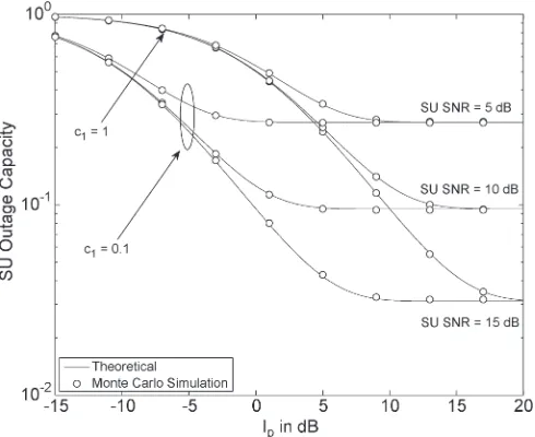
Fig. 2. SU outage capacity, i.e., Pr(SU capacity< R)forR= 1, versus peak interference power for different values ofc1and SU SNR.
Note that, when Ip is very large, the average BER sim-plifies to
Pb=a 2
1−
bλssPm bλssPm+ 2σ2
(58)
where the second term in (57) simplifies usinge−Ip/λspPm →0
as Ip→ ∞. The third term in (57) containing the Gaussian
Q-function vanishes for large Ip. This can be seen by substituting the asymptotic result Q(√T)∼(2πT)−1e−T /2 for largeT[25, eq. (7.1.23)] in (57) and simplifying.
V. NUMERICAL ANDSIMULATIONRESULTS
In this section, we confirm the analytical results derived in Sections III and IV through comparison with Monte Carlo simulations. In the following results, we setσ2= 1,Pm= 1,
Pp= 1 and consider a unit bandwidth B= 1. The PU and SU SNRs are given byPpλpp/σ2andPmλss/σ2, respectively. Moreover, it is assumed that the PU SNR is given by 5 dB. The parameters c1 and c2 are defined by c1=λsp/λss and
c2=Ip/(Ppλpp/σ2). Hence, c1 is the ratio of the SU–PU to the SU–SU link strength, which is usually less than 1 in the common scenario of long PU links and short SU links. Parameter c2 is a proportionality factor so that the acceptable interference Ip is c2 times the PU SNR, and c2<1. Note that the parameterization involving c1 and c2 is more com-pact and allows the system to be defined in terms of relative powers.
We start by comparing the theoretical and simulated cdfs of the RV τ. For this purpose, we have plotted the SU outage capacity in Fig. 2. For a given target transmission rateR, the SU outage capacityP0 can be obtained from the cdf of τ as follows:
P0= Pr
log2
1 + Ptgss
σ2
< R
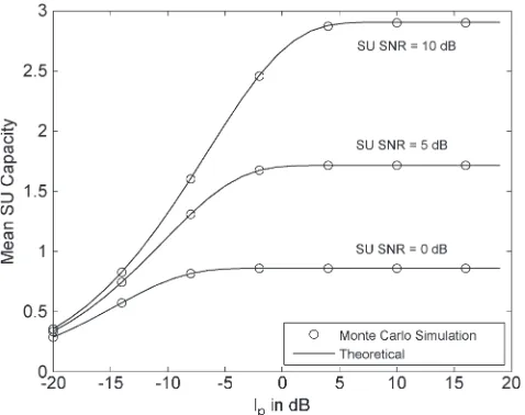
Fig. 3. SU mean capacity versus peak interference power for different values of SU SNR andc1= 0.1.
since σ2= 1. The six curves in Fig. 2 correspond to two different values of c1 and R= 1. The theoretical outage ca-pacities obtained using (12) perfectly match the simulated results.
Fig. 3 shows the mean capacity of the SU (in bits per second per hertz) against Ip under the instantaneous peak received-power constraint and SU transmit received-power constraint. The value of c1 is 0.1, and the PU–SU interference is assumed to be negligible. As expected, the SU capacity is low when the maximum received power at the PU is small since the Ip
constraint limits the SU transmit power. However, as we see, the capacity increases as Ip is increased, and in the high Ip
regime, i.e., Ip>5 dB, the capacity approaches a plateau.
In this region, the maximum transmit power of the SU, i.e.,
Pm, largely dominates (2). Furthermore, as the SU SNR is
increased, a higher capacity can be obtained. This observation is also intuitive. The theoretical results from (20) are perfectly verified by computer simulations.
Under a peak received-power constraint, with the SU trans-mitter employing partial CSI, at times, the actual interference caused to the PU receiver exceeds the level of Ip. This is not acceptable from the PU point of view, and a possible solution is to demand a newIp˜ < Ip. In Fig. 4, we show the resulting percentage capacity loss of the SU againstρdue to such a demand. Calculation of Ip˜ follows the procedure in Section III-B withc1= 0.1, SU SNR= 5dB, and a target of 5% for interference aboveIp. This means that the interference
is allowed to exceedIpfor at most 5% of the time. The capacity
loss for the SU is defined as
CLoss=
COriginal−CNew
COriginal
(60)
whereCOriginalandCNeware the mean SU capacities obtained by substituting Ip and Ip˜ into (20), respectively. When the error in the SU–PU channel estimate is high, i.e., for a small
[image:9.594.44.283.68.257.2]ρ and c2= 0.1, the capacity loss is roughly 65%. However, whenρincreases, the capacity loss becomes insignificant. For example, whenρ= 0.99, it is less than 2% for all three values
[image:9.594.306.546.294.481.2]Fig. 4. Percentage SU capacity loss versus correlation coefficient for different values ofc2,c1= 0.1, and an SU SNR of 5 dB.
Fig. 5. SU mean capacity versus peak interference power for different values of SU SNR,λps= 1, andc1= 0.1.
of c2. Interestingly, no capacity loss is observed forc2= 0.3. In this scenario, the SU is allowed a considerable amount of interference and is mainly restricted by its transmit power. Hence, the channel uncertainty has virtually no effect. Fig. 4 is also useful to determine the accuracy of channel knowledge required at the SU to reap the capacity gains offered by the shared spectrum concept.
In Fig. 5, we compare the SU mean capacities (in bits per second per hertz) against Ip (in decibels) with the primary interference at the SU receiver governed by the parameter
λps= 1. With this level of interference, we observe that the peak capacities are reduced by around 20% compared with Fig. 3, with a larger percentage reduction at lower SU SNR values. Furthermore, in the interference case, higherIpvalues are required before the peak capacities are achieved.
Fig. 6. Theoretical and simulated cdfs of the interference at the primary with quantized CSI and different values ofc1. The system is defined by
[image:10.594.53.285.68.257.2]256 quantization levels,ρ= 0.9,c2= 0.5, and an SU SNR of 5 dB.
Fig. 7. Equivalent correlationρ˜againstρfor SU SNR= 5dB,c1= 0.1, and
c2= 0.5.
Pr(ˆgsp> TN−1) = 10−5. It can be seen that the cdf curves obtained by using the equivalent correlation ρ˜ in (31) match extremely well with the exact simulated curves. This confirms that the equivalentρ˜is a convenient parameter for studying the impact of CSI quantization on the SU mean capacity. Results (not shown here) for different numbers of quantization levels also showed a good match. Fig. 7 shows how the equivalent correlation ρ˜ varies against ρ for four different quantization levels. An appreciable difference between the cases of eight and 16 levels can be observed. However, the difference betweenρ˜
andρis small for the cases of 32 and 256 levels. Hence, for the considered parameters, CSI feedback using 32 levels (5 bits) is sufficient to obtain the capacity gains.
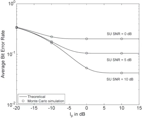
[image:10.594.311.550.306.505.2]Fig. 8 shows the average BER performance using BPSK modulation and assuming that the PU–SU interference is neg-ligible. These results are the counterpart of the mean capacity results shown in Fig. 3. Simulated results have also been plotted to verify the correctness of our analysis. As expected, when
Fig. 8. Average BER versus peak interference power for different SU SNRs with BPSK modulation andc1= 0.1.
Fig. 9. Average BER versus the peak interference power for different SU SNRs with BPSK modulation,λps= 1, andc1= 0.1.
the SU SNR increases, the error performance is improved. However, in all cases, an error floor can be observed. For very low values ofIp, the CR transmit power is very low, resulting
in a large error rate. In fact, in (57), when Ip tends to zero,
the BER is 1/2 for BPSK. WhenIpis large (and, consequently, Ip/gˆsp is larger thanPt), the CR transmitter is constrained to
choose the minimum value, which is its maximum power. This results in a BER floor that can only be lowered by increasing the maximum transmit power of the CR transmitter. Note that the corresponding mean SU capacity results in Fig. 3 also follow the same pattern. It is interesting that the BER curves begin to lift off the floor at about the sameIpvalue as the capacity curves begin to drop off the plateau.
Finally, in Fig. 9, we consider BPSK modulation and com-pare the average BER performance of the secondary system with the primary interference λps= 1, different SU SNRs,
[image:10.594.50.287.311.502.2]We note that all the results in this paper are considered for a single SU and a single PU. The multiple PU case is a reasonably straightforward extension. Here, the SU is required to satisfy theIpconstraint at each PU, and thus, the constraint applied to the maximum interfering path and order statistics can be used for analysis of the SU transmit power. For capacity and BER analysis, the SU receiver is now receiving a sum of interference terms from the PUs. Hence, the analysis is similar in nature, but the details are more complicated. Specifically, the exponential SU–PU channel gain is replaced by the max-imum of several exponentials of different mean values, and the exponential PU–SU interference is replaced by a sum of exponentials with different mean values. The multiple SU case is harder to develop since there are many scenarios here. If the SUs cooperate, then the problem is made more complex since the interference limits can be met by coordinated transmission from the SUs. In the case of full cooperation among the transmitters, the multiple SU system can be treated as a single MIMO broadcast channel. If the SUs independently operate, then each SU can be allocated a portion of the interference constraint, and the transmit power problem is the same as that studied here. However, for performance analysis, there is now interference from both the PU and the other SUs. Hence, again, we have the issue where the exponential PU–SU interference is replaced by a sum of exponentials with different mean values.
VI. CONCLUSION
In this paper, we have studied the SU mean capacity of a spectrum-sharing system. In contrast to most of the existing literature, we have investigated the impact of imperfect channel knowledge of the primary–secondary link on the SU mean capacity under a peak power constraint at the primary receiver. In particular, we have derived the SU mean capacity in closed form. For this situation, when the primary–secondary link gain is incorrectly measured, the inference at the primary receiver can exceed the maximum allowable limit. One method of addressing this issue is to apply a modified lower interference limit so that the original limit is only exceeded with a certain probability. To quantify the loss in applying this reduced limit, we derived the interference cdf in closed form. Additionally, we also considered the impact of quantizing the imperfect CSI with a finite number of quantization levels. It was shown that the quantization effects can also be incorporated into the simple flexible CSI model considered. To this end, we proposed an approximate correlation coefficient to mimic the quantization of the CSI. The accuracy of this simple yet useful approach was confirmed from simulations. To investigate the SU error per-formance, a closed-form average BER expression was derived. Using this result, the error performance for a wide class of modulation schemes can be obtained. In many cases, analytical results have also been considered under various limiting sce-narios, such as high transmit power or high interference limits, which lead to simplified closed-form results.
We are considering the extension of this work to include multiple SUs. It would be extremely cumbersome to develop a completely analytical approach to consider the impact of
multiple SUs. One area that we are investigating is to model the multiple SUs as a global single SU in so far as the interfer-ence to the primary receiver is concerned and then derive SU capacity using the approach given in this paper. In this case, the SU capacity will then be the sum capacity.
REFERENCES
[1] J. Mitola, III, “Cognitive radio: An integrated agent architecture for software defined radio,” Ph.D. dissertation, KTH Roy. Inst. Technol., Stockholm, Sweden, May, 2000.
[2] T. A. Weiss and F. K. Jondral, “Spectrum pooling: An innovative strat-egy for the enhancement of spectrum efficiency,”IEEE Commun. Mag., vol. 42, no. 3, pp. S8–S14, Mar. 2004.
[3] I. F. Akyildiz, W.-Y. Lee, M. C. Vuran, and S. Mohanty, “Next generation/dynamic spectrum access/cognitive radio wireless networks: A survey,”Comput. Netw., vol. 50, no. 13, pp. 2127–2159, Sep. 2006. [4] J. M. Peha, “Approaches to spectrum sharing,”IEEE Commun. Mag.,
vol. 43, no. 2, pp. 10–12, Feb. 2005.
[5] A. J. Goldsmith, S. A. Jafar, I. Maric, and S. Srinivasa, “Breaking spec-trum gridlock with cognitive radios: An information theoretic perspec-tive,”Proc. IEEE, vol. 97, no. 5, pp. 894–914, May 2009.
[6] A. Giorgetti, M. Varrella, and M. Chiani, “Analysis and performance comparison of different cognitive radio algorithms,” in Proc. 2nd Int. Workshop CogART, Aalborg, Denmark, May 2009, pp. 127–131. [7] R. Zhang, “On peak versus average interference power constraints for
spectrum sharing in cognitive radio networks,” inProc. IEEE DySPAN, Chicago, IL, Oct. 2008, pp. 1–5.
[8] M. Gastpar, “On capacity under received-signal constraints,” inProc. 42nd Annu. Allerton Conf. Commun., Control, Comput., Monticello, IL, Sep./Oct. 2004, pp. 1322–1331.
[9] A. Ghasemi and E. S. Sousa, “Fundamental limits of spectrum-sharing in fading environments,”IEEE Trans. Wireless Commun., vol. 6, no. 2, pp. 649–658, Feb. 2007.
[10] L. Musavian and S. Aissa, “Capacity and power allocation for spectrum-sharing communications in fading channels,”IEEE Trans. Wireless Com-mun., vol. 8, no. 1, pp. 148–156, Jan. 2009.
[11] X. Kang, Y.-C. Liang, A. Nallanathan, H. K. Garg, and R. Zhang, “Op-timal power allocation for fading channels in cognitive radio networks: Ergodic capacity and outage capacity,”IEEE Trans. Wireless Commun., vol. 8, no. 2, pp. 940–950, Feb. 2009.
[12] S. A. Jafar and S. Srinivasa, “Capacity limits of cognitive radio with distributed and dynamic spectral activity,”IEEE J. Sel. Areas Commun., vol. 25, no. 3, pp. 529–537, Apr. 2007.
[13] H. A. Suraweera, J. Gao, P. J. Smith, M. Shafi, and M. Faulkner, “Channel capacity limits of cognitive radio in asymmetric fading environments,” in Proc. IEEE ICC, Beijing, China, May 2008, pp. 4048–4053.
[14] C.-X. Wang, X. Hong, H.-H. Chen, and J. Thompson, “On capac-ity of cognitive radio networks with average interference power con-straints,”IEEE Trans. Wireless Commun., vol. 8, no. 4, pp. 1620–1625, Apr. 2009.
[15] P. Popovski, Z. Utkovski, and R. Di Taranto, “Outage margin and power constraints in cognitive radio with multiple antennas,” in Proc. IEEE SPAWC, Perugia, Italy, Jun. 2009, pp. 111–115.
[16] L. Musavian and S. Aissa, “Fundamental capacity limits of spectrum-sharing channels with imperfect feedback,” inProc. IEEE GLOBECOM, Washington, DC, Nov. 2007, pp. 1385–1389.
[17] A. Jovicic and P. Viswanath, “Cognitive radio: An information-theoretic perspective,” IEEE Trans. Inf. Theory, vol. 55, no. 9, pp. 3945–3958, Sep. 2009.
[18] K. S. Ahn and R. W. Heath, Jr., “Performance analysis of maximum ratio combining with imperfect channel estimation in the presence of cochannel interferences,”IEEE Trans. Wireless Commun., vol. 8, no. 3, pp. 1080– 1085, Mar. 2009.
[19] T. L. Marzetta, “BLAST training: Estimating channel characteristics for high capacity space–time wireless,” inProc. 37th Annu. Allerton Conf. Commun., Control, Comput., Monticello, IL, Sep. 1999, pp. 958–966. [20] Q. Sun, D. C. Cox, H. C. Huang, and A. Lozano, “Estimation of
continu-ous flat fading MIMO channels,”IEEE Trans. Wireless Commun., vol. 1, no. 4, pp. 549–553, Oct. 2002.
[22] A. H. Nuttall, “Some integrals involving theQ-function,” Naval Under-water Syst. Cent., New London, CT, Tech. Rep. 4297, Apr. 1972. [23] I. S. Gradshteyn and I. M. Ryzhik,Table of Integrals, Series and Products,
6th ed. San Diego, CA: Academic, 2000.
[24] L. R. Rabiner and R. W. Schafer,Digital Processing of Speech Signals. Englewood Cliffs, NJ: Prentice-Hall, 1978.
[25] M. Abramowitz and I. A. Stegun,Handbook of Mathematical Func-tions With Formulas, Graphs, and Mathematical Tables. New York: Dover, 1964.
Himal A. Suraweera (M’07) was born in Kurunegala, Sri Lanka. He received the B.Sc. degree (with first-class honors) in electrical and electronics engineering from Peradeniya University, Peradeniya, Sri Lanka, in 2001 and the Ph.D. degree from Monash University, Melbourne, Australia, in 2007.
From 2001 to 2002, he was with the Department of Electrical and Electronics Engineering, Peradeniya University, as an Instructor. From October 2006 to January 2007, he was a Research Associate with Monash University. From February 2007 to June 2009, he was with the Center for Telecommunications and Microelectronics, Victoria University, Melbourne, as a Research Fellow. Since July 2009, he has been a Research Fellow with the Department of Electrical and Computer Engineering, National University of Singapore, Singapore. His main research interests include wireless relay networks, cognitive radio, and orthogonal frequency division multiplexing.
Dr. Suraweera serves as a Technical Program Committee Member for in-ternational conferences such as the 2010 IEEE Inin-ternational Conference on Communications, the 2010 IEEE Global Telecommunications Conference, and the 2010 IEEE Wireless Communications and Networking Conference. He was the recipient of the International Postgraduate Research Scholarship from the Australian Commonwealth during 2003–2006, the 2007 Mollie Holman Doctoral and 2007 Kenneth Hunt Medals for his doctoral thesis upon gradu-ating from Monash University, and the IEEE COMMUNICATIONSLETTERS
exemplary reviewer certificate for 2009.
Peter J. Smith(SM’03) received the B.Sc. degree in mathematics and the Ph.D. degree in statistics from the University of London, London, U.K., in 1983 and 1988, respectively.
From 1983 to 1986, he was with the Telecommu-nications Laboratories, GEC Hirst Research Centre. From 1988 to 2001, he was a Lecturer in statistics with Victoria University, Wellington, New Zealand. Since 2001, he has been a Senior Lecturer and Asso-ciate Professor of electrical and computer engineer-ing with the University of Canterbury, Christchurch, New Zealand. His research interests include the statistical aspects of de-sign, modeling, and analysis for communication systems, particularly antenna arrays, multiple-input–multiple-output, cognitive radio, and relays.
Mansoor Shafi(F’93) received the B.Sc.(Eng.) de-gree in electrical engineering from Engineering Uni-versity, Lahore, Pakistan, in 1970 and the Ph.D. degree from the University of Auckland, Auckland, New Zealand, in 1979.
From 1975 to 1979, he was a Junior Lecturer with the University of Auckland. Since 1979, he has been with Telecom New Zealand, Wellington, New Zealand, where he is currently a Principal Advisor (Wireless Systems). His role is to advise Telecom management on the future directions of wireless technologies and standards. He is also an Adjunct Professor with the University of Canterbury, Christchurch, New Zealand. He has widely published in IEEE journals and conference proceedings in the areas of radio propagation, signal processing, multiple-input–multiple-output (MIMO) systems, and adap-tive equalization. His research interests are in wireless communications.