Construction of Global Weak Entropy Solution of Initial Boundary Value Problem for Scalar Conservation Laws with Weak Discontinuous Flux

http://www.scirp.org/journal/ajcm ISSN Online: 2161-1211

ISSN Print: 2161-1203

DOI: 10.4236/ajcm.2017.74033 Dec. 14, 2017 451 American Journal of Computational Mathematics

Construction of Global Weak Entropy Solution

of Initial-Boundary Value Problem for

Scalar Conservation Laws with Weak

Discontinuous Flux

Yihong Dai

1*

, Jing Zhang

2

1_{Department of Mathematics, Jinan University, Guangzhou, China}

2_{Department of Optoelectronic Engineering, Jinan University, Guangzhou, China}

Abstract

This paper is concerned with the initial-boundary value problem of scalar conservation laws with weak discontinuous flux, whose initial data are a func-tion with two pieces of constant and whose boundary data are a constant function. Under the condition that the flux function has a finite number of weak discontinuous points, by using the structure of weak entropy solution of the corresponding initial value problem and the boundary entropy condition developed by Bardos-Leroux-Nedelec, we give a construction method to the global weak entropy solution for this initial-boundary value problem, and by investigating the interaction of elementary waves and the boundary, we clarify the geometric structure and the behavior of boundary for the weak entropy solution.

Keywords

Scalar Conservation Laws with Weak Discontinuous Flux, Initial-Boundary Value Problem, Elementary Wave, Interaction, Structure of Global Weak Entropy Solution

1. Introduction

Consider the following initial-boundary value problem for scalar conservation laws:

( )

( )

( )

( )

0

( )

0, 0, 0

,0 , 0

0, , 0,

t x

b

u f u x t

u x u x x

u t u t t

+ = > >



 _{= >}



 _{= >}



(1)

How to cite this paper: Dai, Y.H. and Zhang, J. (2017) Construction of Global Weak Entropy Solution of Initial-Boundary Value Problem for Scalar Conservation Laws with Weak Discontinuous Flux. American Journal of Computational Ma-thematics, 7, 451-468.

https://doi.org/10.4236/ajcm.2017.74033 Received: October 19, 2017

Accepted: December 11, 2017 Published: December 14, 2017

Copyright © 2017 by authors and Scientific Research Publishing Inc. This work is licensed under the Creative Commons Attribution International License (CC BY 4.0).

http://creativecommons.org/licenses/by/4.0/

DOI: 10.4236/ajcm.2017.74033 452 American Journal of Computational Mathematics where u0

( )

⋅ and ub

( )

⋅ are two bounded and local bounded variation

functions on

[

0,+∞

)

, and the flux f is assumed to be locally Lipschitz continuous.

The initial-boundary value problem for scalar conservation laws plays an important role in mathematical modelling and simulation of practical problem of the one-dimensional sedimentation processes and traffic flow on highways [1] [2][3][4][5]. The existence and uniqueness of global weak entropy solution in the BV-setting were first established by Bardos-Leroux-Nedelec [6] for the initial-boundary value problem of scalar conservation laws with several space variables by vanishing viscosity method and by Kruzkovs method [7], respectively. The core of studying the initial-boundary value problem of conservation laws is the boundary entropy condition which requires only that the boundary data and the boundary value of solution satisfy an inequality. This makes it very interesting to study the initial-boundary value problems of hyperbolic conservation laws. The interested reader is referred to [8]-[14] about other results of existence and uniqueness for the initial-boundary value problem of scalar conservation laws. For the initial-boundary value problem of systems of conservation laws, some progresses have been made in the past: Dubotis-Le Floch

[10] discussed the boundary entropy condition, the authors in [15][16][17][18]

studied the boundary layers, Chen-Frid [19] proved the existence of global weak entropy solution for the system of isentropic gas dynamics equations by using the method of Compensated compactness and vanishing viscosity.

For the geometric structure and regularity and large time behavior of solution of the initial value problem for scalar conservation laws, see [20][21][22] [23] [24][25] etc. Due to the occurrence of boundary, the geometric structure of the solution of (1) is much more difficult than that of corresponding initial value problem. In recent years, for the case of the flux function belonging to C2_-

DOI: 10.4236/ajcm.2017.74033 453 American Journal of Computational Mathematics laws.

The purpose of our present paper is devoted to constructing the global weak entropy solution of the initial-boundary value problem (1) for scalar conservation laws with two pieces of constant initial data and constant boundary data under the condition that the flux function has a finite number of weak discontinuous points, and clarifying the geometric structure and the behavior of boundary for the weak entropy solution.

The present paper is organized as follows. In Section 2, we introduce the definition of weak entropy solution and the boundary entropy condition for the initial-boundary value problem (1), and give a lemma to be used to construct the piecewise smooth solution of (1). In Section 3, basing on the analysis method in

[27], we use the lemma on piecewise smooth solution given in Section 2 to construct the global weak entropy solution of the initial-boundary value problem (1) with two pieces of constant initial data and constant boundary data under the condition that the flux function has a finite number of weak discontinuous points, and state the geometric structure and the behavior of boundary for the weak entropy solution.

2. Definition of Weak Entropy Solution and Related Lemmas

In mathematics, a weak solution (also called a generalized solution) to an ordinary or partial differential equation is a function for which the derivatives may not all exist but which is nonetheless deemed to satisfy the equation in some precisely defined sense. There are many different definitions of weak solution, appropriate for different classes of equations. About the definition of weak solution for the equation of scalar conservation laws, see [31]. Generally speaking, there is no uniqueness for the weak solution of scalar conservation laws. Since the equation of scalar conservation laws arises in the physical sciences, we must have some mechanism to pick out the physically relevant solution. Thus, we are led to impose an a-priori condition on solutions which distinguishes the correct one from the others. The correct one is called the weak entropy solution. Following the papers [3][6][10][12], we give the definition of weak entropy solution of the initial boundary value problem (1).

Definition 1. A bounded and local bounded variable function u x t

( )

, on

[

0,∞ ×

)

[

0,∞

)

is called a weak entropy solution of the initial-boundary problems (1), if for each k∈ −∞ ∞

(

,

)

, and for any nonnegative test function

[

)

[

)

(

)

0 0, 0,

C

φ_∈ ∞ _{∞ × ∞ , it satisfies the following inequality}

(

) ( )

(

( )

)

( )

( )

( )

(

)

(

(

( )

)

( )

)

( )

0 0 0 0

0

d d

, 0 d

0, 0, d 0,

t x

b

u k sgn u k f u f k x t

u x k x x

sgn u t k f u t f k t t

φ φ

φ

φ ∞ ∞

∞

∞

 − + − − 

 

+ −

+ − − ≥

∫ ∫

∫

∫

(2)

DOI: 10.4236/ajcm.2017.74033 454 American Journal of Computational Mathematics

( )

1, 0

1, 0

x sgn x

x

≥ 

= _{− <}



For the initial-boundary value problems (1) whose initial data and bounded data are general bounded variation functions, the existence and uniqueness of the global weak entropy solution in the sense of (2) has been obtained, and the global weak entropy solution satisfies the following boundary entropy condition (3) (see [3][6][10][12]).

Lemma 1. If u x t

( )

, is a weak entropy solution of (1), then,

(

)

( )

(

(

(

)

)

)

( )

(

) ( )

(

)

(

)

0 ,

0 , or 0,

0 ,

0 , , , 0 , , . . 0,

b

b

f u t f k u t u t

u t k

k I u t u t k u t a e t

+ −

+ = ≤

+ −

∈ + ≠ + ≥

(3)

where I u

(

(

0 , ,+t u t

) ( )

_b

)

=_min

{

u

(

0 , ,+ t u t

) ( )

_b

}

, max

{

u

(

0 , ,+ t u t

) ( )

_b

}

_.

In what follows, we give a lemma for the piecewise smooth solution to (1), which will be employed to construct the piecewise smooth solution of (1).

Before stating the lemma, we make the following assumptions to the flux f : (A1) f∈C;

(A2) Its derivative function f′ is a piecewise C1-smooth function with a

finite number of discontinuous points ud_i, and there exist f±′

( )

ud_i such that

( )

di

( )

di

f₋′ u < f₊′ u , where f₋′ and f₊′ represent the left and right derivatives

of f respectively;

(A3) f′′

( )

u >0, u≠ud_i.

Lemma 2. Under the assumptions (A1)-(A3), a piecewise smooth function

( )

,

u x t with piecewise smooth discontinuity curves is a weak entropy solution of (1) in the sense of (2), if and only if the following conditions are satisfied:

(1) u x t

( )

, satisfies Equation (1)₁ on its smooth domains;

(2) If x=x t

( )

is a weak discontinuity of u x t

( )

, , then when u x t t

(

( )

,

)

is

not the discontinuous point of f′, then d

(

(

( )

,

)

)

d

x

f u x t t

t = ′ and when

( )

(

,

)

u x t t is the discontinuous point of f′,

( )

(

)

(

)

(

(

( )

)

)

d d

, or , ;

d d

x x

f u x t t f u x t t

t = −′ t = +′

If x=x t

( )

is a strong discontinuity of u x t

( )

, , then the Rankine-Hugoniot

discontinuity condition

( )

( )

( )

d d

x t f u f u

t u u

− +

− +

− =

− (4)

and the Oleinik entropy condition

( )

( )

( )

( )

f u f u f u f u

u u u u

− + −

− + −

− −

≤

− − (5)

hold, where u±=u x t

(

( )

±0,t

)

, and u is any number between u− and u+;

DOI: 10.4236/ajcm.2017.74033 455 American Journal of Computational Mathematics (4) u x

( )

,0 =u0

( )

x a e x . . ≥0.

Lemma 2 is easily to be proved by Definition 1 and Lemma 1 (see [12][32]). Notations. For the convenience of our construction work, we introduce some notations. Let R u u

(

−, +;

( )

a b,

)

denote a rarefaction wave connecting u− and u₊ from the left to the right centered at point

( )

a b, in the x−t plane, abbreviated as R u u

(

₋, ₊

)

, and S u u

(

−, +;

( )

a b,

)

denote a shock wave x=x t

( )

connecting u₋ and u₊ from the left to the right starting at point

( )

a b, in the

x−t plane, abbreviated as S u u

(

₋, ₊

)

, whose speed x t′

( )

is also denoted by

(

,

)

s u u_{− +} , i.e., x t

( ) (

s u u,

)

f u

( )

f u

( )

,

u u

− +

− +

− +

−

′ = =

− where x=x t

( )

satisfies the Rankine-Hugoniot condition (4) and the Oleinik entropy condition (5).

It is well known that the solution of the shock wave S u u

(

₋, ₊

)

centered at point

( )

a b, and the solution of the central rarefaction wave R u u

(

₋, ₊

)

starting at point

( )

a b, in the x−t plane are respectively expressed as:

( )

( )

( )( )

( )

( )( )

,

,

,

f u f u

u x a t b

u u u x t

f u f u

u x a t b

u u

− +

−

− +

− +

+

− +

− 

< + −

 ₋

 = 

−

 _{> + −}

 ₋

 and

( )

( )(

)

( )

( )(

)

( )(

)

( )(

)

1 ,

, ,

,

u x a f u t b

x a

u x t f a f u t b x a f u t b

t b

u x a f u t b

− −

−

− +

+ +

′

 < + −

 ₋

 _′   _{′ ′}

= _{ −} _ + − < < + −



 > + ′ −

 where t>b.

3. Construction of Global Weak Entropy Solutions

In this section, with the aid of the analysis method in [27], the authors in [27]

used the truncation method to construct the global weak entropy solution

( )

,

u x t of initial-boundary value problem for scalar conservation laws with C2_{-smooth flux function. This analysis method is basing on the tracing of the}

position of elementary waves (especially the shock wave) in the weak entropy solution v x t

( )

, for the corresponding initial value problem and the boundary

entropy condition (3). According to [27], if v x t

( )

, does not include any shock

wave or includes a shock wave whose position is not the following case: the shock wave lies in the second quadrant and the sign of the shock speed is changed from negative to positive before a finite time, then

( ) ( )

, , _{0, 0}

x t

u x t =v x t _{> >} ;

otherwise we need to find some time t=t0 and construct the local solution to

this time, and then take the time t=t0 as the new initial time to extend this

DOI: 10.4236/ajcm.2017.74033 456 American Journal of Computational Mathematics corresponding initial value problem. Moreover, we will also describe the interaction of elementary waves with the boundary and clarify the behaviors of the global weak entropy solution near the boundary.

Consider the following initial-boundary problem:

( )

( )

( )

0, 0, 0

, 0 ,0

,

0, , 0

t x

m

u f u x t

u x a

u x

u x a

u t u t

+

−

 + = > >

 _{< <}



 ₌

  _>

 

 _{≡ >}



(6)

where u u±, m are constant, for x>0 and x≠a a, >0 is a constant. We first

consider the case that f has only one weak discontinuous point, and then the case that f has finitely many weak discontinuities.

3.1. The Case That

f

Has Only One Weak Discontinuous Point

Throughout this sub-section, the flux f is assumed to satisfy (A₁) and the following conditions:

(A2)' f′ is a piecewise C1—smooth function with one weak discontinuous

point ud, and there exist f±′

( )

ud such that f−′

( )

ud < f+′

( )

ud ;

(A3)' f′′

( )

u >0, u≠ud.

We first discuss the initial boundary value problem (6) for the case of

m

u =u+≠u−, which is called Riemann initial-boundary problem, written as

( )

( )

( )

0, 0, 0

,0 , 0

0, , 0,

t x

u f u x t

u x u x

u t u t

+

−

+ = > > 

 _{≡ >}



 _{≡ >}



(7)

where u₋≠u₊. And then investigate (6) with u_m ≠u+. For definiteness, it has

no harm to assume that f

( )

0 = f

( )

0 ′=0 and ud<0 in this sub-section. The

other cases can be dealt with similarly.

3.1.1. Riemann Initial-Boundary Problem

When

(

u₋−u_d

) (

⋅ u₊−u_d

)

≥0, (7) is degenerated into a corresponding problem

with 2

f∈C (see [27]). We now construct the weak entropy solution of (7) only for the case of

(

u−−ud

) (

⋅ u+−ud

)

<0. We divide our problem into two

cases: (1) u−<ud<u+; (2) u+<ud<u−.

Case (1) u−<ud<u+.

Consider the following Riemann problem corresponding to (7):

( )

( )

0

( )

0, , 0

, 0

,0 :

, 0.

t x

v f v x t

u x

v x v x

u x

−

+

+ = − ∞ < < ∞ >



 _<



 ₌

= 

 _>

 

(8)

In this case, since the flux function has a weak discontinuity point u=ud, the

Riemann problem (8) includes only a rarefaction wave R=R u u

(

−, d

)

R u u

(

d, +

)

DOI: 10.4236/ajcm.2017.74033 457 American Journal of Computational Mathematics

( )

( )

( )

( )

( )

( )

( )

( )

( )

( )

1 1 , ( ) , , , , , d

d d d

d

u x f u t

x

f f u t x f u t

t

u f u t x f u t

v x t

x

f f u t x f u t

t

u x f u t

− − − − − − + − + + + + ′ <   _{ }

 ′ _{ } ′ ≤ < ′

 _{ }

 _{′ ≤ < ′}

= 

 _{ }

 ′ _{ } ′ ≤ < ′

  

 _{≥ ′}

 Let

( ) ( )

, , _{, 0}

x t

u x t =v x t _> , then u

(

0 ,+t

)

=min

{

u₊,0

}

, hence, it holds the

boundary entropy condition:

(

)

(

)

( )

(

)

(

(

)

(

)

)

0 ,

0 , 0 , , 0 , .

0 ,

f u t f k

k u u t k u t

u t k −

+ −

≤ ∀ ∈_ + _ ≠ +

+ −

It is easy to verify that u x t

( )

, also satisfies all other conditions in Lemma 2.

Therefore, by Lemma 2, u x t

( )

, is the global weak entropy solution of (7).

Case (2) u+<ud<u−.

In this case, (8) includes only a shock wave S u u

(

₋, ₊

)

at point

( )

0,0 in the

x−t plane. This shock wave solution can be expressed as follows:

( )

, ,

(

(

,

)

)

, ,

u x s u u t v x t

u x s u u t

− − +

+ − +

< 

=  _> 

where s u u

(

₋, ₊

)

is the speed of the shock S u u

(

₋, ₊

)

. Let

( ) ( )

, 0

, ,

x t

u x t =v x t _> ,

then

(

0 ,

)

, as

(

(

,

)

)

0

, as , 0

u s u u

u t

u s u u

+ − +

− − +

≤ 

+ =  _>



From Lemma 2, we can easily verify that u x t

( )

, is the global weak entropy

solution of (7).

3.1.2. The General Problem with um ≠u+

Consider the following initial value problem corresponding to (6):

( )

( )

0

( )

0, , 0

, 0

,0 : , 0

, .

t x

m

v f v x t

u x

v x v x u x a

u x a −

+

+ = − ∞ < < ∞ > 

 _<

 

 _{= =} _{< <}

 



 _{ >}



(9)

According to the solution structure of (9), we construct the global weak entropy solution of (6) with um ≠u+ by dividing our problem into five cases:

(1) u−=um ≠u+ ; (2) u−<um<u+ ; (3) u+<um<u− ; (4) u u−, +<um ; (5) ,

m

u <u u− +.

Case (1) u−=um≠u+.

In fact, when u−=um,

(

u−−ud

) (

⋅ u+−ud

)

≥0, (6) becomes a problem with 2

f∈C , which was discussed in [27]. We now investigate the case of

(

u₋−u_d

) (

⋅ u₊−u_d

)

<0. (9) is degenerated into a Riemann problem.

DOI: 10.4236/ajcm.2017.74033 458 American Journal of Computational Mathematics at

( )

a,0 of the x−t plane, appears in the weak entropy solution of (9). This rarefaction wave solution of (9) can be written as:

( )

( )

( )

( )

( )

( )

( )

( )

( )

( )

1

1

,

,

, ,

,

,

d

d d d

d

u x a f u t

x a

f a f u t x a f u t

t

v x t u a f u t x a f u t

x a

f a f u t x a f u t

t u

− −

−

− −

− +

−

+ +

+

′ < + −

 

′ _{ } + ′ ≤ < + ′

 

′ ′

= + ≤ < +

−

 

′ _{ } + ′ ≤ < + ′

 

( )

x a f u+ t.

        

 _{≥ + ′}



Let

( ) ( )

, , _{, 0}

x t

u x t v x t >

= _{, where} v x t

( )

, is the weak entropy solution of (9). It

is easy to verify u x t

( )

, satisfies all conditions in Lemma 2, thus u x t

( )

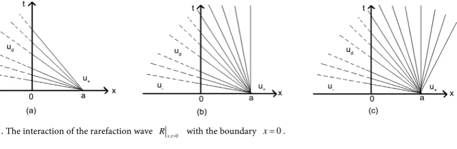
, is the

global weak entropy solution of (6). It includes only a rarefaction wave Rx t,>0 ,

which will interact with the boundary x=0 and be completely absorbed (if 0

u₊≤ ) (see Figure 1(a) and Figure 1(b)) or partially absorbed (if u₊>0) (see

Figure 1(c))by the boundary.

If u−=um>u+, the weak entropy solution v x t

( )

, of (9) includes only a

shock wave emanating at point

( )

a,0 of the x−t plane, which can be expressed as follow:

( )

, ,

(

(

,

)

)

, ,

u x a s u u t v x t

u x a s u u t

− − +

+ − +

< + 

=  _{> +} 

Let

( ) ( )

, , _{, 0}

x t

u x t v x t >

= _{, then by Lemma 2, it is also easy to verify that} u x t

( )

,

is the global weak entropy solution of (6). It includes only a shock wave

( )

(

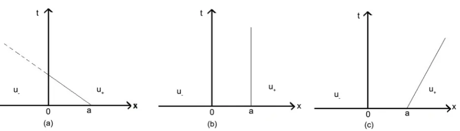
, ; ,0

)

S u u− + a , which will interact with the boundary x=0 and be absorbed

(if s u u

(

₋, ₊

)

≤0) (see Figure 2(a)) or be far away from the boundary (if

(

,

)

0

s u u_{− +} > ) (see Figure 2(b) and Figure 2(c)). Case (2) u−<um<u+.

If u u±, m≥ud, or u u±, m≤ud, (6) becomes a problem with f ∈C2, see [27].

We now consider the following three cases: u−<um<ud <u+, u−<ud <um<u+,

and u−<um =ud <u+.

When u−<um<ud <u+, two rarefaction waves R u u

(

−, m

)

and

(

)

(

)

1 m, d d,

R =R u u R u u₊ , centered at point

( )

0,0 and

( )

a,0 , respectively,

appear in the weak entropy solution v x t

( )

, of (9); when u−<u_d <u_m<u+, [image:8.595.88.535.587.733.2]

[image:9.595.66.534.65.199.2]

DOI: 10.4236/ajcm.2017.74033 459 American Journal of Computational Mathematics Figure 2. The interaction of the shock wave S u u

(

−, +;

( )

a, 0

)

with the boundary x=0.

two rarefaction waves R2 =R u u

(

−, d

)

R u u

(

d, m

)

and R u u

(

m, +

)

, centered at

point

( )

0,0 and

( )

a,0 , respectively, appear in the weak entropy solution

( )

,

v x t of (9); when u−<u_m =u_d <u+ , two centered rarefaction waves

(

, d

)

R u u₋ and R u u

(

d, +

)

, centered at point

( )

0,0 and

( )

a,0 , respectively,

appear in the weak entropy solution v x t

( )

, of (9). The two rarefaction waves in

( )

,

v x t , centered at point

( )

0,0 and

( )

a,0 , respectively, will not overtake each

other since the propagating speed of the wave front in the first wave is not greater than that of the wave back in the second wave. Let

( ) ( )

, , _{, 0}

x t

u x t v x t >

= _,

from Lemma 2, we can easily verify that u x t

( )

, is the global weak entropy

solution of (6).

When u−<um<ud <u+, u x t

( )

, includes only a rarefaction wave Rx t,>0 ,

which will interact with the boundary x=0 and be partially absorbed (if 0

u₊> ) or absorbed (if u₊≤0) by the boundary.

When u−<ud <um<u+, if f′

( )

um =0, u x t

( )

, includes only the central

rarefaction wave R u u

(

_m, ₊

)

far away from the boundary x=0; if f′

( )

u_m >0,

( )

,

u x t includes two central rarefaction waves ₂

, 0 x t

R _> and R u u

(

_m, ₊

)

far away

from the boundary; if f′

( )

u_m <0, u x t

( )

, includes only the central rarefaction

wave R u u

(

m, +

)

_{x t,>0}, which will interact with the boundary and be partially

absorbed (if u₊ >0) or completely absorbed (if u₊≤0) by the boundary.

When u−<um=ud <u+, u x t

( )

, includes only the central rarefaction wave

(

d,

)

_{x t, 0}

R u u+ _> , which will interact with the boundary and be partially absorbed

(if u₊>0) or completely absorbed (if u₊≤0) by the boundary.

Case (3) u+<um<u−.

The discussion for this case is the same as that of the corresponding case in

[27].

Case (4) u u−, +<um.

When u u−, +≥ud, or um≤ud, then (6) is degenerated into the problem with

2

f∈C . When u−≥ud, then the discussion on this problem is the same as that

of the case 2

f ∈C . Hence, we only investigate the case of u−<ud <u um, +<um.

In this case, an initial rarefaction wave R=R u u

(

₋, _d

)

R u u

(

_d, _m

)

centered at

point

( )

0,0 and an initial shock wave S u u

(

_m, ₊

)

starting at point

( )

a,0

DOI: 10.4236/ajcm.2017.74033 460 American Journal of Computational Mathematics

[33], we give the statement of interaction of the initial rarefaction wave R and the initial shock wave S u u

(

_m, ₊

)

. The rarefaction wave R interacts with the

shock wave S u u

(

_m, ₊

)

lying on its right at some finite time t=t₁, and the

shock S u u

(

_m, ₊

)

will cross R after t=t₁. The initial shock wave curve is

denoted as x=x t

( )

, and the resulting shock after the interaction of R and

(

_m,

)

S u u₊ is still denoted as x=x t

( )

, which is regarded as an extension of the original shock x=x t

( )

. The right state of the resulting shock is a constant u₊.

If u₊<u₋, the shock x=x t

( )

will cross the whole of the initial rarefaction wave R completely at some finite time; if u₊=u₋, the shock x=x t

( )

is able to cross the whole of R completely only when t→ ∞; if u₊>u₋, it is impossible

for this shock wave to cross the whole of R completely, but it is able to cross the right part of R: R u u

(

+, m

)

(if u+≥ud ) or R u u

(

+, d

)

R u u

(

d, m

)

(if

d

u−<u+<u ) when t→ ∞. The shock x=x t

( ) (

t>0

)

is a piecewise smooth

curve. First, the shock wave x=x t

( ) (

t>0

)

cross the right part R u u

(

_d, _m

)

of

R with a varying speed of propagation during the penetration. If it is able to cross the whole of R u u

(

_d, _m

)

completely at some finite time, then it crosses the

domain of constant state u=ud with a constant speed of propagation. When

the shock x=x t

( ) (

t>0

)

encounters the rightmost characteristic line of the

rarefaction wave R u u

(

₋, _d

)

, it begins to cross R u u

(

₋, _d

)

with a varying speed

of propagation again. For the position of the shock x=x t

( ) (

t>0

)

, we have

one of the following cases: 1) the shock x=x t

( )

is located in the first quadrant of the x−t plane; 2) the shock x=x t

( )

enters the second quadrant from the first quadrant including the t-axis at some finite time and then keeps staying in the second quadrant. Let

( ) ( )

, , _{, 0}

x t

u x t v x t >

= _{, then by Lemma 2,} u x t

( )

, is the

global weak entropy solution of (6).

We now state the interaction of the elementary and the boundary x=0 for

the global weak entropy solution of (6). When the shock x=x t

( )

in v x t

( )

, is

in the first quadrant of the x−t plane, the elementary wave in the solution

( )

,

u x t of (6) does not interact with the boundary x=0; when the shock wave

( )

x=x t of v x t

( )

, enters the second quadrant from the first quadrant

including the t-axis and then keeps staying in the second quadrant, the shock wave x=x t

( )

in u x t

( )

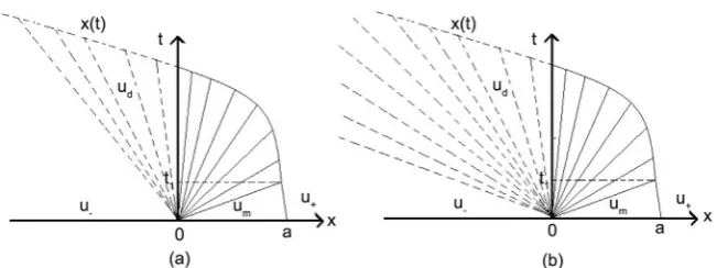
, interacts with the initial rarefaction wave

, 0 x t

R _> on its right at t=t1, and then crosses Rx t,>0 at its right at t>t1, finally it collides

with the boundary x=0 and is absorbed by the boundary (see Figure 3(a) and

Figure 3(b)).

Case (5) um<u u−, +

If u u−, +≤ud, or um≥ud, then (6) becomes a problem with

2

f∈C (see

[27]). If u+≤ud<u−, the discussion of the problem is the same as that of the

case _f∈_C2. We only consider the case of

m d

u <u <u+ in the following

discussion.

In this case, an initial shock wave S u u

(

₋, _m

)

starting at point

( )

0,0 and an

[image:11.595.209.535.66.188.2]

DOI: 10.4236/ajcm.2017.74033 461 American Journal of Computational Mathematics Figure 3. The interaction of the shock wave x=x t

( )

with the boundary x=0.

x−t plane appear in the weak entropy solution v x t

( )

, of (9). We denote this

initial shock wave curve by x=x t

( )

. As in [33], the shock S u u

(

₋, _m

)

interacts

with the rarefaction wave R on its right at some time

t

=

t

1 and at

t

>

t

1, it will

cross R with a varying speed of propagation during the penetration. We denote the generating shock wave still by x=x t

( )

, whose left state is a constant

u

₋. If

u

₋

>

u

₊ , the shock wave x=x t

( )

will completely penetrate the initial rarefaction wave R at a finite time; if

u

₊

=

u

₋, the shock x=x t

( )

is able to cross the whole of R completely only when t→ ∞; if

u

₋

<

u

₊, it is impossible for this shock wave to cross the whole of R completely, but it is able to cross the left part of R: R u u

(

_m, ₋

)

(if u−≤u_d) or R u u

(

m, d

)

R u u

(

d, −

)

(if u−>ud) when

t→ ∞. After

t

=

t

₁, x=x t

( )

will cross the rarefaction waves on its right with a non-decreasing speed. The shock x=x t

( ) (

t>0

)

is a piecewise smooth

curve. During the process of penetrating R=R u u

(

_m, _d

)

R u u

(

_d, ₊

)

, it first

crosses the leftmost part R u u

(

_m, _d

)

of R with a varying speed, and then crosses

the constant state u=ud with constant speed. When the shock wave

( ) (

0

)

x=x t t> encounters the characteristic line of the leftmost characteristic line of the rarefaction wave R u u

(

_d, ₊

)

, it again begins to cross the rarefaction

wave R u u

(

_d, ₊

)

with a varying speed. For the shock x=x t

( ) (

t>0

)

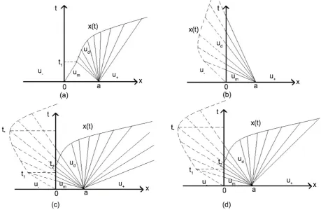
, it holds

one of the following three cases: (a) when the initial shock speed s u u

(

₋, _m

)

≥0,

the shock x=x t

( )

interacts with the initial rarefaction wave R in the first quadrant including the t-axis and keeps staying in the first quadrant after interaction (see Figure 4(a)); (b) when s u u

(

₋, _m

)

<0,u₊< <0 u₋ and

( )

( )

f u₋ ≤ f u₊ , the shock x=x t

( )

interacts with R in the second quadrant and remains in the second quadrant after interaction (see Figure 4(b)); (c) when

(

, _m

)

0

s u u₋ < , if 0≤u₊≤u u₋, ₋≠0 or 0 <u₋≤u₊ or u₊< <0 u₋,

( )

( )

f u₋ > f u₊ , the shock x=x t

( )

crosses the t-axis from the second quadrant at some finite time greater than t1, and then enters the first quadrant,

and keeps staying in the first quadrant after that finite time (see Figure 4(c) and

Figure 4(d)).

In sub-case (a) and (b), let

( ) ( )

, , _{, 0} x t

u x t v x t >

= _{, then from Lemma 2, we can}

verify that u x t

( )

, is the global weak entropy solution of (6). The interaction of

the elementary wave and the boundary x=0 in the solution u x t

( )

, of (6) is

[image:12.595.76.536.73.373.2]

DOI: 10.4236/ajcm.2017.74033 462 American Journal of Computational Mathematics Figure 4. The interaction of the shock wave x=x t

( )

with the boundary x=0.

solution of (6) does not include the interaction of elementary waves and the boundary x=0; when s u u

(

₋, _m

)

=0, the rarefaction wave

(

_m, _d

)

(

_d,

)

R=R u u R u u₊ collides with the boundary x=0 at time t=t₁, and

the boundary x=0 reflects a new shock wave tangent to the boundary itself at

point

( )

0,t1 , which is just the restriction of x=x t

( )

at t>t1 and will

penetrate R after t=t1. For sub-case (b), the weak entropy solution of (6) only

includes the rarefaction wave R=R u u

(

m, d

)

R u u

(

d, +

)

_{x t,>0}, which interacts

with the boundary x=0 at some time and is absorbed completely by the

boundary.

For sub-case (c), there exists u*∈

(

um,0

)

such that f u

( )

* = f u

( )

− .

Furthermore, there is t*>t1 such that

( )

(

(

( )

)

)

*

* * 0, 0

, 0, 0,

0,

t t x t s u u x t t t t

t t −

< < < 



′ = + _= =

> > 

for u*≠ud and there are exist t t*,*>t t1

(

*<t*

)

such that

( )

(

(

( )

)

)

* **

*

0, 0

, 0, 0,

0,

t t

x t s u u x t t t t t

t t

−

< < < 

′ = + _= ≤ ≤

> > 

DOI: 10.4236/ajcm.2017.74033 463 American Journal of Computational Mathematics the weak entropy solution of (9). If we construct the solution of (6) by taking

( ) ( )

, , _{, 0}

x t

u x t v x t >

= _{as in sub-cases (a), (b), then this} u x t

( )

, does not satisfy

the boundary entropy condition (4) for t>t2, where t2 = −a f+′

( )( )

u* <t* is

the time at which the characteristic line with speed f+′

(

u x t

(

( )

* +0,t*

)

)

from

the point

(

x t

( )

* ,t*

)

backward to x-axis intersects the t-axis (see Figure 4(c)

and Figure 4(d)). Thus, by virtue of Lemma 2, it is not the weak entropy solution of (6). We need to reconstruct the solution of (6). Take

(

2

)

(

)

2

, 0 ,

, 0 , 0

u x

v x t

v x t x

− <



=  _{− >}

 (10)

as the new initial value of (9)1, then the solution v x t

( )

, of the initial value

problem (9)1, (10) in

(

0,∞ ×

) (

t2,∞

)

includes only a new shock wave x x

( )

t

+ = starting at point

(

0,t2

)

, whose original speed is zero and the left state is u−.

When t>t2, this shock crosses the rarefaction wave R(x a− )t>f+′( )u_* on its right

with a varying positive speed of propagation in the first quadrant. Let

( )

( )

( )

2

2 , , 0 ,

, , ,

v x t t t V x t

v x t t t

< < 

=  _≥



then, from Lemma 2, this

( )

,

( )

, _{0, 0}

x t

u x t =v x t _{> >} is the global weak entropy solution of (6). Now we give the statement of the interaction of the elementary and the boundary x=0 in the solution u x t

( )

, of (6) (see Figure 4(c) and

Figure 4(d)). For the problem (6), an initial rarefaction wave

(

m, d

)

(

d,

)

R=R u u R u u₊ emanates from the point

( )

a,0 on the x-axis. One

part of R collides with the boundary x=0, and then the boundary x=0

reflects a new shock wave x=x+

( )

t at t=t₂ with zero original speed, which

will penetrate another part R(x a− )t>f+′( )u* of R with a varying positive speed of propagation in the first quadrant. This shock is just that one in v x t

( )

, .

3.2. The Case That

f

Has Finitely Many Weak Discontinuous Points

In this sub-section, the flux f is supposed to satisfy the conditions (A₁)-(A₃). As an example, we discuss the case that f′ has only two discontinuous points, and we can similarly deal with the case that f′ has n discontinuous points. It has no harm to assume that f

( )

0 = f′

( )

0 =0 and

1 2 0

d d

u <u < as in above sub-section.

3.2.1. Riemann Initial-Boundary Problem

We now construct the global weak entropy solution of (7) under the condition that ud1,ud2 are located between u− and u+. If not so, see [27] or sub-Section 3.1.1.

Case (1) u−<ud1,ud2<u+.

In this case, since the flux function f has two weak discontinuous points

1, 2

d d

u u , (8) includes only a rarefaction wave

(

, d1

) (

d1, d2

) (

d2,

)

DOI: 10.4236/ajcm.2017.74033 464 American Journal of Computational Mathematics

( )

( )

( )

( )

( )

( )

( )

( )

( )

( )

( )

( )

( )

1

1 1 1

1 2

2 2 2

1 1 1 , , , , , , , d

d d d

d d

d d d

u x f u t

x

f f u t x f u t

t

u f u t x f u t

x

f f u t x f u t

v x t

t

u f u t x f u t

x f t − − − − − − + − + − − + − ′ <  

′ _{ } ′ ≤ < ′

 

′ ≤ < ′

 

′ ′ ≤ < ′

= _{ }

 

′ ≤ < ′

  ′  _{ }

( )

( )

( )

2 , . d

f u t x f u t

u x f u t

+ + + +             

′ ≤ < ′

 

 _{≥ ′}



Let

( ) ( )

, , _{, 0}

x t

u x t =v x t _> then u

(

0 ,+ t

)

=min

{

u₊,0

}

. It is easy to verify that

( )

,

u x t is the global weak entropy solution of (7). Case (2) u+<ud<u+.

In this case, only a shock wave S u u

(

₋, ₊

)

starting at point

( )

0,0 appears in

the weak entropy solution of (8). This shock wave solution can be denoted as:

( )

, ,

(

(

,

)

)

, ,

u x s u u t v x t

u x s u u t

− − +

+ − +

< 

=  _> 

where s u u

(

₋, ₊

)

is the speed of the shock wave S u u

(

₋, ₊

)

. Let

( ) ( )

, , _{, 0}

x t

u x t =v x t _> , then

(

0 ,

)

, if

(

(

,

)

)

0

, if , 0

u x s u u u t

u x s u u

+ − +

− − +

< ≤



+ =  _{> >}



By Lemma 2, one can verify that u x t

( )

, is the global weak entropy solution

of (7).

3.2.2. The General Problem with um≠u+

For the initial boundary value problem (6) with um≠u+, we only investigate the

case of u_m<u_d1<u_d2 < <0 u u₋, ₊, f u

( )

_m > f u

( )

₋ , which is the most typical and complicated case.

In this case, an initial shock wave S u u

(

₋, _m

)

, emanating at point

( )

0,0 , and

an initial rarefaction wave R=R u u

(

_m, _d1

) (

R u_d1,u_d2

) (

R u_d2,u₊

)

, centered at point

( )

a,0 , appear in the weak entropy solution v x t

( )

, of the corresponding

initial value problem (9). We denote this shock by x=x t

( )

, whose original speed of propagation is negative. The shock x=x t

( )

will interact with the rarefaction wave R on its right at some finite time t=t1. This interaction will

generate a new shock, still denoted by x=x t

( )

. The left state of the resulting shock wave is u₋. If u₋>u₊, the shock x=x t

( )

is able to cross the whole of R at finite time (see Figure 5(a)); if u₋=u₊, the shock x=x t

( )

is able to cross the whole of R completely only when t→ ∞; if u₋<u₊, it is impossible for the

shock to cross the whole of R completely, but it is able to cross the left part

(

m, d1

) (

d1, d2

) (

d2,

)

R=R u u R u u R u u₊ of R at t→ ∞ (see Figure 5(b)). After

1

[image:15.595.90.536.73.221.2]

DOI: 10.4236/ajcm.2017.74033 465 American Journal of Computational Mathematics Figure 5. The interaction of the shock wave x=x t

( )

with the boundary x=0.

non-decreasing speed of propagation. The shock x=x t

( ) (

t>0

)

is a piecewise

smooth curve.

During the process of its penetrating the rarefaction wave R, the shock wave

( ) (

0

)

x=x t t> first crosses the leftmost part

(

)

1 ,

m d

R u u of R with a varying speed of propagation, and then crosses the constant state u=ud₁ with constant

speed. When the shock wave x=x t

( )

encounters the characteristic line of the leftmost characteristic line of the rarefaction wave R u

(

_d1,u_d2

)

, it again begins to cross the rarefaction wave R u

(

d1,ud2

)

with a varying speed. And then it crosses the constant state u=ud₂ with constant speed. Finally, it crosses the

rightmost part R u

(

d2,u−

)

of R with a varying speed of propagation.

In view of um<ud₁<ud₂ < <0 u u−, + and f u

( )

m > f u

( )

− , there exists

(

)

* m,0

u ∈ u such that f u

( )

_* = f u

( )

₋ . Furthermore, there is t_*>t₁ such that

( )

(

(

( )

)

)

* *

* 0, 0

, 0, 0,

0,

t t x t s u u x t t t t

t t −

< < < 



′ = + _= =

> > 

for u*≠ud1,ud2 and there are exist t0*,t*>t t1

(

0*<t*

)

, such that

( )

(

(

( )

)

)

0* 0**

* 0, 0

, 0, 0,

0,

t t x t s u u x t t t t t

t t −

< < < 



′ = + _= ≤ ≤

> > 

for u*=ud1 or ud2 , where x t′

( )

is the speed function of the shock wave

( )

x=x t in the weak entropy solution v x t

( )

, of (9). The position of the shock

( ) (

0

)

x=x t t> is stated as follows: the shock x=x t

( )

lies in the second quadrant of the x−t plane as t∈

(

0,t_**

)

, and cross the t-axis at t=t_**, and

then enter and keep staying in the first quadrant (see Figure 5(a)), where

( )

** *

t >t is the unique time at which the shock x=x t

( )

and the t-axis axes intersect.

In what follows, we construct the global weak entropy solution of (6). Let t2

denote the intersection time of the t-axis and the characteristic line with speed

( )

(

)

(

* 0,*

)

f+′ u x t + t from the point

(

x t

( )

* ,t*

)

backward to x-axis, namely,

( )( )

2 * *

t = −a f₊′ u <t . First take

( ) ( )

, 0

, ,

x t

DOI: 10.4236/ajcm.2017.74033 466 American Journal of Computational Mathematics

( )

,

u x t is the local weak entropy solution of (6) on

(

0,+∞ ×

) (

0,t2

)

. Next we

will extend this u x t

( )

, to

(

0,+∞ ×

) (

0,+∞

)

. Consider the following Cauchy

problem:

( )

( )

(

)

(

)

2

2

2

0, ,

, 0 ,

, 0 , 0

t x

v f v x t t

u x

v x t

v x t x

−

+ = − ∞ < < +∞ > 

 _{ <}

 _{= }

 _{− >}

 

(11)

The weak entropy solution v x t

( )

, of (11) in

(

0,+∞ ×

) (

t₂,+∞

)

includes

only a shock wave x=x+

( )

t starting at

(

0,t2

)

, whose original speed of

propagation is zero. The shock x=x+

( )

t will cross this part of the rarefaction

wave on its right: R₍x a− ₎t>f+′_{( )}u_* with a varying positive speed of propagation

during the penetration in the first quadrant as t>t2. Then by Lemma 2,

( )

( )

2

0,

, : ,

x t t

u x t =v x t _{> >} is the weak entropy solution of (6) on

(

0,+∞ ×

) (

t2,+∞

)

.

Thus we accomplish the construction of the solution to (6) (see Figure 5(b)). The weak entropy solution of (6) has the following geometric structure near the point

(

0,t2

)

: A part of the rarefaction wave

(

m, d1

) (

d1, d2

) (

d2,

)

R=R u u R u u R u u₊ centered at point

( )

a,0 collides with

the boundary x=0, then the boundary reflects a new shock wave tangent to the

boundary x=0 at time t=t₂, which will penetrate another part _{( ) ( )}

*

x a t f u

R

+′ − >

of R with a varying positive speed of propagation in the first quadrant. This shock is just that one in v x t

( )

, .

4. Conclusion

This paper is mainly concerned about the initial-boundary value problem of scalar conservation laws with weak discontinuous flux, whose initial data are a function with two pieces of constant and whose boundary data are a constant function. Under this condition, the flux function has a finite number of weak discontinuous points, by using the structure of weak entropy solution of the corresponding initial value problem and the boundary entropy condition developed by Bardos-Leroux-Nedelec. We give a construction method to the global weak entropy solution for this initial-boundary value problem, and by investigating the interaction of elementary waves and the boundary. We clarify the geometric structure and the behavior of boundary for the weak entropy solution.

Acknowledgements

This work was supported by National Natural Science Foundation of China (No. 11271160).

References

DOI: 10.4236/ajcm.2017.74033 467 American Journal of Computational Mathematics [2] Bustos, M.C., Concha, F. and Wendland. W.L. (1990) Control of Continuous Sedi-mentation of an Ideal Suspension as Initial Boundary Value Problem. Mathematical Methods in the Applied Sciences, 12, 533-548.

https://doi.org/10.1002/mma.1670120607

[3] Bustos, M.C., Paiva, F. and Wendland, W.L. (1996) Entropy Boundary Condition in the Theory of Sedimentation of Ideal Suspension. Mathematical Methods in the Applied Sciences, 19, 679-697.

https://doi.org/10.1002/(SICI)1099-1476(199606)19:9<679::AID-MMA784>3.0.CO; 2-L

[4] Richards, P.I. (1956) Shock Waves on Highways. Operations Research, 4, 42-51. https://doi.org/10.1287/opre.4.1.42

[5] Whitham, G.B. (1974) Linear and Nonlinear Waves. Wiley-Interscience, New York. [6] Bardos, C., Leroux, A.Y. and Nedelec, J.C. (1979) First Order Quasilinear Equations

with Boundary Conditions. Communications in Partial Differential Equations, 4, 1017-1034. https://doi.org/10.1080/03605307908820117

[7] Kruzkov, S.N. (1970) First Order Quasilinear Equations in Several Independent Va-riables. Mathematics of the USSR-Sbornik, 10, 217-243.

https://doi.org/10.1070/SM1970v010n02ABEH002156

[8] Szepessy, A. (1989) Measure-Value Solution to Scalar Conservation Laws with Boundary Conditions. Archive for Rational Mechanics and Analysis, 139, 181-193. https://doi.org/10.1007/BF00286499

[9] Joseph, K.T. (1989) Burgers Equation in the Quarter Plane: A Formula for the Weak Limit. Communications on Pure and Applied Mathematics, 41, 133-149.

https://doi.org/10.1002/cpa.3160410202

[10] Dubotis, F. and LeFloch, P.G. (1988) Boundary Conditions for Nonlinear Hyper-bolic System of Conservation Laws. Differential Equation, 8, 93-122.

https://doi.org/10.1016/0022-0396(88)90040-X

[11] LeFloch, P.G. and Nedelec, J.C. (1988) Explicit Formula for Weighted Scalar Non-linear Conservation Laws. Transactions of the American Mathematical Society, 308, 667-683. https://doi.org/10.1090/S0002-9947-1988-0951622-X

[12] Pan, T. and Lin, L.W. (1995) The Global Solution of the Scalar Nonconvex Conser-vation Laws with Boundary Condition. Journal of Partial Differential Equations, 8, 371-383.

[13] Pan, T. and Lin, L.W. (1998) The Global Solution of the Scalar Nonconvex Conser-vation Laws with Boundary Condition (Continuation). Journal of Partial Differen-tial Equations, 11, 1-8.

[14] LeFloch, P.G. (1988) Explicit Formula for Nonlinear Conservation Laws with Boundary Conditions. Mathematical Methods in the Applied Sciences, 10, 265-287. https://doi.org/10.1002/mma.1670100305

[15] Serre, D. and Zumbrum, K. (2001) Boundary Layer Stability in Real Vanishing Vis-cosity Limit. Communications in Mathematical Physics, 221, 267-292.

https://doi.org/10.1007/s002200100486

[16] Joseph, K.T. and LeFloch, P.G. (2002) Boundary Layers in Weak Solutions of Hyperbolic Conservation Laws. Communications on Pure and Applied Analysis, 1, 51-76.

DOI: 10.4236/ajcm.2017.74033 468 American Journal of Computational Mathematics [18] Joseph, K.T. and LeFloch, P.G. (2002) Boundary Layers in Weak Solutions of

Hyperbolic Conservation Laws. III. Vanishing Relaxation Limits. Communications on Pure Applied Analysis, 1, 47-88.

[19] Chen, G.Q. and Frid, H. (2000) Vanishing Viscosity Limit for Initial-Boundary Value Problems for Conservation Laws. Contemporary Mathematics—American Mathematical Society, 238, 35-51.

[20] Ballou, D.P. (1970) Solutions to Nonlinear Hyperbolic Cauchy Problems without Convexity Conditions. Transactions of the AMS, 152, 441-460.

https://doi.org/10.1090/S0002-9947-1970-0435615-3

[21] Dafermos, C.M. (1972) Polygonal Approximations of the Initial Value Problem for a Conservation Law. Journal of Differential Equations, 38, 33-41.

https://doi.org/10.1016/0022-247X(72)90114-X

[22] Dafermos, C.M. (1985) Regularity and Large Time Behavior of Solutions of a Con-servation Law without Convexity. Proceedings of the Royal Society of Edinburgh, 99A, 201-239.https://doi.org/10.1017/S0308210500014256

[23] Liu, T.P. (1978) Invariants and Asymptotic Behavior of Solutions of a Conservation Laws. Proceedings of the American Mathematical Society, 71, 227-231.

https://doi.org/10.1090/S0002-9939-1978-0500495-7

[24] Zumbrum, K. (1990) Asymptotic Behavior for Systems of Nonconvex Conservation Laws. PhD Dissertation, New York University, New York.

[25] Wang, J.H. (1981) The Asymptotic Behavior of Solutions of a Singular Conservation Law. Journal of Mathematical Analysis and Applications, 83, 357-376.

https://doi.org/10.1016/0022-247X(81)90129-3

[26] Bustos, M.C. and Concha, F. (1988) On the Construction of Global Weak Solutions in the Kynch Theory of Sedimentation. Mathematical Methods in the Applied Sciences, 10, 245-264.https://doi.org/10.1002/mma.1670100304

[27] Liu, H.X. and Pan, T. (2004) L1-Convergence Rate of Viscosity Methods for Scalar Conservation Laws with the Interaction of Elementary Waves and the Boundary.

Quarterly of Applied Mathematics, 26, 601-621.

https://doi.org/10.1090/qam/2104264

[28] Liu, H.X. and Pan, T. (2007) L1-Construction of Solutions and Error Estimates of Viscous Methods for Scalar Conservation Laws with Boundary. Acta Mathematica Sinica, 23, 393-410.

[29] Liu, H.X. and Pan, T. (2003) Interaction of Elementary Waves for Scalar Conserva-tion Laws on a Bounded Domain. Mathematical Methods in the Applied Sciences, 26, 619-632.https://doi.org/10.1002/mma.370

[30] Liu, H.X. and Pan, T. (2005) Construction of Global Weak Entropy Solution of Ini-tial-Boundary Value Problem for Non-Convex Scalar Conservation Laws. Journal of Systems Science and Mathematical Sciences, 25, 145-159.

[31] Jole, S. (1983) Shock Waves and Reaction-Diffusion Equations. 2nd Edition, Sprin-ger-Verlag.

[32] Hopf, E. (1969) On the Right Weak Solution of the Cauchy Problem for a Quasili-near Equation of First Order. Journal of Mathematics and Mechanics, 19, 483-487. [33] Zhang, T. and Hsiao, L. (1989) The Riemann Problem and Interaction of Waves in