of peer-reviewed research and commentary in the population sciences published by the Max Planck Institute for Demographic Research Doberaner Strasse 114 · D-18057 Rostock · GERMANY www.demographic-research.org
DEMOGRAPHIC RESEARCH
VOLUME 4, ARTICLE 3, PAGES 97-124
PUBLISHED 9 MARCH 2001
www.demographic-research.org/Volumes/Vol4/3/
DOI: 10.4054/DemRes.2001.4.3
The Lexis diagram, a misnomer
Christophe Vandeschrick
1. Introduction 98
2. The construction of the diagrams 98
2.1 Lexis 98
2.2 From three to two axes or the emergence of three equivalent solutions
103
2.2.1 The “moment of birth and age” diagram 104 2.2.2 The “time and age” diagram 105 2.2.3 The “time and moment of birth” diagram 107
3. But who then invented the Lexis diagram? 108
3.1 The controversy 108
3.2 The development of the three diagrams 109 3.2.1 The diagram “time and moment of birth” 110 3.2.2 The diagram “moment of birth and age" 110 3.2.3 The diagram “time and age” or Brasche, the great
forgotten
111
3.2.4 The diagram race: prize giving 112
4. Conclusions 113
Notes 115
References 118
The Lexis diagram, a misnomer
1Christophe Vandeschrick 2
Abstract
1. Introduction
Around 1870, demographers, particularly in Germany, felt the need for a simple chart to present population dynamics, especially in view of establishing life table formulas. What principal quality should this graph present? To be fully useful, it must allow for the systematic location on one plane of the three co-ordinates used to classify deaths and survivors, namely: the date, the age and the moment of birth. The diagram obtained is somewhat peculiar. On the one hand it allows for a construction according to two axes but also for three co-ordinates, while on the other, the population figures can be located in keeping with certain criteria expressed in terms of the three co-ordinates rather than the evolution of one variable in relation to another.
Among the authors who contributed to the making of this tool, it was Lexis who gave it its name. Our communication none the less calls into question the appropriateness of the name “Lexis diagram”. In fact, the question of its paternity was quite controversial in the nineteenth century.
The first part of our paper explains the various solutions proposed to represent the three demographic co-ordinates on a diagram with two axes. The second part aims at reconstructing their history so as to determine who their true father really is. It should be noted that this search is not definitively completed. Certain documents should still be consulted or could even be discovered. However, documentation currently at our disposal enables us to conclude in a relatively sure way. The German texts of the bibliography were (partially) translated into French (Note 1).
2. The construction of the diagrams
According to the authors considered in this paper, the development of the diagram representing the three demographic co-ordinates on one plane, is explained in different ways. It seems interesting to start by exposing the steps followed by Lexis himself. We then propose a different explanation, to some extent more logical, to show the de facto equivalence of the various forms taken by the diagram.
2.1 Lexis
Lexis aimed to locate deaths (Note 2) on a simple graph according to the three following demographic co-ordinates:
- the moment of death;
To explain his solution (Note 3), Lexis starts from a simple axis of time (see figure 1); on this axis, he places the dates of birth (the points a, b and c for the individuals 1, 2 and 3 respectively) as well as the dates of death (the points A, B and C for the same individuals). The life span of an individual corresponds to the period of time separating his birth from his death (for example, period of time a-A for the first individual).
Figure 1: The axis of time
a b c B A C
It is clear that this type of representation loses its interest as soon as the number of observations becomes large. To overcome this difficulty, Lexis proposes to rotate the life spans to a vertical position (Note 4). As a consequence, the moments of birth are represented on the horizontal axis and the ages on the vertical one (see figure 2). The final point of the life span makes it possible to read, on the vertical axis, the age of the deceased at the time of death.
Figure 2: Rotation of life spans according to Lexis
Age
A'
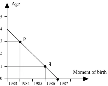
Using such a construction, all the events occurring at a precise moment in time can be located on a decreasing oblique (see figure 3). This isochronal line is called “isochrone”; its intersection with the axis of the moments of birth, determines the moment that it is represented on the diagram: in the case of figure 3, the oblique corresponds to the date 1/1/87. At this date, an individual born on the 1/1/84 was 3 years old (see dot “p”); another born on 1/1/86 was 1 year of age (see dot “q”).
Figure 3: An isochrone
Age
1983 1984 1985 1986 0
1 2 3 4 5
Moment of birth
1987
p
q
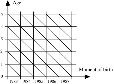
To be used easily, networks of parallel lines corresponding to particular co-ordinates complete the graph (see figure 4):
- the horizontal ones for the exact ages;
- the vertical ones for the moments of birth (corresponding to the beginning or end of the year);
Figure 4: The networks of parallels according to Lexis
Age
1983 1984 1985 1986 0
1 2 3 4 5
Moment of birth
1987
It is now easy to locate deaths on the graph:
- any death occurring between an individual's 2nd and 3rd birthday is located in a horizontal band limited by exact ages 2 and 3. A completed age thus results in a horizontal corridor (see figure 5.a, the age of 2 completed years);
- any death of an individual born in 1986 (the birth cohort or simply the cohort 1986) is located in a vertical band limited by the moments of birth 1/1/1986 and 1/1/1987 (see figure 5.a);
- any death occurring between 1/1/1986 and 1/1/1987 is located in an oblique band limited by the isochrones of 1/1/1986 and 1/1/1987; one year thus results in an oblique corridor (see figure 5.b, the year 1986);
Figure 5: The localisation of the co-ordinates
Age
1983 1984 1985 1986 0 1 2 3 4 5
Moment of birth
1987
Age
1983 1984 1985 1986 0 1 2 3 4 5 1987 5.a 5.b 2 completed years Cohort '86 Year '86 W
This construction is entirely satisfactory since it allows for the systematic location of the three demographic co-ordinates. The diagram comprises only two axes, reserved for the moment of birth, on the horizontal axis, and, for age, on the vertical one. These two ordinates are classically represented by lines perpendicular to their axis. The third co-ordinate - time or moment of death – parasites the horizontal axis (Note 5) and is figured by an oblique.
Thus the horizontal axis supports two co-ordinates: the moment of birth and the time. The moment of birth can be considered as the “host” co-ordinate, in that it welcomes on its axis another co-ordinate, time. This latter can thus be taken as a parasitical co-ordinate, for it occupies a spot on an axis which is not its own (Note 6).
Figure 6: The localisation of population figures and events
Age
1983 1984 1985 1986 0
1 2 3 4 5
Moment of birth
1987
o p m n
Cohort '84
2 completed year
Years '86 et '87
To work out his construction, Lexis passes from only one axis to a figure with two axes in order to represent three dimensions. To better understand this construction, another approach may appear more logical, namely to start from a diagram with three axes (one for each demographic co-ordinate) and to convert it into a two axes diagram. This is the subject of the next section.
2.2 From three to two axes or the emergence of three equivalent solutions
Figure 7: The three axes diagram
Age
Time M = Moment of birth
M
t(1)
t(2) 0
a
m N
D p
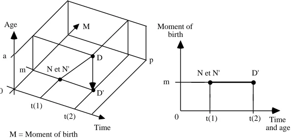
In this graphic volume, the lifeline (Note 10) of an individual born at time “t(1)” and deceased at time “t(2)” at age “a”, is limited by the following points:
- point “N”, his birth, with time co-ordinate “t(1)”, age co-ordinate “0” and moment of birth co-ordinate “m”. It should be noted that this last co-ordinate is invariant for an individual and that the segments “0m” and “0t(1)” are equal;
- point “D”, his death, with time co-ordinate “t(2)”, age co-ordinate “a” and moment of birth co-ordinate “m”. Note that “a” = “t(2)” – “t(1)”.
Due to the method of constructing the graph, all births will be on the plane “time and moment of birth”, corresponding to age “0”. More specifically, births will be aligned on the bisecting line “0 – p”. Moreover, the lifelines all incline to 45° because of the perfect correlation between time and age (Note 11). Consequently, the whole of lifelines will be placed on a plane inclined 45° and limited by the bisecting line “0 – p”. Thus, even if the graph comprises three co-ordinates, a simple plane should be enough to represent the observations.
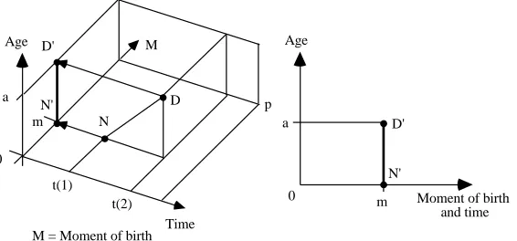
2.2.1 The “moment of birth and age” diagram
of birth co-ordinate (“m”). The point of death (“D”) moves to the vertical axis of this point “m” at the height of age “a”. Here, the “host” co-ordinate is the moment of birth and the “parasite” is the time co-ordinate. As already indicated, the graph will be completed by networks of parallels (see figure 4). On this figure, an oblique line must be interpreted in the following way: the evolution of age according to the moment of birth at a given date (see figure 3).
Figure 8: The projection on the “moment of birth and age” plane
Age
Time M = Moment of birth
M
t(1) t(2) 0
a
m N
D p
N'
D' Age
Moment of birth and time 0
a
N' D'
m
To pass from a volume to a plane, it is also possible to project on either one of the two other planes, the “time and age” plane or the “time and moment of birth” one.
2.2.2 The “time and age” diagram
Figure 9: The projection on the plane “time and age”
Age
Time M = Moment of birth
M t(1) t(2) 0 a m N D p N' D' t(1) t(2) a D' N' Age
Time and moment of birth
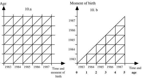
Here also the diagram will be completed by networks of parallels (see figure 10.a). In this graph, an oblique line is interpreted in the following way: the evolution of age according to time for any one moment of birth or a given individual.
Figure 10: The networks of parallels
1983 1984 1985 1986 1987 Time and 1983
1984 1985 1986 1987
Moment of birth
1983 1984 1985 1986 1987 0 1 2 3 4 5 Time and moment of birth Age 10. b 10.a age
2.2.3 The “time and moment of birth” diagram
In the case of a projection on the “time and moment of birth” plane (see figure 11), “N” and “N'” merge and “D'” is projected at the height of the moment of birth (“m”) and of the date of death (“t(2)”). Here the “host” co-ordinate is time, and the “parasite” is age. To be rigorously complete, the figure should thus comprise two scales under the horizontal axis: one for time and one for age (see figure 10.b). In the first two projections this is not the case, since the “host” and “parasite” co-ordinates correspond on the same scale!
Figure 11: The projection on the “time and moment of birth” plane
Age
Time M = Moment of birth
M
t(1) t(2) 0
a m
D p
D' N et N'
Moment of birth
Time and age 0
m
t(1) t(2) D' N et N'
Again, the diagram will be completed by networks of parallels (see figure 10.b). An oblique is interpreted as the evolution of the moment of birth according to time for a given age.
3. But who then invented the Lexis diagram?
The previous point showed that the diagram proposed by Lexis is, in fact, only one of the three solutions to get from three to two axes. In addition, the version most currently used is actually not the Lexis’ one. The form changed, the name remained. The question of paternity then can be reformulated by two more precise sub-questions:
- who was the first to suggest a satisfactory solution?
- who was the first to suggest each of the three versions of the diagram?
These two questions will be tackled after a quick summary of the controversy up to the beginning of the twentieth century which took place between several researchers.
3.1 The controversy
Since 1880 (but perhaps already before) and at least until 1903, the question of the paternity of the diagram was prone to polemics, mainly between Lexis and Zeuner. In a text of 1880, Lexis writes the following about two diagrams proposed by Becker and Verwey (Note 14):
“According to custom, the book (Note 15) is dated from 1875, even if it was published already in 1874. The foreword was written just before the publication and is dated from 1874. The impression of this book was already begun during the summer when Becker published his book. My work is completely independent of Becker’s. Soon after, Verwey published a thesis in Dutch about the same subject and the application of the same principle, but his work is independent of mine. The article of Verwey was published in English in the Journal of the Statistical Society, London, in December 1875.” Later, Zeuner will dispute the paternity assumed by Lexis in a publication of 1886 (Note 16). On page 8, one can read the following:
“Lexis uses the same figure in his book "Einleitung in die Theorie der Bevölkerungsstatistik" Strassburg 1875. This figure presents perpendicular axes. So, Lexis accepts the plan of my stereometric figure. Note by the way that Lexis does not refer to my work.” (Note 17)
Then on page 11:
In addition, Zeuner begins his text complaining about the lack of recognition of research carried out by mathematicians. To prove his point, he takes the example of Gossen’s work in political economy, ignored for more than 20 years until it was quoted by foreign economists. Implicitly Zeuner stated that some scholars (more specifically Lexis) did not understand the importance of his work on the graphical representation of population dynamics and of a clear mathematical formulation of demographic calculation.
At the beginning of the twentieth century, Lexis counterattacked (Note 18) in a footnote at the bottom of page 3. In this very long footnote, Lexis speaks about several scientists who have worked in the field of the graphical representation of population dynamics. In this footnote, Lexis tries to demonstrate that he invented his figure independently of the influence of these scientists. First Lexis says that his own book of 1875 and the publication where Becker presents in 1874 his construction are independent and that his own book was in fact already edited during 1874. Then, Lexis recognizes that his own construction and Verwey’s are the same, even if Verwey does not use death points. Lexis quotes a publication of 1875 even if Verwey had already published his work in 1874! Lexis goes on to speak a little about Brasche’s construction for which he uses the expression “rough shape”. In fact, the main part of the footnote concerns Zeuner. In Lexis’ opinion, Zeuner injuriously claims that Lexis has adopted the construction presented by Zeuner in a publication of 1869. Lexis explains that the same network of lines appears on the basic plane of the two constructions even if they follow different logics: if Lexis represents death points, Zeuner represents survivors. Lexis explains also that it is possible to obtain a stereometric figure on the basis of his construction. Finally, Lexis insists that he prefers a planimetric figure (and not a stereometric one) because its use is easier.
Other texts could undoubtedly still be quoted, but those proposed here should have made the rather long lasting controversy around the paternity of the diagram sufficiently clear.
3.2 The development of the three diagrams
3.2.1 The diagram “time and moment of birth”
Why start with this version? Quite simply because it is the version on which, to our knowledge, researchers first worked. In fact, one has to wait until 1874 for Becker to propose the complete diagram “time and moment of birth” (Note 20). Lexis recognized that Becker published his work before his own, but he considered his construction preferable to Becker’s (although the two versions are rigorously equivalent in locating events and population figures, i. e. the main purpose of this construction!). Certain German authors however, prefer Becker's version, at least for certain uses (Note 21).
To work out his diagram, Becker was largely inspired by Knapp (Note 22). The latter had already proposed a diagram in 1868 but the co-ordinate “moment of birth” was given by number of birth rather than time of birth. In fact, the space allotted to a cohort on the vertical axis varied according to the number of births. Dupâquier J. and M. indicate that Knapp in his turn had taken up an idea of Priestley going back to 1765 (Note 23).
3.2.2 The diagram “moment of birth and age"
As already pointed out, Lexis claims to have invented this diagram. Zeuner contested this claim. What can one make of this question? In a publication dating from 1869, Zeuner furnished an elegant mathematical method for calculating Knapp’s mortality table (Note 24). He based his proof on a figure whose basic plane was, in fact, a “moment of birth and age” diagram. Zeuner also used isochrone but unlike Lexis did not add the network of parallels. In addition Zeuner added to his base a vertical axis so as to represent surviving population figures. His diagram thus became a stereogram.
Except for the networks of parallels, Zeuner thus proposed a diagram “moment of birth and age” 6 years before Lexis. We do not think that the arguments developed by Lexis in 1903 (the use of the mortuary points instead of population figures of survivors, as Zeuner had, see supra) are sufficient to accept the idea that his graph and the one of Zeuner are different. Moreover, Lexis explains that it is easy to pass from Zeuner’s basic stereometric construction to his own diagram or the other way round. In fine, Zeuner as well as Lexis, manages to place the three demographic co-ordinates on the same plane, using only two axes. The advantage in terms of prior invention thus goes to Zeuner.
English article of December 1875 (Note 26). According to Lexis, his own work appeared before, namely in 1874. However, there is doubt about its effective publication, which appears to be only in 1875 (the title carries the date of 1875, but according to Lexis, the work appeared already in 1874). It is quite difficult to conclude anything definite about the anteriority of the two contributions, even if by sticking to the dates of publication the advantage goes in fact to Verwey, all the more because the argument that Lexis proposes for his publication of 1875 is undoubtedly valid also for Verwey’s publication in 1874.
3.2.3 The diagram “time and age” or Brasche, the great forgotten
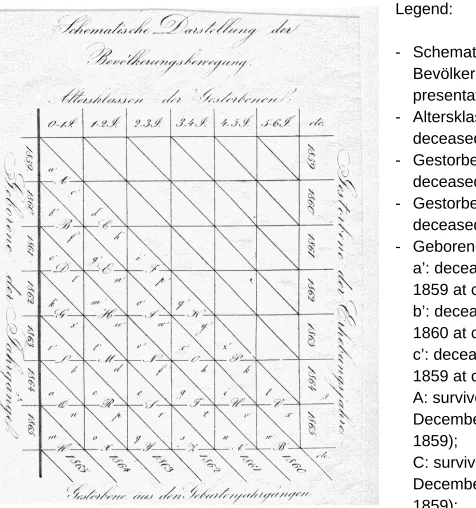
In 1870, Brasche published a work on a life table (Note 27) in which he used a diagram “time and age” with networks of parallels (see figure 12).
Figure 12: The Brache’s diagram
Legend:
- Schematische Darstellung der Bevölkerungsbewegung: schematic presentation of population dynamics; - Altersklassen des Gestorbenen: age of
deceased;
- Gestorbene der Erhebungsjahre: deceased during the year;
- Gestorbene aus den Geburtenjahrgängen: deceased of birth cohort;
- Geborene der Jahrgänge: births of years; a’: deceased during 1859 in birth cohort 1859 at completed age 0;
b’: deceased during 1860 in birth cohort 1860 at completed age 0;
Unfortunately, he is not very explicit about the construction of his graph (remark 3 page 20; for the original quotation, see appendix, section D):
“To demonstrate this proposition and the following explanations, we propose a schematic representation of population dynamics. If this figure is extended in the direction of time (…) and age until the highest age and if we consider that the relative value of the different variables has no importance, additional explanations of this figure would be useless”.
Not very loquacious about the construction of his figure, he is even less aware of a possible influence of his predecessors. By another way, Brasche remains largely unknown by his contemporaries. Zeuner, in his publication of 1885, does not refer at all to the work of Brasche, but quotes Lexis, Lewin, Becker, Perozzo, Knapp... Lexis will make an allusion to it in 1903 (and perhaps even before, but by no means in 1880) without giving it the importance it actually deserves. On the contrary, Lexis disparages the construction of Brasche as if it were just an outline, whereas it incontestably allows for a correct presentation of the lifetable indexes.
Brasche uses his graph without explaining the role of the lifelines or the mortuary points. The only thing that counts for him is the location of the population figures of deaths and survivors and to include them in his life table calculations. In 1880 Lexis agrees that this is indeed the objective of such a diagram (Note 28):
“It is not necessary that all points are figured or that their density is represented. The most important thing is always the network of lines within the death points are mentally located.”
Why then did Lexis not recognize the qualities of Brasche’s construction?
In short, Brasche is the first to propose a plane figure (without vertical axis, as proposed by Zeuner) supplemented by networks of parallels as Becker, Verwey and Lexis will do later. What merit for only one man! Around 1960, Pressat will rediscover and popularise the Brasche’s diagram. Currently, this version is actually used most often without reference to Brasche or Pressat, but with reference to Lexis!
3.2.4 The diagram race: prize giving
For the addition of the networks of parallels on a graph with two dimensions (second criterion), Brasche (1870) can be classified first, followed by Becker (1874) and finally by Verwey and Lexis, with undoubtedly a slight advantage for Verwey. Lexis thus exits the podium! With regard to the diagram “moment of birth and age”, Lexis finally appears in third position far behind Zeuner (something apparently never fully understood by Lexis himself) and just behind Verwey. At the best, Lexis can hope to share second place with Verwey.
4. Conclusions
In our opinion, to speak of the “Lexis diagram” is a misnomer. If the name should evoke the inventor, then several names would be preferable:
- Zeuner’s diagram to indicate the first author who worked out diagram on a plane (with two axes) to represent the three demographic co-ordinates;
- Brasche’s diagram to stress that he is the inventor of the plane diagram with networks of parallels; it is the version most currently used now;
- Verwey’s diagram or Verwey/Lexis diagram for the version “moment of birth and age” used by Lexis and actually rather fallen into disuse.
In spite of all this, the name “Lexis diagram” has imposed itself in a seemingly invincible way, even if, according to sources, the importance of the role played by Lexis changes. On the one hand, Seligman, for example, writes the following (Note 29):
“Special mention must be made ... of a new method of graphic treatment of mortality, first broached in his Einleitung in die Theorie des Bevölkerungsstatistik (Strasbourg 1875) and developed in later publications”. Also Petersen and Petersen consider Lexis as the father of the diagram (Note 30):
“Lexis diagram, first developed by the German statician Wilhem Lexis, has become a widely used tool in demography”.
Dupâquier J. and M. grant also priority to Lexis. After speaking about the construction of Becker, they write (Note 31):
Westergaard also mentions Verwey, but by quoting his English article and not his (earlier) Dutch thesis. Caselli and Lombardo indicate that Becker and Lexis both solved the problem of the representation of the three demographic co-ordinates on one plane (Note 33). Considering the anteriority of his publication, the advantage would go to Becker, even if the authors do not tackle this question. This idea is taken up in a Russian encyclopaedic dictionary where the contributions of Zeuner, Knapp and Becker are highlighted (Note 33); in addition, the replacement of Lexis’ version by Pressat’s is also mentioned.
The contribution of some of the authors quoted in the history of the development of the diagram is more or less regularly recognized (Knapp, Zeuner, Becker and obviously Lexis); on the other hand, others remain largely unknown (Verwey or especially Brasche). In addition, the role of Lexis in this saga differs clearly according to sources: the sole initiator according to some, a mere continuator according to others. Then why did the name “diagram of Lexis” become almost incontrovertible? In our opinion, several assumptions can be advanced:
- Lexis worked a long time on this diagram; over 30 years, he published various writings where the diagram occupies a more or less significant place. In addition, Lexis was not satisfied in merely establishing a graph; he also proposed various ways of using it, such as, for example, the representation of the numbers of varied events by different circles of various colours (Note 34). On this subject, the question one can ask is whether these innovations were useful? In our opinion, no! The modern user pays them little attention;
- Lexis seems to have been a considerable scientist in his time, undoubtedly more considered than some of his contemporaries working on this subject; his work, moreover, extended well beyond the field of population dynamics;
- Lexis also published in French, a language much used in the 19th century, thus contributing to his international reputation.
Notes
1. In this respect, we thank Mr. Pracht of Lapoutroie (France) who took charge of the major part of the translations which permitted us to do this research. We also thank Mrs. Ch. Letocart (SPED - UCL, Belgium), Mrs. Ch. Kienlen of Brunstatt (France), I. Schockaert (SPED - UCL, Belgium) and M. Singleton (SPED - UCL, Belgium). 2. In this text, we will limit ourselves to the example of deaths, even though the
method is applicable to other demographic or non-demographic phenomena. 3. Lexis W. (1880). “La représentation graphique de la mortalité au moyen des points
mortuaires”. Annales de démographie internationale, Tome IV: pp. 297 - 324. 4. Lexis hesitated with regard to the angle of rotation. At a given moment, he rather
leaned towards a slant of 60°; finally, he opted for 90° - the only case considered here.
5. One can also consider that the third co-ordinate parasites the vertical axis, but this vision of thing proves to be less convenient. One can also propose a third axis which in the present case would be an increasing oblique line inclined to 45° from the point origin, but this third axis is not essential to understand and to use this kind of diagram. Concerning this, see Barsy G. (1958). “A Csecsemöhalandosag mérése (The Measure of Infant Mortality)”. Demografia, Volume 1, N° 1: pp. 27-57. 6. In the present case, the host and parasitic co-ordinates express themselves in the
same way (the calendar), so that the coexistence of these two co-ordinates on one same axis doesn't pose any particular problem; this will not always be the case (see infra, the diagram “time and moment of birth").
9. The three axes are orthonorms. It is not an indispensable condition, but it did not appear useful to us to consider other situations, given that the three co-ordinates express themselves in the same unit, i.e. the year.
10. Here, we prefer the name “life line” to “life span”; indeed, in the diagram, exposed in the previous point, the length of the segment, representing the life of an individual, is identical to this length measured on the axis of age. It is not the case for the volume.
11. As a condition for this slant of 45°, it is necessary to recall that the axes are orthonorms. In the contrary case, the slant will be different.
12. Lexis, starting from an unique axis, succeeds in explaining without difficulty, the diagram obtained by projection on the plane “time and moment of birth”; it would be a lot more difficult for him, in following this way, to obtain the figure resulting from the projection on the plane “time and age”.
13. According to the expression of R. Pressat (letter to the author dated from March 25, 1991).
14. Lexis W. (1880). “La représentation graphique de la mortalité au moyen des points mortuaires”. Annales de démographie internationale, Tome IV: p. 298, footnote 3. (For the original quotation, see appendix, section A).
15. Lexis refers to the following publication (the first where he exposes the version of the diagram presented in the article of 1880): Lexis W. (1875). Einleitung in die Theorie der Bevölkerungsstatistik. Strassburg: Karl J. Trübner.
16. Zeuner G. (1886). “Zur mathematischen Statistik”. Beilage zur Zeitschrift des königlisch Sächsischen statistischen Bureau, XXXI Jahrgang: pp. 1-13. (For the original quotation, see appendix, section B).
of age: the numbers of births and the numbers of survivors at 0-5 years. This point will not be more developed here.
18. Lexis W. (1903). Abhandlungen zur Theorie der Bevölkerungs- und Moralstatistik. Jena: Verlag von Gustav Fischer. (For the original quotation, see appendix, section C).
19. Before concluding more definitely, it would be necessary for us to consult further texts of various authors. We think notably of Van Pesch, Lewin (not considered until now because he opted for a diagram with non perpendicular axes), Brasche (a text possibly older than the one of 1870)...
20. Becker K. (1874). Zur Berechnung von Sterbetafeln an die Bevölkerungsstatistik zu Stellende Anforderungen. Berlin: Verlag des Königlichen statistischen Bureaus. 21. See Winkler W. (1969). Demometrie. Berlin: Duncker & Humblot: pp. 90 - 91. 22. Knapp G. (1868). Die Ermittlung der Sterblichkeits. Leipzig. This publication
marks an important stage in the correct calculation of the mortality table; it enjoyed the esteem of many authors of the time of whom Zeuner, Becker and Lexis.
23. Dupâquier J., Dupâquier M. (1985). Histoire de la démographie, Collection Pour l'histoire. Paris: Librairie académique Perrin: p.122 & p. 386.
24. Zeuner G. (1869). Abhandlungen aus der Mathematischen Statistik. Leipzig: Verlag von Arthur Felix.
25. See Verweij A. (1874). De waarnemingen der bevolkingsstatistiek. Academisch Proefschrift, ter verkrijging van den graad van doctor in de wis- en natuurkunde, aan de Hoogschool te Utrecht, te verdedigen op Vrijdag den 18 December 1874, des namiddags te 3 uren. Deventer: Rustering en Vermandel and Verwey A. (1875). “Principles of vital statistics”. Journal of the Statistical Society, Volume XXXVIII: pp. 487-513. Note that the spelling of this author's name changes according to the language used: “Verweij” for the thesis in Dutch, but “Verwey” for the article in English!
28. Lexis W. (1880). “La représentation graphique de la mortalité au moyen des points mortuaires”. Annales de démographie internationale, Tome IV: p. 301. (For the original quotation, see appendix, section E).
29. Seligman E. Editor in chief. (1963). Encyclopaedia of the social Sciences. Volume nine. New York: The Macmillan Company: pp. 426-427.
30. Petersen W., Petersen R. (1986). Dictionary of Demography. Terms, Concepts, and Institutions. Volume A - M.. New York: Greenwood Press: p. 523. The commentary goes on to describe the version “time – age”, without noting that it is not the one used by Lexis.
31. Dupâquier J., Dupâquier M. (1985). Histoire de la démographie, Collection Pour l'histoire. Paris: Librairie académique Perrin: p. 386. (For the original quotation, see appendix, section F). Note that the construction of Becker also permits a solution of the passage of period analysis to cohort analysis.
32. Westergaard H. (1932). Contributions to the history of statistics. Londres: P.S. King & Son LTD: pp. 222-223.
33. Caselli G., Lombardo E. (1990). “Graphiques et analyse démographique : quelques éléments d'histoire et d'actualité”. Population, Volume 45, N° 2: pp. 402-403. 34. Great Soviet Encyclopaedia, Editor. (1994). Population Encyclopaedic. Moscow: p.
21, p. 93 & pp. 439-441.
35. See Esenwein-Rothe I. (1991). Wilhelm Lexis. Demograph und Nationalökonom (1837 - 1914). Erlangen: Jung & Sohn.
36. Lexis refers to the following publication (the first where he exposes the version of the diagram presented in the article of 1880): Lexis W. (1875). Einleitung in die Theorie der Bevölkerungsstatistik. Strassburg: Karl J. Trübner.
References
Barsy G. (1958). “A Csecsemöhalandosag mérése (The Measure of Infant Mortality)”.
Demografia, Volume 1, N° 1: pp. 27-57.
Brasche O. (1870). Beitrag zur Methode der Sterblichkeitsberechnung und zur Mortalitätsstatistik Russland’s. Würzburg: A. Struber’s Buchhandlung.
Caselli G., Lombardo E. (1990). “Graphiques et analyse démographique : quelques éléments d'histoire et d'actualité”. Population, Volume 45, N° 2: pp. 399-414. Dupâquier J., Dupâquier M. (1985). Histoire de la démographie, Collection Pour
l'histoire. Paris: Librairie académique Perrin.
EsenweinRothe I. (1991). Wilhelm Lexis. Demograph und Nationalökonom (1837 -1914). Erlangen: Jung & Sohn.
Great Soviet Encyclopaedia, Editor. (1994). Population Encyclopaedic. Moscow. Knapp G. (1868). Die Ermittlung der Sterblichkeits. Leipzig.
Knapp G. (1874). Theorie des Bevölkerungs-wechsels. Brunswick: Druck und Verlag von Friedrich Vieweg und Sohn.
Lexis W. (1875). Einleitung in die Theorie der Bevölkerungsstatistik. Strassburg: Karl J. Trübner.
Lexis W. (1880). “La représentation graphique de la mortalité au moyen des points mortuaires”. Annales de démographie internationale, Tome IV: pp. 297 - 324. Lexis W. (1903). Abhandlungen zur Theorie der Bevölkerungs- und Moralstatistik.
Jena: Verlag von Gustav Fischer.
Petersen W., Petersen R. (1986). Dictionary of Demography. Terms, Concepts, and Institutions. Volume A - M.. New York: Greenwood Press.
Pressat R. (1961). L'analyse démographique. Paris: Presses Universitaires de France. Seligman E. Editor in chief. (1963). Encyclopaedia of the social Sciences. Volume nine.
New York: The Macmillan Company.
Vandeschrick C. (1992). “Le diagramme de Lexis revisité”. Population, Volume 47, N° 5: pp. 1241-1262.
Verweij A. (1874). De waarnemingen der bevolkingsstatistiek. Academisch Proefschrift, ter verkrijging van den graad van doctor in de wis- en natuurkunde, aan de Hoogschool te Utrecht, te verdedigen op Vrijdag den 18 December 1874, des namiddags te 3 uren. Deventer: Rustering en Vermandel.
Verwey A. (1875). “Principles of vital statistics”. Journal of the Statistical Society, Volume XXXVIII: pp. 487-513.
Winkler W. (1969). Demometrie. Berlin: Duncker & Humblot.
Westergaard H. (1932). Contributions to the history of statistics. Londres: P.S. King & Son LTD.
Zeuner G. (1869). Abhandlungen aus der Mathematischen Statistik. Leipzig: Verlag von Arthur Felix.
Appendix A. Original quotations
Section A
Lexis W. (1880). “La représentation graphique de la mortalité au moyen des points mortuaires”. Annales de démographie internationale, Tome IV: p. 298, footnote 3.
“Le titre (Note 36) porte selon l'usage de librairie la date de 1875, quoique l'ouvrage eût déjà paru en 1874. La préface écrite immédiatement avant la publication est datée de 1874, et l'impression avait déjà commencé pendant l'été en même temps que paraissait le travail de Becker, dont le mien est entièrement indépendant. Une thèse doctorale de Verwey, en langue hollandaise, traitant du même sujet et de l'application du même principe parut peu de temps après, mais n'avait pas de rapport avec mon travail. L'article de Verwey a été publié en anglais dans le Journal of the Statistical Society, Londres, décembre 1875”.
Section B
Zeuner G. (1886). “Zur mathematischen Statistik”. Beilage zur Zeitschrift des königlisch Sächsischen statistischen Bureau, XXXI Jahrgang: pp. 1-13.
Page 8:
“Lexis benutzt dieselbe graphische Darstellung in seinem Buche : “Einleitung in die Theorie der Bevölkerungsstatistik” Strassburg 1875, mit rechtwinkligen Axen, hat daher den Grundriss meiner stereometrischen Darstellung einfach acceptirt, nebenbei bemerkt ohne jeden Hinweis auf dieselbe”.
Page 11:
Section C
Lexis W. (1903). Abhandlungen zur Theorie der Bevölkerungs- und Moralstatistik. Jena: Verlag von Gustav Fischer: footnote page 3.
“Strassburg 1875. Die Schrift wurde schon 1874 gedruckt und ist von der eben erwähnten Abhandlung Beckers ganz unabhängig entstanden. Fast ganz dieselbe Konstruktion, jedoch ohne Anwendung der Sterbepunkte, in einer ursprünglich holländisch erschienenen Doktordissertation von Verwey, die in englischer Uebersetzung im Journal of the Statistical Society, Dezember 1875, veröffentlicht ist. Ansatz zu einer ähnlichen Konstruktion auch bei Brasche, Beitrag zur Methode der Sterblichkeitsberechnung, Würzburg 1870. Zeuner hat (Abhandlungen zur mathematischen Statistik, Leipzig 1869) eine stereometrische Konstruktion angewandt, indem er die Knapp'schen Doppelintegrale räumlich veranschaulichte. Es ist durchaus unberechtigt, wenn Zeuner (dessen Schrift ich übrigens in meiner Einleitung in die Theorie der Bevölkerungsstatistik, S. 33 und auch in dem französischen Text der vorliegenden Abhandlung angeführt habe) in einer späteren Arbeit (Beilage zur Zeitschrift des sächs. statistischen Bureaus, XXXI, Dresden 1886) behauptet, meine Konstruktion sei dem Grundriss seiner stereometrischen Darstellung entnommen. Ich bin von einer ganz anderen Vorstellung ausgegangen als Zeuner, und wenn dabei dieselbe Form eines Netzwertes entstand, wie in dem Zeuner'schen Grundriss, so ist doch der Inhalt desselben gänzlich verschieden gedacht. Bei meiner Darstellung handelt es sich um die mit verschiedener Dichtigkeit in der Ebene verbreiteten Sterbepunkte und wenn man von dieser planimetrischen zu einer stereometrischen Vorstellung übergehen wollte, so hätte man nur Senkrechte in der Grundebene proportional der Punktendichtigkeit an ihren Fusspunkten zu errichten und deren oberen Endpunkt durch eine Fläche zu verbinden.
ff. gezeigt. Es war aber gerade meine Absicht, statt der stereometrischen Konstruktion eine möglichst einfache planimetrische zu geben, die ohne umständliche Zeichnungen die so höchst elementaren Beziehungen, um die es sich hier handelt, sofort erkennen lässt. Dass dabei die Einzelfälle durch diskrete Punkte dargestellt oder vielmehr dargestellt gedacht werden, kann nur als ein Vorteil der Methode angesehen werden, da es der Wirklichkeit entspricht und überdies sowohl die Schnittpunkte der isochronischen Linien wie auch die Punkteninhalte der Elementargesamtheiten wirklich, nämlich durch Volkszählungen und durch kombinierte Erhebung des Geburtsjahrs und des Altersjahrs der Verstorbenen, gezählt werden können. Zu Demonstrationen aber können körperliche Modelle, wie Bodio solche hat herstellen lassen, immerhin zweckmässig sein”.
Section D
Brasche O. (1870). Beitrag zur Methode der Sterblichkeitsberechnung und zur Mortalitätsstatistik Russland’s. Würzburg: A. Struber’s Buchhandlung: remark 3, page 20.
“Zur nähern Veranschaulichung dieses Satzes sowohl als der nachfolgenden Erörterungen wurde auf der lith. Tafel die schematische Darstellung der Bevölkerungsbewegung entworfen. Denkt man sich das Schema in der Richtung der Zeit (nach oben und unten) beliebig erweitert und die Anzahl des Columnen der Altersclassen des Gestorbenen fortgesetzt bis zu den höchsten vorkommenden Altersclassen, berücksichtigt man ferner, dass die relative Grösse der einzelnen Felder bedeutungslos ist so dürfte wohl das im Folgenden Enthaltene jede weitere Erläuterung des Schema‘s überflüssig machen”.
Section E
Section F
Dupâquier J., Dupâquier M. (1985). Histoire de la démographie, Collection Pour l'histoire. Paris: Librairie académique Perrin: p. 386.