Mesh Smoothing with Global Optimization under Constraints

Mesh Smoothing with Global Optimization under Constraints

Kulovec, S. ‒ Kos, L. ‒ Duhovnik, J.

Simon Kulovec* _{‒ Leon Kos ‒ Jožef Duhovnik}

University of Ljubljana, Faculty of Mechanical Engineering, Slovenia

Mesh (pre)processing remains an important issue for obtaining useful meshes used in mechanical engineering, especially for finite element calculations. An efficient and robust combination of constrained mesh smoothing together with global optimization based algorithm is presented. In contrast to other “popular” mesh smoothing algorithms that use only local diffusion approaches to smoothing we propose Lagrange-Newton Sequential Quadratic Optimization (LNO) with constraints that can satisfy local and global cost functions, respecting posed constraints. Local cost function is modeled with local average edge length, while global cost function includes barycenter and global average edge length.

Experiments with triangular, quadrilateral, and mixed meshes show flexibility of the proposed method to achieve near ideal elements for given input meshes. Convergence is presented for several 2D and 3D meshes. Various additional goals can be mixed over the area of interest with applied weights. In contrast to other methods, unconstrained meshes still preserve their global shape while improving local quality.

©2011 Journal of Mechanical Engineering. All rights reserved.

Keywords: smoothing, sequential quadratic optimization, SQO, mesh structure, geometry, vertex, cost function

0 INTRODUCTION

Mesh optimization methods are used in mechanical engineering applications areas such as solid and fluid dynamics, heat transfer, material science etc. The numerical investigation of these physical problems may require fine grained meshes over a single area of a physical model to resolve large solution variation. Even some commercial software still has problems with fine mesh generation, thus assuring effective and robust adaptive grid methods for such problems is still necessary. Currently, the majority of virtual reality applications use triangular meshes as their fundamental modeling and rendering is primitive. Such meshes can be the result of the modeling software, or may be an output of a scanning device. Their properties are often not considered as meshes with high quality. They have a non-ideal mesh elements and bad vertex connectivity. With mesh optimization one can systematically achieve improved mesh quality that will provide a reliable analysis. The purpose of this paper is to show effective mesh optimization technique that ensures better mesh structure and is applicable to general meshes. Improvements in mesh are obtained by just repositioning of vertices without changing connectivity. I.e., the position of the

mesh vertices is modified, but the mesh topology remains unchanged. While internal mesh vertices are freely movable, external vertices must often remain fixed on boundaries. Moving (or shifting) vertices can have a drastic effect on the quality of a mesh and it is more efficient than refinement and collapsing vertices especially when the translation amplitudes are small. Such mesh relaxation can be regarded as mesh smoothing as it results in a visually pleasing mesh that follows some local or global rules.

non-manifold ones, (e) cost function can be weighted and extended with additional functionals, (f) pre-calculates average edge lengths at every iteration step. This ensures very fast convergence and flexible vertex movement.

In practical implementation of general purpose LNO theory the input mesh structure is processed using .OBJ or .STL file format. The source code is written in the C++ programming language. For the mesh handling, we used an open-source library (Open Mesh).

The motivation of the work presented is to propose and analyze reasonable cost functions and to compare how they perform in “benign” situations and to identify the most promising ones for application on difficult problems. This paper considers only meshes in which the vertices are moved with a fixed connectivity with applied movement constraints on the boundary vertices.

The paper is organized as follows. Section 1 describes the basics of a constrained optimization, Sequential Quadratic Optimization, Lagrange Newton Optimization, and connections between these two methods for general meshes. Section 2 discusses cost functions followed by differences between global and local constraint optimizations. In Section 3 several complex meshing examples are presented to demonstrate the effectiveness and the effect of the proposed mesh optimization method. After discussion of the results, conclusions are given in Section 4.

1 BACKGROUND

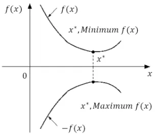
In a general optimization, the aim is to obtain the best result under given circumstances. The ultimate goal of an engineer‘s decisions is to minimize the effort required or to maximize the desired benefit. An optimization can be defined as a process of finding the conditions that give the maximum or the minimum value of a function [10]. From Fig. 1 it can be seen that if the point x*

corresponds to the minimum value of the function

f(x), the same point also corresponds to the maximum value of the negative of the function.

Constrained optimization techniques can be classified into two main categories: the direct and the indirect methods. The constraints in the direct methods are handled in an explicit manner, whereas in most of the indirect methods,

the constraint problem is solved in a sequence of unconstrained minimization problems. Our mesh optimization problem is an indirect optimization technique using the method of sequential quadratic programming.

Fig. 1. The minimum of f(x) and the maximum of - f(x) are the same values of x*

1.1 Sequential Quadratic Optimization

The SQO is considered as one of the best iterative optimization techniques. The method can be divided into two theoretical bases: (i) a set of nonlinear equations is solved by using the Newton’s method, and (ii) a Lagrangian function formed with Kuhn-Tucker conditions. Find the solution of:

x f x

H x c x

x H n

* _{arg min ( ),}

( ) .

=

=

{

}

∈

 0 (1)

Here ci is the ith component of a constrained

function c_:n _r_{. Now the Lagrange’s}

func-tion can be written:

L(x,λ) = f(x)‒λT_{·c(x), (2)}

with the gradient

L x L x

L x

f x J

c x

x cT

' '

'

'

, ( , )

( , ) ( ) ,

λ λ

λ

λ

λ

( )

  



  =

( )

   

and the Jacobian matrix of the constraint c is:

J c

x x c ij i

j

( )

At the stationary point xs is L'(xs, λs) = 0,

Thus, a non-linear system of equations is obtained:

Find (x*_{, λ}* _{) to satisfied L}’_{(xs, λs) = 0.}

To solve this problem, the Newton-Raphson’s method can be used. In each iteration step, the next iterate solution is found as (x+h, λ+η). Each step is determined by

L''_{(x,λ) [h η]}T_{= ‒L}′_{(x,λ), with:}

L L L

L L W J J xx x x cT c '' '' '' '' '' , =       = − −         λ

λ λλ 0

where W L x= ''_xx

( )

L x_xx f x _ir c x

i i '' _{( , )λ =} ''_{( )− λ} ''_{( ).}

= Σ ₀

When one Newton-Raphson step is solved by x=x+h, λ=λ+η, ,and elimination of η:

W J

J

h f x

c x cT c − −               = − −_      0 λ '_{( )}

( ) . (3)

Eq. (3) gives the solution h and the corresponding Lagrange multiplier vector λ to the following problem:

Find h argmin= e∈

{

}

In the next step, a constant

q h

_{( )}

_{( )}

con-straints lin =

{

( )

}

1.2 Lagrange Newton Optimization

LNO is a kind of Sequential Quadratic Optimization [1]. The name Lagrange-Newton comes from the two steps: in the first one, a Lagrangian function is optimized followed by the second, the Newton step when a new solution achieved. The first efficient implementations were developed by Han (1976) and Powell (1977) [1]. Currently, it is considered as the most efficient method.

The LNO method includes a soft line search with a special type of the penalty function. The description with an update method for the Hessian matrix can be concluded. This makes the method a Quasi-Newton [1] with a good final convergence without having to implement second derivates.

First, a quadratic model q of a cost func-tion in neighborhood of x is considered,

f x q

f x Tf x TW x

+

(

)

( )

( )

( )

( )

δ δ

δ ' _{1 2/} δ δ_,

then, a feasible region is defined,

H d i r

d i i r m

n i i = ∈ = = ≥ = +         δ δ δ ( ) , , , ( ) , , , . ... ... 0 1 1

Corresponding to a linear model, the constraints: c x

(

)

( )

( )

( )

First the step parameter α and matrix W(x) need to be calculated.

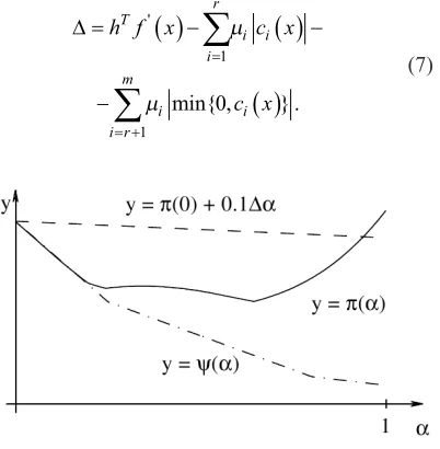
Next, the step length alpha must be calculated. If h turns out to be too large, the quadratic model may be a poor approximation of the true variation of the cost function. Therefore, a soft line search is made (a so-called exact penalty function) described in Fradsen [1]. For μi ≥ |λi| is:

π µ µ

µ

y f y c x

c y i r i i i r m i i , ( )

min , ( ) .

(

)

( )

{

}

∑

∑

The choice of the penalty factor is divided into two parts: (i) the first iteration step μ ≥ |λ|, and

(ii) the later iteration steps:

µ_i=max

{

(

)

}

The linear approximation for ci(y)=ci(x+αh)

is: π α ψ α α µ α µ

( )

( )

( )

( )

( )

∑

∑

f x h f x

c x h c x

T

i r

i i T i

i r m i ' '_{( )} 1 1 m

min{ ,_{0c x h c x}'( )} .

i

( )

(6)

∆ =

( )

( )

( )

∑

∑

h f x c x

c x T i r i i i r m i i '

min{ , } .

1 1 0 µ µ (7)

Fig. 2. Approximation ψ(α) of the line search function π(α)

To approximate π(t) on the interval

[0, α] the second order polynomial

P(t) = π(0) + Δt + (π(α) ‒ π(0) ‒ Δα) t2 _{⁄ α}2 _{is used.}

If the coefficient t2 _{> 0, then polynomial has a}

minimizer: β π α π α α =

( )

( )

2( 0 ∆ ). (8)

The iteration procedure calculation of

α = min{0.9α, max{β, 0.1α}} is repeated until π(α) ≥ π(0) + 0.1Δα.

For the next iteration step, it is required to update W(x), which for the first iteration equals I.

In the next iteration steps:

W x

( )

The change in the gradient of Lagrange’s function is:

y L x L x

f x f x J x J x

x new x

new c new c T

=

(

)

( )

(

)

( )

(

(

)

( )

)

λ (10)

where xnew = x + αh.

In each iteration, the curvature condition,

yT _{(xnew‒x) > 0 must be checked If the condition}

does not satisfy Wnew = W, then for u = Wh:

W W

h yyy h uuu

new= +_α1T T− T1 T. (11)

The whole procedure of the Lagrange Newton method is repeated until the stop criterion is satisfied. For x= xprev + αh. the stop criterion is:

η α

λ λ

x q h f x

c x c x

i i i

i

i

, ( )

( ) min , ( ) ,

( )

( )

+ +

{

}

∈ ∈

∑

∑

L M

0 (12)

where  is a set of active inequality and equality constraints, and  is a set of inactive inequality constraints.

2 COST FUNCTIONS DEFINITION

First, a definition of two optimization cost functions with the constraints: (i) local and (ii) global is given. The cost functions will be formed from mesh vertices. In our case, the functions will ensure similarity of mesh elements (equal triangles, quads, etc. in one 2D mesh structure) on the (i) local and (ii) global level. The most important constraint is that the vertices are moved with a fixed connectivity. That means the vertices must be connected with the same edges even after optimization.

2.1 Local Cost Function

In the first step the equation of the local average length is defined:

l

v v

p i n

av i

i j i j j p ( , ) ( , ) ( , ) , . = + = = − =

∑

0 _{for 1to} (13)

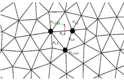
Let us begin with the vertex of the mesh structure vi,j. Operator || || is the Euclidian norm

operator. Indices i and j define vertex position in the mesh structure. Index i represents the number in the mesh structure vertices (i = 1 to n) and index j represents any mesh element of the mesh structure ( j = 1 to m). xi,k

(triangle, quad, etc.) are the edge lengths. The mesh elements in Fig. 3 are represented by indices

i and k. Index k represents the kth _{edge of the local}

mesh element (k = 1 to p). There are three constant values for the input mesh structure: (i) number of all vertices n), (ii) number of all mesh elements

m), and (iii) number of edges in one mesh element

Fig. 3. Triangular mesh elements presentation

In the second step the local cost function is defined:

f_local v v l

i m

j p

i j i j av i

=

(

)

= −

= −

+

∑∑

0 1

0 1

1

2

, , , . (14)

Eq. (13) presents the average local length of an input mesh element (triangle, quad, etc.). For variables introduced in Eq. (13) see Fig. 3.

2.2 Global Cost Function

In this cost function pre-calculated average edge lengths are used. The edge lengths are constant during iterations and can thus be considered as global. The lobal cost function is defined as:

f_global v v l

i m

j p

i j i j av gl

=

(

)

= −

= −

+

∑∑

0 1

0 1

1

2

, , , , (15)

with the global average length (see Fig. 4):

l v v

m p

av gl i m

j p

i i ,

, ,

.

= −

+ =

− = −

+

∑ ∑

0 1

1 0 0

(16)

The set of nonlinear equations is solved using the Lagrange-Newton optimization method. The LNO method searches the design vector solution X=

{

}

f(x).

The design vector x1 for i = 1 to n is a set of optimized vertex coordinates.

Fig. 4. Quadrilateral mesh elements presentation

2.3 Smoothing Methods

The most common smoothing method is Laplacian [2], where each vertex is moved to the centroid of its neighbors. Laplacian smoothing defines the number of adjacent vertices to vertex

i with ℵ =_i

{

}

The Lennard-Jones potential [3] from chemistry describes attraction/repulsion behavior. Its smoothing function is f(d) = d‒13_{‒ d}‒4_{. This}

model suffers from numerical instabilities.

The Pliant method with re-triangulation [4] uses f(d) = (1‒d4_)·exp(‒d4_{). The goal of the}

method is to create meshes with normalized edge length of 1. Reasoning behind this smoothing function is that if two vertices are too close to each other (d < 1), they repel, and if they are too distant (d > 1), they attract each other.

In our mesh smoothing optimization local (LCF) and global (GCF) cost function (Sec. 2.1 and 2.2) optimization is proposed. The main advantage of our optimization method is global mesh structure optimization. That means that all the vertices in mesh structure are repositioned in one iterations step. Other methods use just one vertex (diffusion) repositioning per iteration step.

With the local cost function vertices of mesh structure are moved to ensure equal edge lengths of faces. In contrast to other smoothing methods our LCF method calculates average edge lengths in every iteration step for all faces. This ensures flexible vertices in the mesh structure.

are calculated before smoothing begins. Our optimization algorithm can ensure approximately equal external form as the initial mesh structure even after optimization without boundary constraints.

3 RESULTS

At the beginning the results of this optimization method with two different cost functions applied to many different data sets, ranging from small sets sampled from simple mesh structures to complex models with many vertices, are showed. For the small samples, the final vertices positions are known.

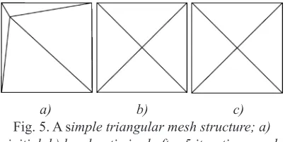
a) b) c)

Fig. 5. A simple triangular mesh structure; a) initial, b) local optimized after 5 iterations, and

c) global optimized after 4 iterations meshes

a) b)

Fig. 6. Convergence of a) local after 5 and b) global cost functions after 4 iterations

We began with a simple triangular mesh with fixed boundary mesh elements. Then, the center vertex was moved into some extreme position (see Fig. 5).

In the next step the LNO algorithm was applied. The expected result after LNO is to have a vertex in middle position of boundary area. In Fig. 3 results for two different cost functions and LNO results for local (see Fig. 5b) and global (see Fig. 5c) oriented cost functions are presented. In this case the results are equal. Using global iteration is favorable due to faster convergence.

The second “trivial” example for testing the LNO algorithm is quadrilateral mesh structure shown in Fig. 7.

a) b) c)

Fig. 7. Simple quadrilateral mesh structure; a) initial, b) local optimized after 4 iterations, and c)

global optimized after 3 iterations meshes

a) b)

Fig. 8. Convergence of a) local after 4 and b) global cost functions after 3 iterations

The result of the LNO method are four equal square elements in the input mesh structure for the local and global cost functions. A similar result for the vertex positions after application of the LNO algorithm is expected. The difference between the local (Fig. 6b) and the global (Fig. 6c) optimization result is usually within few iteration steps.

Fig. 9. Initialquadrilateral mesh structure with equidistant boundary mesh vertices

vertices and 24 external (boundary) vertices that are fixed and equidistant. The LNO method for two different cost functions and the same con-straints (local and global cost functions) is done first. The results for the local cost function are presented in Fig. 10a. For the global cost function, see Fig. 10b. After optimization there are equal mesh elements (squares) in both optimization re-sults. Despite different cost functions, the same vertices positions are obtained after 30 iteration steps for the local and global cost function.

a) b)

Fig. 10. a) Local; and b) global optimized mesh structure after 30 iteration steps

For all simple examples tested the optimal vertices positions are known. In the first case, four equilateral triangles and for the second and the third example equilateral squares were expected. Initial examples show the accuracy of the LNO algorithm that is implemented in C++ language.

a) b)

Fig. 11. Convergence of a) local; and b) global cost functions after 30 iterations

3.1 Triangle Meshes

Let us begin with a more complex triangular mesh structure [5] optimization. In Fig. 12 a triangular mesh with several vertices is shown. The triangular mesh structure with two different cost functions and two different types

of constraints was optimized. For LNO local and global cost functions were used. Different constraints were also used: (i) variable and (ii)

fixed boundary mesh vertices.

Fig. 12. Initial triangular mesh structure

For the mesh optimization, shown in Fig. 12, different combinations of constraints and cost functions were attempted. In the first combination the local cost function and a constraint with variable boundary mesh vertices were used. The first combination result is presented in Fig. 13a after 50 LNO iterations. The resulting mesh is not very useful because the boundary vertices are moved and the triangle mesh elements are not equal.

a) b)

Fig. 13. a) Local, and b) global optimizations after 50 iteration steps with variable boundary

mesh vertices

a) b)

Fig. 14. Convergence of a) local, and b) global cost functions after 50 iterations

a) b)

Fig. 15. a) Local, and b) global optimizations after 30 iteration steps with fixed boundary mesh

vertices

Large boundary vertices deviations in the previous optimizations are prevented with fixed boundary vertices in the following examples. Let us make combinations of the local and global cost functions inside fixed boundary vertices. With fixed boundaries, it is ensured that the initial boundary vertices remain fixed during optimization. In Fig. 15a the optimized mesh

structure with the local cost function is shown. The mesh structure was reached after 30 iteration steps. The optimized mesh structure is composed of almost the same triangles but still with some exceptions which cannot be fixed with this optimization algorithm. In Fig. 15b the optimized mesh structure with the global cost function is presented. The global cost function ensures that the initial average edge length during optimization is preserved. The mesh structure converged after 50 iterations.

Both mesh results are similar (see Fig. 15). The local cost function is faster because the variable edge length in a local optimization is more flexible.

a) b)

Fig. 16. Convergence of a) local, and b) global cost functions after 30 iterations

The final conclusion for triangle mesh structures is that the constraints in such optimi-zations must be applied to prevent changes of the initial boundaries. Comparing the initial (see Fig. 12) and the optimized mesh structures (see Fig. 15a), it can be concluded that the mesh after optimization has a better distribution of the mesh triangle elements and almost equal mesh elements over the whole mesh structure.

3.2 Quad Meshes

In this section the LNO method is applied on a more complex quadrilateral mesh structure. Let us optimize the initial quadrilateral mesh structure shown in Fig. 12. The initial mesh structure was optimized with the local and global cost functions and two different constraints.

control over the mesh structure result. This means it was not known whether the initial mesh would roughly keep the initial boundary shape. As there were no constraints, the convergence of the LNO algorithm could not be expected.

Fig. 17. Initial quadrilateral mesh structure

a) b)

Fig. 18. a) Local, and b) global optimizations after 70 iteration steps with variable boundary

mesh vertices

a) b)

Fig. 19. Convergence of a) local, and b) global cost functions after 70 iterations

The result of the unconstrained mesh optimization after 70 iteration steps is shown in Fig. 18. In both meshes the boundary vertices were moved. The edge lengths are equal all over the mesh structure in both cases. However, in the global optimization case the mesh elements are almost square.

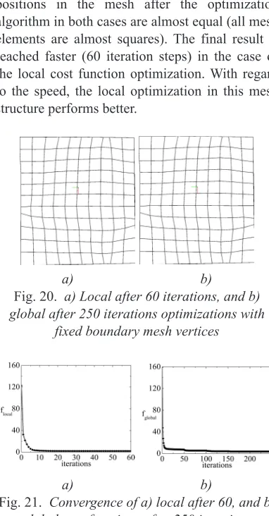
Let us look at the mesh optimization results with constraints as shown in Fig. 20. The constraints were fixed boundary vertices. With

this constraint, the possibility that the optimization algorithm changed the initial boundary position is disabled. It can be concluded that the vertices positions in the mesh after the optimization algorithm in both cases are almost equal (all mesh elements are almost squares). The final result is reached faster (60 iteration steps) in the case of the local cost function optimization. With regard to the speed, the local optimization in this mesh structure performs better.

a) b)

Fig. 20. a) Local after 60 iterations, and b) global after 250 iterations optimizations with

fixed boundary mesh vertices

a) b)

Fig. 21. Convergence of a) local after 60, and b) global cost functions after 250 iterations

First of all it can said that the LNO algorithm is convergent for constrained and unconstrained quadrilateral meshes. Like in the case of the triangle mesh optimization, constrained optimization gives better results (more squares in the mesh structure) compared to the unconstrained optimization. Finally, it can be concluded that a quadrilateral mesh optimization with local and global cost functions can be used in practice (FEM, CFD, etc.).

3.3 Numerical Examples

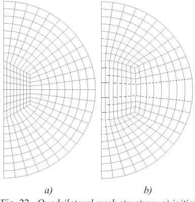
of optimization algorithm is shown in Figs. 22 to 26. The initial grid (see Fig. 22) consists of two blocks generated subgrids corresponding to a trapezoidal subdomain and its continuation to the annular region. Boundary vertices on the exterior boundary are fixed and other vertices are allowed to “slide” like in the Branets-Carey [6] numerical example.

a) b)

Fig. 22. Quadrilateral mesh structure; a) initial and, b) combination of barycenter and local cost

functions

Fig. 23. Convergence of mesh structure for combination of barycenter and local cost

functions after 150 iterations

Fig. 22 presents the initial quadrilateral mesh, which is the same as in Branets-Carey [6]. For optimization external vertices in mesh structure are used. The cost function is a combination of local and barycenter cost functions with weights. Barycenter is cost function which tends to equal diagonal of quadrilateral element.

The weight for the local cost function is wl = 0.3

and the weight for barycenter is wb = 0.3. In Fig.

22 optimized initial quadrilateral mesh structure with a combination of local and barycenter cost functions after 150 iterations is also demonstrated.

Minimization of quadrilateral mesh (see Fig. 22) cost function as the function of the number of iterations is presented in Fig. 23.

a) b)

Fig. 24. Combination of a) barycenter with global, and b) local with barycenter cost functions of quadrilateral mesh structure

a) b)

Fig. 25. Convergence of mesh structure for: a) barycenter with global cost functions after 350,

and b) local with barycenter cost functions after 200 iterations

The above examples (Fig. 24) demonstrate two optimized mesh structures. The left example is the optimized mesh structure with a combination of the global with weight

wg = 0.3 and barycenter with weight wb = 0.7 cost

In Fig. 25 convergence of global and local cost functions in combination with barycenter is shown. The convergence in graph (see Fig. 25a) is similar like the one in the graph depicted in Fig. 23. The main differences are cost function values. It can be noticed that the curve in Fig. 25b shows faster convergence in comparison with the other two graphs.

a) b)

Fig. 26. Combination of a) global with barycenter and; b) local with barycenter and

global cost functions of quadrilateral mesh structure

The last 2D mesh examples demonstrate mesh optimization combination of the global cost function with weight wg = 0.7 and barycenter with

weight wb = 0.3 after 200 iterations. The final

example presents the optimized mesh structure in combination of: global (wg = 0.3), local

(wl = 0.3) and barycenter (wb = 0.3) cost functions

after 70 iterations.

Fig. 27 presents convergences of cost functions for quadrilateral mesh structure optimization.

The goal is also to improve the quality of the 3D mixed mesh structure (see Fig. 28) optimized with global and local cost functions in combination with the barycenter cost function. There is the initial 3D mesh structure with main quad elements and some triangle elements on boundaries.

a) b)

Fig. 27. Convergence of a) global with barycenter cost functions after 200 and, b) local with barycenter and global cost functions after 70

iterations

Fig. 28. Initial mixed 3D mesh example

Fig. 29. Optimization of mixed mesh structure with local and barycenter cost functions

Fig. 29 demonstrates the smooth behavior of mixed 3D mesh using local (wl = 0.6) and barycenter (wb = 0.4) cost functions.

After the applied optimization quadrilateral mesh elements with equal diagonals and equal length of triangle element sides are obtained.

The mesh structure shown in Fig. 30 is optimized with global (wg = 0.6) and local

(wb = 0.4) cost functions. The main difference

of previous mesh structure is in values of cost functions during iterations (see Fig. 31).

Fig. 31 presents the convergence of local and global cost functions in combination with barycenter after 30 iterations.

Fig. 31. Convergence of mixed mesh structure for: a) local with barycenter, and b) global with

barycenter cost functions after 30 iterations

3.4 Discussion

The examples show optimizations of triangular, quadrilateral and mixed mesh structures. For every mesh type our optimization algorithm shows improved mesh structure. This is important for triangular mesh structures which are currently used for majority applications.

For the optimization local and global cost functions are proposed. For the optimization of unconstrained mesh structure it is better to use global cost function, while the local cost function performs better on constrained mesh structures. The global based algorithm ensures mesh smoothing with respect to all mesh vertices in one iteration step.

For a comparison of optimization quality of quadrilateral mesh structure Branets-Carey [6] mesh example was taken. The last example is 3D mixed mesh structure. There is the 3D mesh example with the main quadrilateral mesh elements and triangle mesh elements in external edges. In both cases optimizations repaired the mesh structure and have had cost functions convergence. Within optimization quads with

equal diagonals and triangles with almost equal sides can be mixed.

Other popular mesh smoothing algorithms (Laplacian [2], Lennard-Jones [3], and Pliant [4]) are only local diffusion approaches. At the same time the optimization algorithm in question possesses fast convergence. In other algorithms mixed mesh optimization examples were not observed.

4 CONCLUSIONS

This paper has focused on the applicative use of the constraints in mesh optimization and defined cost functions to ensure mesh quality. For testing the Lagrange Newton Optimization algorithm, several examples were used. For these examples, the optimal vertices positions were known. The cost functions were stated in terms of vertices based geometric entities. The cost functions were implemented in a post-processing procedure and shown to be effective in achieving good element quality in several problems. The same cost functions that were effective on quadrilateral meshes were also effective on triangular ones. The speed and efficiency issues were not considered although it has been observed in practice that no significant time penalty applies to optimization with one cost function as compared to another.

The results for triangular meshes are achieved in a few iteration steps. In the quadrilateral mesh optimization, the priority of LNO is to ensure more equal mesh elements (almost all elements in the mesh structure were squares).

5 REFERENCES

[1] Madsen. K., Nielsen. H.B., Tingleff, O. (2004). Optimization with constraints, 2nd _ed.

IMM, Technical University of Denmark, Kgs. Lyngby.

[2] Field, D.A. (1988). Laplacian smoothing and Delaunay triangulations. Comm. Applied Numer. Meth., vol. 4, p. 709-712.

[3] Allen, M.P., Tildesley, D.J. (1987). Computer simulation of Liquids. Claredon Press, Oxford.

[4] Pascal, J.F., Houman, B. (1998). Geometric surface mesh optimization. Comput Visual Sci, vol. 1, p. 113-121.

[5] Vukašinović, N., Korošec, M., Duhovnik, J.

(2010). The influence of surface topology on the accuracy of laser triangulation scanning results. Strojniški vestnik - Journal of

Mechanical Egineering, vol. 56, no. 1, p. 23-30.

[6] Branets, L., Carey, G.F. (2005). A local cell quality metric and variational grid smoothing algorithm. Engineering with Computers, vol. 21, p. 19-28.

[7] Madsen, K., Nielsen, H.B., Tingleff, O. (2004). Methods for non-linear least squares problems, 2nd edition. IMM, Technical University of Denmark, Kgs. Lyngby.

[8] Arora, J.S. (2004). Introduction to optimum design. Elsevier, Academic Press, San Diego. [9] Mulmuley, K. (1994). Computational

geometry: An introduction through randomized algorithms. Prentice Hall, Inc. [10] Knupp, P.M. (2000). Achieving finite mesh

quality via optimization of the Jacobian

matrix and associated quantities. Part I-a framework for surface mesh optimization, International Journal for Numerical Methods

in Engineering, vol. 48, p. 401-420.

[11] Brackbill, J.U. (1993). An adaptive grid with directional control. Journal of Computational

Physics, vol. 108, no. 1, p. 38-50.

[12] Buscaglia, G.C., Dari, E.A. (1997).

Anisotropic mesh optimization and its application in adaptivity. Instituto Balseiro and Centro Atomico Bariloche.

[13] Hoppe, H., DeRose, T., Duchamp, T., Mcdonald, J., Stuetzle, W. (1991). Mesh optimization. University of Washington, Seattle.

[14] Schittkowski, K. (1981). The nonlinear programming method of Wilson, Han, and Powell. Part 1: Convergence analysis. Numerische Mathematik, vol. 38, no. 1, p. 83-114.

[15] Rao, S.S. (1996). Engineering Optimization.

John Wiley, Inc.

[16] Bossen, F.J., Heckbert, P.S. (1996). A pliant method for anisotropic mesh generation.

Computer Science Dept., Carnegie Mellon University, Pittsburgh.

[17] Canann, S.A., Tristano, J.R., Staten, M.L. (1998). An approach to combined Laplacian and optimization-based smoothing for triangular, quadrilateral, and quad-dominant meshes. ANSYS, Inc.

[18] Bey, M., Boudjouad, S., Bouzid, N.T. (2007). Tool-path generation for free-form surfaces with B-spline curves. Strojniški vestnik - Journal of Mechanical Engineering, vol. 53, no. 11, p. 733-741.