University of New Orleans University of New Orleans
ScholarWorks@UNO
ScholarWorks@UNO
University of New Orleans Theses and
Dissertations Dissertations and Theses
Summer 8-6-2013
Design and Construction of a Nernst Effect Measuring System
Design and Construction of a Nernst Effect Measuring System
Warner E. Sevin
University of New Orleans, [email protected]
Follow this and additional works at: https://scholarworks.uno.edu/td Part of the Condensed Matter Physics Commons
Recommended Citation Recommended Citation
Sevin, Warner E., "Design and Construction of a Nernst Effect Measuring System" (2013). University of New Orleans Theses and Dissertations. 1684.
https://scholarworks.uno.edu/td/1684
This Thesis is protected by copyright and/or related rights. It has been brought to you by ScholarWorks@UNO with permission from the rights-holder(s). You are free to use this Thesis in any way that is permitted by the copyright and related rights legislation that applies to your use. For other uses you need to obtain permission from the rights-holder(s) directly, unless additional rights are indicated by a Creative Commons license in the record and/or on the work itself.
Design and Construction of a Nernst Effect Measuring System
A Thesis
Submitted to the Graduate Faculty of the University of New Orleans
in partial fulfillment of the requirements for the degree of
Master of Science In
Applied Physics
By
Warner Earl Sevin
ii
Table of Contents
List of Figures
iv
List of Tables
v
Abstract
vi
Chapter 1. Introduction ... 1
1.1. Introduction to Thermoelectric Materials ... 1
1.2. Goals... 1
Chapter 2. Background Theory ... 2
2.1. Overview of Thermoelectric Effects ... 2
2.1.1. Electrical Conductivity ... 2
2.1.2. The Seebeck Effect ... 2
2.1.3. The Peltier Effect ... 3
2.1.4. The Hall Effect ... 4
2.1.5. The Righi-Leduc Effect ... 5
2.1.6. The Nernst Effect ... 6
2.1.7. The Ettingshausen Effect ... 6
Chapter 3. Experimental Setup ... 8
3.1. Equipment ... 8
3.2. Sample Setup ... 10
3.3. LabView Program Design ... 14
3.4. Taking Measurements ... 15
3.5. Approximations for the Nernst Coefficient ... 16
Chapter 4. Results ... 18
Chapter 5. Discussion ... 29
5.1. Improvement of Results ... 29
5.1.1. Error Analysis ... 31
iii
Chapter 6. Conclusions ... 34
Bibliography
35
iv
List of Figures
Figure 2.1 A schematic of a simple thermocouple. ... 3
Figure 2.2. A visual summary of the thermomagnetic effects. ... 8
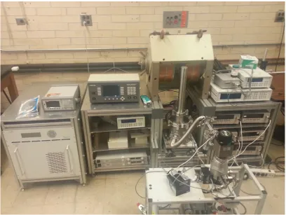
Figure 3.1. Nernst effect measuring system in our lab. ... 9
Figure 3.2. Sample lead diagram ... 10
Figure 3.3. Sample lead photograph ... 11
Figure 3.4. Connection schematic diagram ... 12
Figure 3.5. A sample mounted in the chamber. ... 13
Figure 4.1. Raw data for BiNiTe sample at constant temperature gradient. ... 19
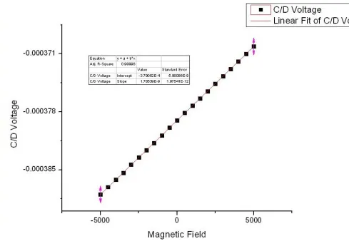
Figure 4.2. Plot of C/D Voltage vs. Magnetic Field for BiNiTe sample. ... 20
Figure 4.3. Plot of E/F Voltage vs. Magnetic Field for BiNiTe sample ... 21
Figure 4.4. Raw data for BiNiTe sample at constant magnetic field. ... 22
Figure 4.5. Plot of E/F Voltage vs. ∆T for BiNiTe sample at constant magnetic field. ... 22
Figure 4.6. Plot of C/D Voltage vs. ∆T for BiNiTe sample at constant magnetic field. ... 23
Figure 4.7. Raw data for BiSbTe sample at constant temperature gradient ... 25
Figure 4.8. Graph of E/F Voltage vs. Magnetic Field for BiSbTe sample. ... 26
Figure 4.9. Graph of C/D Voltage vs. Magnetic Field for BiSbTe sample. ... 27
Figure 4.10. Raw data for BiSbTe sample at constant magnetic field. ... 27
Figure 4.11. Plot of E/F Voltage vs. ∆T for BiSbTe sample. ... 28
Figure 4.12. Plot of C/D Voltage vs. ∆T for BiSbTe sample. ... 29
Figure 5.1. Misalignment in the voltage leads on the sample. ... 30
v
List of Tables
vi
Abstract
An experimental Nernst effect measuring system is designed and constructed. The ability to measure the Nernst effect allows completion of a thermoelectric suite of measurements
consisting of electrical conductivity, the Seebeck effect, the Hall effect, and the Nernst effect. This suite of measurements gives information about electron transport, carrier concentration, and electron scattering within a thermoelectric sample. Programs were designed in LabView to control the various instruments in the measuring system. Measurements of the Nernst effect were taken on two thermoelectric samples, bismuth nickel telluride and bismuth antimony telluride. These measurements were taken at both constant temperature and constant magnetic field. An error analysis of the Nernst effect measuring system is also presented, with consideration as to future work that can be done to improve the quality of Nernst effect measurements taken from the system.
1
Chapter 1.
Introduction
1.1. Introduction to Thermoelectric Materials
Thermoelectric materials are materials which have the ability to convert heat into electrical energy, or vice versa. Thermoelectric materials thus have many applications in power generation or refrigeration devices. The efficiency of a thermoelectric material is described by its figure of merit, Z, which is given by (Rowe, 2006)
1.1
where S is the Seebeck coefficient, σ is the electrical conductivity, and λ is the thermal
conductivity of the material. These coefficients and effects will be defined in greater detail in the following chapter. The quantity in the numerator of equation 1.1, S2σ, is often called the power factor. Multiplying Z by the absolute temperature, T, gives a dimensionless figure of merit, ZT. For practical applications, ZT must be larger than 1, and the best thermoelectric materials currently known have a ZT only slightly larger than 1.
1.2. Goals
2
Chapter 2.
Background Theory
2.1. Overview of Thermoelectric Effects
2.1.1. Electrical Conductivity
We open our discussion of thermoelectric effects with the simplest effect – that of electrical conductivity. Electrical conductivity (typically denoted by σ, although κ and γ are also used) represents the ability of a material to conduct electric current. Given a current density J and an electric field E, the electrical conductivity of the material is given as (Putley, 1960)
2.1
σ has units of Ampere/(Volt∙Meter). Amperes per volt is often defined as siemens in SI units or “mhos” in electrical applications.
Conductivity is the inverse of resistivity – the ability of a material to resist current flow. Resistivity is typically denoted by ρ and is defined as (Putley, 1960)
1
2.2
and has units of Ohm∙Meters.
2.1.2. The Seebeck Effect
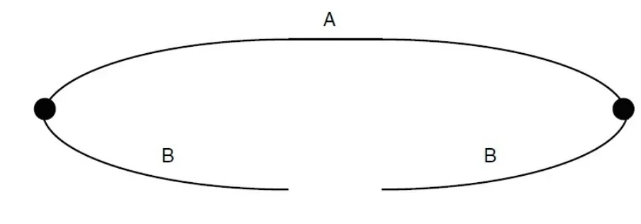
As previously mentioned, thermoelectric materials allow the conversion of heat into electrical energy. When a temperature gradient is applied to the material, an electric current will be produced. This process is known as the Seebeck Effect, discovered in 1821 by Thomas Johann Seebeck. The Seebeck effect is closely linked to thermocouples. A thermocouple is an electrical device consisting of two different conductors. These conductors are connected in series, but held at different temperatures T1 and T2. Under these conditions, a voltage V will
3
V ST T2.3
where S is the Seebeck coefficient. Solving for the Seebeck coefficient gives (Rowe, 2006)
S ΔT 2.4V
where ∆T is the temperature gradient T1-T2. S is positive if current flows in a clockwise direction
and is often on the order of µV/K.
Figure 2.1 A schematic of a simple thermocouple. "A" and "B" represent different materials. (Goldsmid, 2010)
2.1.3. The Peltier Effect
The Peltier Effect, named after French physicist Jean Charles Athanase Peltier who discovered it in 1834, is the inverse of the Seebeck Effect. If an external current source is applied between the two contacts of a thermocouple, heat will be generated between them. The Peltier coefficient, π, is defined as (Rowe, 2006)
2.5
4
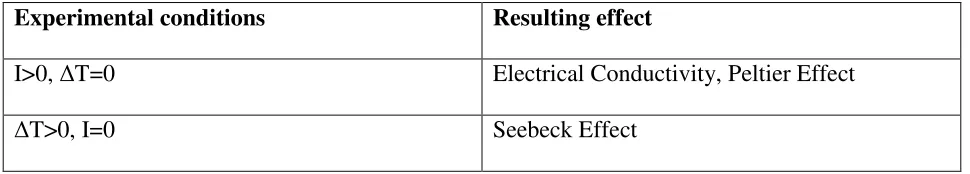
The following table serves to summarize the non-magnetic thermoelectric effects.
Table 2.1 A summary of the non-magnetic thermoelectric effects.
Experimental conditions Resulting effect
I>0, ∆T=0 Electrical Conductivity, Peltier Effect
∆T>0, I=0 Seebeck Effect
2.1.4. The Hall Effect
We begin discussion of the thermomagnetic effects with the Hall Effect. The Hall Effect, discovered in 1879 by Edwin Hall, allows us to determine the carrier type and concentration of carriers in a given sample. The Hall Effect is of particular importance in studying the Nernst Effect, as samples which give good Hall Effect measurements are ideal candidates for Nernst Effect measurements. The following derivation closely follows that in Sze and Ng Sze, 2007.
Consider electrons (or holes) flowing in the x direction in a sample. In the absence of a magnetic field, these electrons will follow nearly straight paths through the sample. If a magnetic field is applied in the z direction, the electrons will curve downward into the y direction and accumulate on one side of the sample, leaving an absence of charge on the opposite side. This curvature of electrons is due to the Lorentz force,
"# $% & '( 2.6
At steady-state, the Lorentz force will be exactly balanced by the electric field created in the y direction, Ey. That is,
"* "# 2.7
5
This electric field can be referred to as the Hall field. The Hall voltage (the voltage in the y direction) can thus be given as
-. +/ 2.9
where W is the width of the sample. We can also define the drift velocity of the electrons as
$% 12 2.10
where J is the current density, n is the carrier concentration, and e is the charge of the electron. J is defined as
3 2.11
where I is the current and A is the area of the sample. We thus can rewrite the drift velocity as
$% 312 2.12
and we can then rewrite the Hall voltage as
-. $%'(/ '312 (/ 412 2.13'(
where t is the thickness of the sample. We can also define the Hall coefficient as
5. '+ (
-.
/'(
-.3
/'(
-.4
'( 2.14
The sign of the Hall coefficient denotes the majority carriers in the sample. For electrons (n-type material) the Hall coefficient is negative, whereas for holes (p-type material) the Hall coefficient is positive. RH typically has units of m3/C but is occasionally expressed in different units such as Ω∙cm/G.
2.1.5. The Righi-Leduc Effect
6
gradient in the y direction, another temperature gradient will be produced in the x direction. The Righi-Leduc coefficient, A, is given as (Putley, 1960)
|3| 78:79
'(∙ 78 7;: 2.15
2.1.6. The Nernst Effect
The Nernst Effect can be viewed as thermally analogous to the Hall Effect. Where electrons are driven by the Lorentz force in the Hall Effect, electrons are also driven by the temperature gradient present in the Nernst Effect. Electrons will diffuse from the hot side of the sample to the cold side in order to establish thermal equilibrium. Thermoelectric materials exhibit the Nernst Effect when they are subjected to a magnetic field (Bz) and a temperature
gradient (dT/dx) at right angles to each other. Under these conditions, an electric field Ey will be
produced which is perpendicular to both the temperature gradient and the magnetic field. A relationship between these quantities can be expressed in the Nernst coefficient, N (Rowe, 2006):
|<| 78/7; 2.16+/'(
The Nernst effect is often referred to in literature as the First Nernst-Ettingshausen Effect, so named for its discoverers, Albert von Ettingshausen and his PhD student, Walther Nernst, who observed the effect in 1886 while studying the Hall Effect in Bismuth. Unlike the Hall Effect, the sign of N does not depend on the charge of the carriers in the material. N has units of V/(G∙K).
2.1.7. The Ettingshausen Effect
7
other, a temperature gradient will be produced perpendicular to both the magnetic and electric fields. This effect is quantified in the Ettingshausen coefficient, P (Rowe,2006):
|>| 78': ∙ 77; (
(? + 2.17
Where dz is the thickness of the sample and Iy is the current applied to the sample. P has units of
K/(G∙A).
There is a thermodynamic relationship between the Ettingshausen coefficient and the Nernst coefficient which can be expressed as (Goldsmid, 2010)
> <8 2.18
Here, as in equation 1.1, λ is the thermal conductivity. The thermal conductivity is included in the relationship since the Nernst and Ettingshausen effects are defined in terms of a temperature gradient rather than heat flow.
8
Figure 2.2. A visual summary of the thermomagnetic effects. Coefficients are positive when the effects are in the directions shown in the diagram (Goldsmid, 2010).
Table 2.2. A summary of the thermomagnetic effects. ∆T is the temperature difference, B is the magnetic field and I is electrical current.
Experimental Conditions Resulting Effect
∆T=0; B>0; I=0 Hall Effect
∆T>0; B>0; I=0 Nernst Effect, Righi-Leduc Effect
∆T=0; B>0; I>0. Ettingshausen Effect
Chapter 3.
Experimental Setup
3.1. Equipment
9
with a GMW System 8500 Magnet Power Supply in order to generate a magnetic field. This field is measured using a LakeShore 455 DSP Gaussmeter. We create a temperature gradient across the sample by powering a 100 Ω resistor attached to the sample to generate heat. This resistor is powered by a Kiethley 6221 AC/DC current source. We take voltage readings using Kiethley 2182A Nanovoltmeters. We use four nanovoltmeters total. Two of the nanovoltmeters are set up to read voltages across the sample. The other two nanovoltmeters take voltage readings from the thermocouples connected to the sample. We also use a Lakeshore 331S Temperature Controller to read the base temperature. All instruments are connected to the computer via GPIB, or General Purpose Information Bus. Connecting the instruments through GPIB allows programs such as LabView to interface with the instruments easily.
10 3.2. Sample Setup
Voltage leads are soldered directly to the sample as shown in the diagram below.
11
Figure 3.3. A photograph showing thermocouple and voltage leads attached to the sample.
12
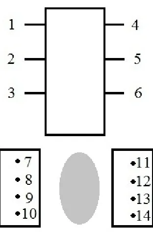
Figure 3.4. A schematic diagram showing how the sample is connected to the various measuring instruments. The gray oval represents the sample holder and thermocouple stage. The connections are as follows:
1: I+, KE6221 2: BNC “D” lead 3: BNC “C” lead 4: I-, KE6221
5: Top Thermocouple Copper (V1 +
) 6: BNC “A” lead
7: Top Thermocouple Constantan (V1-)
8: BNC “F” lead 9: BNC “E” lead 10: Empty 11: BNC “B” lead 12: Empty
13: Bottom Thermocouple Copper (V2 +
) 14: Bottom Thermocouple Constantan (V2-)
13
14
The BNC cables are connected to a converter box which we constructed in order to connect the BNC cables to the nanovoltmeters. The converter box also was designed with a slot for a 25-pin connector for connection to a LakeShore 370 AC Resistance Bridge. This allows us to make Hall Effect measurements in the future using the already existing system. The 25 pin connector will connect to BNC leads “A” and “B”, which are currently not used.
3.3. LabView Program Design
Before writing LabView programs to take measurements from the sample, it was necessary to design a program to control our electromagnet’s magnetic field. Designing this program proved to be a unique challenge. Our goal was to create a program that would allow the user to input a desired field and a tolerance, and quickly reach the inputted field. Both speed and precision are important – our measurements require a tolerance of 1 Gauss. A program was provided with the electromagnet, but we quickly realized that it was far too imprecise for our measurements. In addition, there was no way to automate this program, which would require us to manually set each field value, making measurements take a very long time. After studying the stock control program, we learned that the magnet is actually controlled by sending a current value to the electromagnet via GPIB. The magnet then passes that much current through it and produces a magnetic field accordingly. We took a graph of inputted current vs. outputted field and found a nearly linear relationship, with a small amount of hysteresis present in the
15
1) First, take a reading from the Gaussmeter to determine if the existing field is already within tolerance of the desired field. This serves as a sanity check and prevents us from wasting time trying to reach an already set field.
2) Next, we read the amount of current already being passed through the magnet. This determines our starting point.
3) Take a reading from the Gaussmeter and subtract the reading from the desired field. Dividing this by the slope of the line tells us how many additional amps of current need to be added in order to reach the desired field.
4) Add that much current to the current already present. Pass that amount of current. Take a reading from the Gaussmeter. If the reading is within tolerance, stop. If not, return to step 3.
This program works equally well for positive and negative field values. The magnet will automatically interpret negative current values as reversed polarity, eliminating the need to manually switch the magnet’s polarity. However, special care must be taken when trying to set the field to zero. The program requires longer waits in between steps when trying to reach zero, otherwise the magnet’s power supply will shut itself off. We believe this is caused by a bug in the power supply’s handling of small current values.
3.4. Taking Measurements
16
the temperature gradient, we vary the current, and thus, the power, supplied to the resistor on the sample. For example, a typical measurement profile would be from 22 mA to 28 mA, in 2 mA increments. Since > 5, where R= 100 Ω, the power supplied to the resistor ranges from 48.4 to 78.4 mW.
At each magnetic field or current value, we take a number of voltage readings (typically 20) from across the sample (C/D and E/F in Figure 2.2) and average them. We then record these averages in a text file, along with the standard deviation and variance for each reading. This process is then repeated for all magnetic field or current values. The data is then tabulated in Origin 8.0. We expect that plots of magnetic field or temperature gradient vs. C/D and E/F voltage will produce a straight line.
3.5. Approximations for the Nernst Coefficient
Additionally, we must relate the Nernst coefficient to the known and measured quantities we have. We previously defined the Nernst coefficient as (Rowe, 2006):
|<| 78/7; 2.16+/'(
We need to employ some algebraic manipulation in order to describe N in terms of our known quantities. First, we will approximate dT/dx as:
78
7; @ ∆8B 3.1
Here, l is the distance between the two thermocouples and ∆T=T2-T1, where T1 and T2
are the temperatures at the thermocouples. Since we cannot directly measure the temperatures at the thermocouples, we must again employ an approximation using the base temperature, T0, the
sensitivity at the base, S(T0), and the voltage measured from the thermocouples, V. We can thus
17 8 @ 8-
C D 8C3.2
8 @8-
C D 8C 3.3
Combining 2.2 and 2.3 gives an expression for ∆T:
∆8 8-
C D 8C
-
8C 8C
∆8 -8 -
C 3.4
We will also let E=V/d, where d is the thickness of the sample. Substituting into our expression for N gives:
< -/7'E8/B 7'∆8 3.5-B
If we are taking a measurement at constant temperature gradient (i.e., varying the magnetic field), the slope of the line plotted in Origin is:
FGHI -' 3.6
so our expression for N becomes:
< BF7∆8 3.7GHI
If we instead are taking measurements at constant magnetic field, the slope of the line is:
FJKGL ∆8 3.8
-and our expression for N is:
18
N is now completely in terms of known parameters: the thickness of the sample (d), the distance between thermocouples (l), the magnetic field strength (B), the temperature difference between the two thermocouples (∆T), and the voltage (V).
Chapter 4.
Results
We measured two different samples in order to test our measuring system: bismuth nickel telluride (BiNiTe) and bismuth antimony telluride (BiSbTe). We measured each sample at both constant temperature and at constant magnetic field. Results for each sample are listed in the following tables. Raw data and graphs for BiNiTe at constant temperature gradient follows:
Magnetic Field (G) E/F Voltage (V) C/D Voltage (V) Bot TC Volt (V) Top TC Volt (V)
19
Figure 4.1. Raw data for BiNiTe sample at constant temperature gradient. Note: Bot TC Temp and Top TC Temp values are the temperature difference from the base temperature, not the absolute temperature at the thermocouple. LabView carries out this calculation autom
Current Level (mA): 25
Base Temperature (K): 2.968200E+2 Sample TC Length (mm): 5.6222 Sample Thickness (mm): 2.44
Average Bottom Temperature Difference (K): 9.17918 Average Top Temperature Difference (K): 19.7594 Temperature Gradient across sample (K/mm): 1.88186
Bot TC Temp (K) Top TC Temp (K) E/F Std. Dev. C/D Std. Dev Bot TC Volt S.Dev Top TC Volt S.Dev
9.18148 19.74423 7.36088E-09 1.63787E-08 2.67474E-09 6.30359E-09
9.18105 19.74518 7.13477E-09 8.04861E-09 3.32941E-09 4.63078E-09
9.18044 19.74584 1.04673E-08 2.27347E-08 3.93667E-09 3.30917E-09
9.18013 19.74667 1.01242E-08 2.35184E-08 2.26804E-09 7.35335E-09
9.18032 19.74862 9.09288E-09 5.54190E-09 2.98171E-09 7.81865E-09
9.18066 19.75096 2.26565E-08 2.25838E-08 2.27495E-09 1.15804E-08
9.18162 19.75408 1.95194E-08 2.89690E-08 3.92680E-09 1.00266E-08
9.18242 19.75734 2.20386E-08 1.77580E-08 1.94140E-09 1.03291E-08
9.18259 19.75971 1.89738E-08 1.49314E-08 1.43065E-09 7.38828E-09
9.18236 19.76125 8.81285E-09 1.48472E-08 3.13079E-09 1.96369E-09
9.18133 19.76177 3.10906E-08 8.80664E-09 1.34668E-09 7.59526E-09
9.18141 19.76444 6.96927E-09 1.90104E-08 3.21239E-09 8.55880E-09
9.18140 19.76643 1.11154E-08 9.12973E-09 2.23914E-09 4.83699E-09
9.18148 19.76852 1.25650E-08 1.45521E-08 3.50829E-09 7.16641E-09
9.18053 19.76905 3.04623E-08 6.76748E-09 7.64242E-09 2.33880E-09
9.17900 19.76904 1.19045E-08 1.05973E-08 5.75594E-09 3.10762E-09
9.17752 19.76915 1.37534E-08 1.36950E-08 5.43965E-09 2.29926E-09
9.17653 19.76998 1.05893E-08 5.54475E-09 8.53890E-09 3.94580E-09
9.17411 19.76859 2.17142E-08 7.36793E-09 1.25408E-08 8.79799E-09
9.17076 19.76554 2.33446E-08 1.45795E-08 1.58085E-08 1.88983E-08
20
21
Figure 4.3. Plot of E/F Voltage vs. Magnetic Field for BiNiTe sample
Using equation 3.7 and using the E/F slope gives a Nernst coefficient of 2.6714&10-10 V/(K∙G), or 2.6714&10-6 V/(K∙T). The same calculation using the C/D slope instead gives a Nernst coefficient of 3.8881&10-10 V/(K∙G), or 3.881&10-6 V/(K∙T).
22
Figure 4.4. Raw data for BiNiTe sample at constant magnetic field.
Magnetic Field: 5000 G = 0.5 T Base Temperature (K): 296.8200 Sample TC Length (mm): 5.6222 Sample Thickness (mm): 2.44
Figure 4.5. Plot of E/F Voltage vs. ∆T for BiNiTe sample at constant 5000G field.
Current (mA) E/F Voltage (V) C/D Voltage (V) Top TC Voltage (V) Bot TC Voltage (V) E/F Volt S. Dev C/D Volt S. Dev
22 1.27E-04 -2.98E-04 6.18E-04 2.87E-04 1.65E-08 7.98E-08
24 1.49E-04 -3.46E-04 7.38E-04 3.43E-04 5.39E-08 5.78E-08
26 1.74E-04 -3.94E-04 8.69E-04 4.05E-04 5.68E-08 6.35E-08
28 1.99E-04 -4.42E-04 0.00101 4.71E-04 1.70E-08 5.37E-08
Top TC Volt S. Dev Bot TC Volt S. Dev Top Delta T(K) Bot Delta T(K) Base Temp(K) Delta T (K) Temp Gradient (K/mm)
4.30E-07 2.80E-07 15.19458 7.04637 296.77 8.14821 1.44934402
4.32E-07 2.86E-07 18.1422 8.43144 296.8 9.71076 1.72727825
4.64E-07 3.10E-07 21.34574 9.94052 296.83 11.40522 2.02867714
23
Figure 4.6. Plot of C/D Voltage vs. ∆T for BiNiTe sample at 5000G magnetic field.
It is important to note in Figure 3.6 that, although the voltage is becoming more negative, the magnitude of the voltage is the important quantity. The magnitude of the voltage is
increasing with increasing temperature gradient, which agrees with theory.
Using equation 3.9and the E/F slope gives a Nernst coefficient of 6.5713*10-9 V/(K∙G), or 6.5713∙10-5 V/(K∙T). Using the C/D slope gives a coefficient of 1.3027*10-8 V/(K∙G), or 1.3027∙10-4 V/(K∙T).
24
Magnetic Field (G) E/F Voltage (V) C/D Voltage (V) Bot TC Voltage (V) Top TC Voltage (V) Bot TC Temp (K) Top TC Temp (K)
5000.20 -3.68E-04 -8.79E-05 1.87E-04 1.10E-03 4.57E+00 2.71E+01
4499.70 -3.68E-04 -8.69E-05 1.87E-04 1.10E-03 4.57E+00 2.71E+01
3999.60 -3.67E-04 -8.56E-05 1.87E-04 1.10E-03 4.57E+00 2.71E+01
3499.10 -3.66E-04 -8.60E-05 1.87E-04 1.10E-03 4.57E+00 2.71E+01
2999.70 -3.66E-04 -8.60E-05 1.87E-04 1.10E-03 4.57E+00 2.71E+01
2499.50 -3.65E-04 -8.53E-05 1.87E-04 1.10E-03 4.57E+00 2.71E+01
1999.80 -3.65E-04 -8.41E-05 1.87E-04 1.10E-03 4.57E+00 2.71E+01
1499.45 -3.64E-04 -8.37E-05 1.87E-04 1.10E-03 4.57E+00 2.71E+01
999.42 -3.63E-04 -8.29E-05 1.87E-04 1.10E-03 4.57E+00 2.71E+01
499.40 -3.63E-04 -8.25E-05 1.87E-04 1.10E-03 4.57E+00 2.71E+01
0.69 -3.63E-04 -8.30E-05 1.87E-04 1.10E-03 4.57E+00 2.71E+01
-500.72 -3.62E-04 -8.14E-05 1.87E-04 1.10E-03 4.57E+00 2.71E+01
-1000.82 -3.62E-04 -8.04E-05 1.86E-04 1.10E-03 4.57E+00 2.71E+01
-1500.97 -3.61E-04 -8.01E-05 1.86E-04 1.10E-03 4.57E+00 2.70E+01
-2000.98 -3.60E-04 -7.94E-05 1.86E-04 1.10E-03 4.57E+00 2.70E+01
-2500.26 -3.60E-04 -7.87E-05 1.87E-04 1.10E-03 4.57E+00 2.70E+01
-3000.60 -3.59E-04 -7.77E-05 1.87E-04 1.10E-03 4.57E+00 2.71E+01
-3500.70 -3.59E-04 -7.71E-05 1.87E-04 1.10E-03 4.57E+00 2.71E+01
-4000.10 -3.58E-04 -7.59E-05 1.87E-04 1.10E-03 4.57E+00 2.70E+01
-4500.80 -3.58E-04 -7.55E-05 1.87E-04 1.10E-03 4.57E+00 2.70E+01
25
Figure 4.7. Raw data for BiSbTe sample at constant temperature gradient
Current Level (mA): 25 Base Temperature(K): 298.35 Current Level (mA): 25
Sample TC Length (mm): 6.7858 Sample Thickness (mm): 2.38 Average Bot Temperature Difference (K): 4.57 Average Top Temperature Difference (K): 27.1
Temperature Gradient across sample: 3.3135 K/mm
E/F Std. Dev. C/D Std. Dev Bot TC Volt S.Dev Top TC Volt S.Dev
7.12E-09 9.32E-08 5.75E-09 1.89E-08
1.42E-08 2.37E-07 3.49E-09 1.08E-08
1.59E-08 1.35E-07 2.38E-09 3.29E-09
9.05E-09 1.76E-07 6.64E-09 1.72E-08
5.09E-09 1.39E-07 4.00E-09 1.19E-08
1.51E-08 1.61E-07 3.01E-09 1.32E-08
1.08E-08 2.56E-07 2.20E-09 4.59E-09
1.67E-08 1.19E-07 1.97E-09 5.83E-09
1.95E-08 1.09E-07 5.87E-09 1.81E-08
1.31E-08 1.85E-07 2.98E-09 1.04E-08
1.27E-08 4.12E-07 7.64E-09 4.01E-08
9.48E-09 1.23E-07 4.31E-09 6.97E-09
1.35E-08 2.36E-07 9.33E-09 2.31E-08
9.41E-09 2.15E-07 4.78E-09 1.70E-08
1.02E-08 1.82E-07 1.05E-09 3.21E-09
9.08E-09 1.39E-07 4.99E-09 9.68E-09
1.25E-08 1.04E-07 2.25E-09 2.86E-09
9.15E-09 1.98E-07 4.71E-09 1.23E-08
1.41E-08 3.19E-07 2.23E-09 2.76E-09
9.50E-09 1.14E-07 1.52E-09 3.61E-09
26
27
Figure 4.9. Graph of C/D Voltage vs. Magnetic Field for BiSbTe sample.
Using equation 3.7and using the E/F Slope gives a Nernst coefficient of 1.4101&10-10 V/(G∙K), or 1.4101&10-6 V/(T∙K). Using the C/D Slope instead gives a Nernst coefficient of 1.6234&10-10 V/(G∙K), or 1.6234&10-6 V/(T∙K).
Raw data and graphs for BiSbTe sample at constant magnetic field follows.
Figure 4.10. Raw data for BiSbTe sample at constant magnetic field.
Current (mA) E/F Voltage (V) C/D Voltage (V) Top TC Voltage (V) Bot TC Voltage (V) E/F Volt S. Dev C/D Volt S. Dev
22.00 -2.82E-04 -6.90E-05 8.57E-04 1.47E-04 1.82E-07 3.85E-07
24.00 -3.35E-04 -8.29E-05 1.02E-03 1.74E-04 2.36E-07 2.48E-07
26.00 -3.91E-04 -1.00E-04 1.20E-03 2.04E-04 2.52E-07 1.69E-07
28.00 -4.53E-04 -1.18E-04 1.39E-03 2.35E-04 2.60E-07 3.73E-07
Top TC Volt S. Dev Bot TC Volt S. Dev Top Delta T(K) Bot Delta T(K) Base Temp(K) Delta T (K) Temperature Gradient (K/mm)
6.31E-07 1.60E-07 21.01 3.60 2.98E+02 17.41 2.565677326
6.49E-07 1.66E-07 25.03 4.27 2.98E+02 20.76 3.059532597
7.09E-07 1.77E-07 29.40 4.99 2.98E+02 24.41 3.5970663
28
Magnetic Field: 5000 G = 0.5 T Base Temperature (K): 298.00 Sample TC Length (mm): 6.7858 Sample Thickness (mm): 2.38
29
Figure 4.12. Plot of C/D Voltage vs. ∆T for BiSbTe sample.
Using equation 3.9and using the E/F Slope gives a Nernst coefficient of 8.888&10-9 V/(G∙K), or 8.888×10⁻⁵ V/(T∙K). Using the C/D Slope instead gives a Nernst coefficient of 2.5655×10⁻⁹ V/(G*K), or 2.5655×10⁻⁵ V/(T*K).
Chapter 5.
Discussion
5.1. Improvement of Results
30
Figure 5.1. Misalignment in the voltage leads on the sample.
31
5.1.1. Error Analysis
In order to verify that the misalignment is the major source of error in our experimental setup, we took an error analysis of our experimental parameters using equation (3.5).
< 7'∆8 -B
The total error of our experiment will be given by
8M4NB OOMO PQ∆-- QD Q∆BB QD Q∆77 QD Q∆88 QD Q∆'' Q 5.1
Calculations for each term of equation 5.1 follow. Values for BiNiTe sample will be used. To calculate the error in the voltage, we will use the average E/F voltage values and take the average standard deviation for these values:
Q∆-- Q 1.59723 ∙ 101.56823 ∙ 10RSRT 1.0185 ∙ 10RT5.2
In calculating the error for l, the distance between the thermocouples, we measured the spot size of the BiNiTe sample to be 0.833 mm. We can determine the location of each wire to approximately half the spot size, or 0.4167 mm.
Q∆BB Q 6.1278 5.29445.7111 0.1459 5.3
Error for d, the thickness of the sample, was calculated by taking a thickness measurement at both the top and the bottom of the sample. The sample is not perfectly rectangular and this will introduce a small error into the measurement.
Q∆77 Q 2.48 2.442.44 0.0164 5.4
32
values are tabulated by NIST for type T thermocouples by listing values of thermocouple EMF for different temperature values. Values are listed from -270 °C to 400 °C. The following graph shows values at 20 °C.
Figure 5.2. Graph of Temperature vs. Thermocouple EMF. The sensitivity value at 20 °C is 0.0405 mV/°C.
We calculated sensitivity values at given temperatures by linear fit of temperature vs. EMF values. The LabView program simply looks up the nearest sensitivity value for a given base temperature. The sensitivity values vary by approximately 6% over a 10 °C range, so the error in sensitivity measurements could be as large as 6%.
Magnetic field measurements are taken in 500 Gauss steps and are accurate within a tolerance of 1 Gauss.
Q∆'' Q 500 4 ∙ 101 RU5.5
Substituting the results from equations 5.2-5.5 and figure 5.2 into equation 5.1 gives a total error of 0.1586, or 15.86%. As expected, the thermocouple distance term is the majority of
y = 0.0405x - 0.0203 R² = 0.9999
0.740 0.750 0.760 0.770 0.780 0.790 0.800 0.810 0.820 0.830 0.840
18 19 20 21 22
E M F ( m V ) TEMPERATURE (C)
Type T Thermocouple
Type T
33
the source of error in our measurements. 15% of the distance between the thermocouples is approximately half a millimeter. Assuming a temperature gradient of 3 K/mm, this results in a 1.5 K error. If we assume a Seebeck coefficient of 250 µV/K, this error produces a voltage of up to 375 µV, which is many orders of magnitude larger than the Nernst voltage.
The following table serves to summarize our error analysis.
Term Error % Error (Error · 100%)
V 1.02·10-4 1.02·10-2%
l 0.15 15%
d 0.016 1.6%
T 0.06 6%
B 4·10-6 4·10-4%
Table 5.1. Summary of errors for terms in equation 3.5.
5.1.2. Improvements to Experimental Setup
We first thought to use silver paste as an adhesive for the voltage leads rather than soldering the leads directly on the sample. Silver paste is an extremely conductive adhesive and is much easier to work with than solder, so aligning the leads would be much simpler for one to do. However, voltage readings with silver paste instead of solder were extremely poor and thus silver paste proved to not be a viable solution to the misalignment problem.
One solution proposed for the misalignment problem is the construction of a small, rotating sample holder. The holder would allow rotation of the sample in all three directions and would make it possible to precisely solder voltage leads onto the sample.
34
Chapter 6.
Conclusions
35
Bibliography
R. Bel et al. Giant Nernst Effect in CeCoIn5. Physical Review Letters, Volume 92, Number 21.
2004.
H. Julian Goldsmid. Introduction to Thermoelectricity. Springer-Verlag, 2010. E.H. Putley. The Hall Effect and Related Phenomena. Butterworth and Co. 1960. D.M. Rowe. Thermoelectrics Handbook: Macro to Nano. CRC Press, 2006.
36