Volume 12 - Article 3 | Pages 51–76

in the population sciences published by the Max Planck Institute for Demographic Research Konrad-Zuse Str. 1, D-18057 Rostock · GERMANY www.demographic-research.org

DEMOGRAPHIC RESEARCH

VOLUME 12, ARTICLE 3, PAGES 51-76

PUBLISHED 10 MARCH 2005

www.demographic-research.org/Volumes/Vol12/3

DOI: 10.4054/DemRes.2005.12.3

Research Article

Intrinsically dynamic population models

Robert Schoen

1 Introduction 52 2 The two age group Intrinsically Dynamic Model 53

2.1 Analyzing Leslie Matrices 53

2.2 The Constant Subordinate Eigenstructure approach 55

3 The three age group IDM 59

4 The n age group IDM 63

5 IDM dynamics 64

5.1 The IDM birth trajectory 64

5.2 Observed populations as IDM populations 65 5.3 Transitions between stable population regimes 67 5.4 Momentum following a gradual or irregular decline

to zero growth

69

6 Summary and conclusions 71

References 72

Intrinsically dynamic population models

Robert Schoen1

Abstract

Intrinsically dynamic models (IDMs) depict populations whose cumulative growth rate over a number of intervals is equal to the product of the long term growth rates (that is the dominant roots or dominant eigenvalues) associated with each of those intervals. Here the focus is on the birth trajectory produced by a sequence of population projection (Leslie) matrices. The elements of a Leslie matrix are represented as straightforward functions of the roots of the matrix, and new relationships are presented linking the roots of a matrix to its Net Reproduction Rate and stable mean age of childbearing. Incorporating mortality changes in the rates of reproduction yields IDMs when the subordinate roots are held constant over time. In IDMs, the birth trajectory generated by any specified sequence of Leslie matrices can be found analytically.

In the Leslie model with 15 year age groups, the constant subordinate root assump-tion leads to reasonable changes in the age pattern of fertility, and equaassump-tions (27) and (30) provide the population size and structure that result from changing levels of net reproduc-tion. IDMs generalize the fixed rate stable model. They can characterize any observed population, and can provide new insights into dynamic demographic behavior, including the momentum associated with gradual or irregular paths to zero growth.

1_{Department of Sociology, Pennsylvania State University, 211 Oswald Tower, University Park PA 16802}

1. Introduction

For nearly a century, Lotka’s stable population has been the central model of mathematical demography. In a stable population, time invariant age-specific rates of birth and death produce an exponentially increasing sequence of births and an unchanging age structure (cf. Lotka 1939; Keyfitz 1968). In the 1940s, the discrete form of Lotka’s continuous model was investigated, and the power of matrix theory brought to bear (Leslie 1945; Pollard 1973). Since the 1970s, the model has been extended to the multistate case, where more than one living state and the movements between them are recognized (Land and Rogers 1982; Rogers 1975; Schoen 1988). Yet the stable approach demands fixed vital rates. In a rapidly changing world characterized by numerous short term fluctuations and uncertain long term trends, a fixed rate assumption is unrealistic and often untenable.

To move beyond stable population constraints, demographers have sought to develop dynamic models, i.e. models with changing vital rates. In a pioneering work, Coale (1972) investigated patterns of dynamic rates and found approximate relationships be-tween changing rates and the birth sequences they produced; closed form expressions eluded him. Lee (1974) considered dynamics in populations subject to external con-straints. Preston and Coale (1982), building on Bennett and Horiuchi (1981), found closed form relationships that characterized any population, though they did not explicitly incor-porate dynamics. Kim (1987) analyzed discrete dynamic models and found a general algebraic solution connecting changing rates and their birth sequences. However, in most instances, her solution was too complex to render in closed form. Cyclically stable pop-ulations, which arise when a fixed sequence of rates repeat indefinitely, have also been examined (Tuljapurkar 1990; Caswell 2001). An explicit solution can be found for a se-quence of two rate schedules in a population with two reproductive age groups (Schoen and Kim 1994a), but most cyclical populations are far too complex for direct algebraic solution.

Recent work on “hyperstable” models has related given birth trajectories to a consis-tent underlying set of vital rates (Schoen and Kim 1994b; Kim and Schoen 1996) or to a sequence of fertility levels (Schoen and Kim 1997). Schoen and Jonsson (2003) pre-sented a modified form of Quadratic Hyperstable (QH) model that related monotonically increasing (or decreasing) fertility rates to an exponentiated quadratic birth sequence. The QH model provides closed form relationships that generalize the stable model, but the QH model is limited to one specific type of monotonic change in fertility.

2. The two age group Intrinsically Dynamic Model

2.1 Analyzing Leslie Matrices

To lay the foundation for the approach presented here, we begin with a brief review of the structure of population projection matrices (PPMs). A more complete treatment can be found in Caswell (2001) and the references cited there.

Consider a 2 age group population projection (Leslie) matrix that projects the begin-ning of the interval population to the end of the interval, i.e.

A=

a b

1 0

. (1)

The first row elements, a and b, indicate the contribution of the first and second age groups, respectively, at the beginning of the interval to the number of persons in the first age group at the beginning of the next interval. The first element of the second row, 1, indicates that all persons in the first age group at the beginning of the interval survive to be in the second age group at the beginning of the next interval. Our focus here is on the birth trajectory, rather than on the age structure, and the form ofAgenerates successive numbers of births. In effect, we assume that mortality is incorporated in the “fertility” rates in the first row of A, and by combining mortality with fertility we simplify the structure of the Leslie matrices.

Now let the initial population be described by the vector

x0=

x10

x20

(2)

wherex_jtdenotes the number of persons in thejth age group at timet. We then have the projection relationship

x1=Ax0 (3)

where the elements ofx₁are the “births” (i.e. numbers in the first age group) at times 1 and 0.

Any matrix can be expressed in terms of its eigenvalues and eigenvectors (Caswell 2001). Doing so provides a mathematical decomposition of the matrix, but one with substantive interpretations in demographic usage. Accordingly, we can write

A=UΛV . (4)

rates of the two ”components” implicit in matrixA. Eigenvalueλ₁, the dominant root, describes the rate of growth of the dominant (stable) component, and must be greater thanλ₂, the growth rate of the subordinate component (cf. Keyfitz 1968). In terms of Lotka’s intrinsic rate of natural increase,r, we have the relationshipλ₁ = emr, where mis the number of years in the projection interval. (In the 2 age group case,m = 25.) The eigenvalues are defined by the characteristic equation|A−λI| = 0, whereIis the identity matrix (here of order 2) and the vertical lines denote the determinant. With the characteristic equation ofAgiven by

−λ(a−λ)−b= 0 (5)

we have the eigenvalues

λ= 1₂a±(a2_{+ 4b)}1 2

(6)

where the dominant eigenvalue is provided by the positive root in equation (6).

MatrixUis the matrix of right eigenvectors, and by convention is written in the form

U =

1 1

u1 u2

. (7)

In Leslie matrices, the right eigenvectors describe the age composition of the compo-nents. Specifically,u₁is the number of persons in the second age group relative to a unit number in the first age group in the stable population that arises from the persistence of PPMA. All of the elements of the first (dominant component) right eigenvector must be real and non-negative, and it is the only right eigenvector with those properties. In the

2×2Leslie matrix,u₂, which reflects the age structure of the subordinate component, is real but always negative. Given the form ofAin equation (1), we can write (Caswell 2001)

u1=λ−11;u2=λ−21; (8)

whereλ₂<0.

MatrixV = U−1 is the matrix of left eigenvectors. Substantively, they reflect the present value of future births in each component ofA, where those births are discounted over time by the eigenvalue of that component. The first row of V relates to the first (dominant, or stable population) component. Elements in the first column give repro-ductive values for the first age group and those in the second column for the second age group. Given equation (1), we have

V =

1 −λ2

−λ2

λ1 λ2

λ1

(λ1−λ2)

The mean age of childbearing implied by matrixA, µ_A, is given by

a λ1

+2b λ2 1

. In

terms of roots,µ_A= (λ1_λ−λ2)

1 , the reciprocal of the scalar expression in curly brackets on the right of equation (9).

Convergence to stability occurs asAis raised to higher powers (i.e. as the initial pop-ulation is projected further into the future). The matrixAp, the product ofAmultiplied by itselfptimes, can be seen as equal toUΛpV. Becauseλ₂< λ₁, λp₂becomes insignif-icant in comparison withλp₁as p becomes large. After a sufficiently long period, sayP intervals, λP₂ can be considered zero,APand becomes a “rank one” matrix, i.e. becomes equal toλP₁ times the product of the first column ofU and the first row ofV (Caswell 2001; for a thorough discussion of the process of convergence, see Keyfitz 1968.)

2.2 The Constant Subordinate Eigenstructure approach

To specify an analytically useful dynamic model, we need to find an algebraic expression for the product of a sequence of Leslie matrices when those matrices are changing over time. That is a difficult problem because matrix multiplication is generally not commuta-tive. As a result, the desired product generally cannot be written in closed form, but only as a product integral which must be evaluated numerically (cf. Gantmacher 1959).

To obtain a special case where the product of PPMs is analytically tractable, we seek an appropriate simplifying assumption. An appealing possibility is to have the growth rate over a number of intervals equal the product of the growth rates of each of those intervals. That greatly simplifies the specification of the birth sequence in terms of the fertility rates of each interval, the crucial relationship we seek to determine. Tuljapurkar (1990: 83-85) noted that when Leslie matrices shared a common set of reproductive values, overall growth equaled the product of the λ₁’s of the individual matrices. Schoen (2003) ex-amined multistate models with uniform natural increase across model states, and found population projection matrices that had both that multiplicative property in the growth rates and constant relative reproductive values. In Leslie matrices with no mortality, like those of equation (1), equation (8) shows that an eigenvalue constant over time has an eigenvector that is constant over time. Accordingly, let us consider Leslie matrices where only the dominant eigenvalue varies over time, while the subordinate eigenvalue(s) re-main constant. A sequence of such Leslie matrices should have the desired multiplicative property in the growth rates.

can thus be written as

At=

λ1t+λ2 −λ1tλ2

1 0

(10)

where the time (t) subscript has been added to dominant rootλ₁. Using equation (6), it can readily be verified thata_t = λ_1t+λ₂,b_t =−λ_1tλ₂andλ_1tandλ₂are the eigen-values ofA_t. Subordinate roots are not commonly encountered in demographic work, though the ratio λ2

λ1 is related to the rate of convergence to stability (Kim and Schoen 1993). However, equation (10) shows that the elements of our base Leslie matrix can be expressed as simple, symmetric functions of the dominant and subordinate roots. While that relationship is not new, its implications for demographic analysis have not been ap-preciated.

Now consider the productM_0,2 = A₂A₁. In terms of its own eigenstructure, the product matrixM_0,2can be written in the form of equation (4) as

M0,2=UM2ΛM2VM2 (11)

and we find that

UM2=

_{1 1}

λ11+λ2

λ11(λ12+λ2)

1

λ2

(12)

ΛM2=

λ12λ11 0

0 λ2 2

(13)

and

VM2=

_{1 −λ}

2

−λ2(λ11+λ2)

λ11(λ12+λ2) λ2

λ11(λ12+λ2)

λ12λ11−λ22)

. (14)

Paralleling equation (9), we denote the scalar factor on the right side of equation (14) as

1/µM2.

Because of the constant subordinate eigenvector restriction, that product has three important properties (Gantmacher 1959). First, the desired multiplicative property holds: the eigenvalues ofM_0,2are equal to the products of the eigenvalues ofA₁andA₂. Thus the sequence of PPMsA₂A₁can be termed “intrinsically dynamic” in the sense that their product matrix (M) grows at a rate that is equal to the product of their individual growth rates.

Third, the relative sizes of the first row elements of the left eigenvector matrices of all three PPMs are equal. However, the scalar factor associated with V_M2 (that can be interpreted as reflecting the reciprocal of the mean age at childbearing) does vary over time.

The dominant right eigenvector ofM is not constant, allowing the age composition of the dynamic model to change over time. To determine how it changes in the long term, consider the situation at time P, when only the dominant component of the dynamic population remains. The form of equations (11)-(14) indicates that the rank one product matrix,M_0,P, can be written in terms of its dominant root, its dominant right (column) eigenvector, and its dominant left (row) eigenvector as

M0,P = P

j=1

λ1j

₁

µMP 1

λ1PµM,P−1

(1−λ2). (15)

Equation (15) incorporates the scalar mean age at childbearing into the column vector, leaving the row vector constant. Let element (i, j) be the element in theith row andjth column of a matrix. At timeP, the (1,1) element ofM is the product of thePdominant eigenvalues times the factor1/µ_MP. The (2,1) element of M at timePis the (1,1) element of M at timeP−1, i.e. the product of the first(P−1)λ₁’s times1/µ_M,P−1. Accordingly, the ratio of the second age group to the first at timeP (that is the (2,1) element ofU_MP) is given by

µMP

(λ1PµM,P−1).

Equation (15) gives the size and structure of the long term “intrinsically dynamic model” (IDM) in terms of known PPM roots and the still to be determined mean age functionµ_Mt. To findµ_Mt, note that the form of the column vector in equation (15) and the known constant subordinate eigenvector allow us to write

UMt=

1 1

µMt

λ1tµM,t−1

1

λ2

. (16)

Because, at all times,V =U−1, equation (16) can be used to findV_Mt, and show that the scalar factor ofV_Mtis

1

µMt =

λ1t

λ1t−λ2

µMt

µM,t−1

. (17)

Rewriting equation (17), we have the recursive relationship

1

µMt =

λ1t+_µM,tλ2₋₁

at every timet. Combining equation (18) for timest, t−1, t−2, and so on to eliminate µM values at times beforetgives the solution

1

µMt = 1 +

λ2

λ1t+

λ2 2

λ1tλ1,t−1 +

λ3 2

λ1tλ1,t−1λ1,t−2+

λ4 2

λ1tλ1,t−1λ1,t−2λ1,t−3 +. . . .

(19) The infinite series in equation (19) must converge because its terms alternate in sign (asλ₂ <0) and the absolute value of the ratioλ₂/λ_1tis always less than 1 (sinceλ_1tis the dominant root). Straightforward algebra confirms that equations (15) and (19) satisfy the long term IDM projection equation

xt=Atxt−1 (20)

whenx_tandx_t−1are equated to the product of theλ₁’s times the column vector given in equation (15), andA_tis given by equation (10). In the stable case, whereλ₁is constant, the series in equation (19) sums toλ₁/(λ₁−λ₂), the scalar factor _µ1

A in equation (9).

[see Appendix note 1]

Heuristically, as time passes, equation (19) shows how a one time increase inλ₁is steadily diminished by being relegated to successively smaller, higher order terms un-til its effect disappears. It follows that _µ1

Mt increases, or the product matrix mean age

at childbearing decreases, wheneverλ_1trises. Fundamentally, equation (19) reconciles population growth byλ_1tbetween timest−1andtwith the population’s legacy of past growth at different rates, growth which leaves its imprint in the population’s age compo-sition. The birth cohort size adjustments that follow from equation (19) make the long term “intrinsic dynamics” of the model possible.

The solution for the 2 age group IDM in equations (15) and (19) was verified by com-parison with calculations on hypothetical data using the mathematical package Maple. Table 1 compares the product matrix with values calculated from equations (15) and (19). In the calculations,λ_1t= 1 +.04tandλ₂=−0.4. Those values implya_t=.6 +.04t andb_t=.4 +.016t. The Net Reproduction Rate (NRR) at timet,R_t, is the sum ofa_t andb_tor1 +.2t. After 12 projection intervals (300 years), the product matrix is close to rank one asλ12₂ =.0000168. By projection, mean ageµ_M,12 = 1.26871(in units of 25 years). Table 1 shows five different theoretically calculated values, where the series in equation (19) is followed to consecutively higher powers ofλ₂. Convergence occurs fairly quickly, with 6 terms of the series (150 years) providing accuracy to about.002and 9 terms to about.0001.

Table 1: Comparison of Two Age Group Intrinsically Dynamic Model Values From Equations (15) and (19) With Those From a Population Projection

Product matrix Product matrix element from summing element from the series up toλ2terms of the power

population

projection 5 6 7 8 9

Age group (j)

1 11.73411 11.72737 11.73626 11.73339 11.73435 11.73402 2 7.88256 7.87718 7.88435 7.88196 7.88279 7.88249

Note: Population projection matrix (At) specified byλ1t= 1 +.04tandλ2=−0.4.Values shown refer to the

(j,1) element of the time 12 product matrix.

3. The three age group IDM

Let our 3 age group, time varying Leslie matrix,A_t, be given by

At=



 a₁t b_{0 0}t ct

0 1 0



 (21)

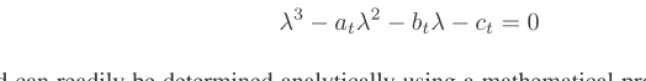
where again we assume that mortality is included in the first row elements and our pro-jection follows the birth trajectory. The eigenvectors of PPM A_t are the roots of the characteristic equation (cf. Pollard 1973)

λ3_−a

tλ2−btλ−ct= 0 (22)

and can readily be determined analytically using a mathematical program like Maple or Mathematica. [see Appendix note 2] Tuljapurkar (1993: 265) showed that the net ma-ternity values of any Leslie matrix can be written in terms of its eigenvalues. Using that relationship,A_tcan be written

At=



 λ1t+λ₁2+λ3 −(λ1tλ2+λ₀1tλ3+λ2λ3) λ1tλ₀2λ3

0 1 0



 (23)

where we again assume that onlyλ₁varies with time.

Aτis

Uτ =

   

1 1 1

λ−_1τ1 λ−₂1 λ−₃1 λ−_1τ2 λ−₂2 λ−₃2

  

 . (24)

The inverse ofUτ yields the left eigenvector matrix

Vτ =

     

1 −(λ2+λ3) λ2λ3

−λ2

2(λ1τ−λ3)

λ2

1τ(λ2−λ3)

λ2

2(λ21τ−λ23)

λ2

1τ(λ2−λ3)

−λ2

2λ1τλ3(λ1τ−λ3)

λ2

1τ(λ2−λ3)

λ2

3(λ1τ−λ2)

λ2

1τ(λ2−λ3)

−λ2

3(λ21τ−λ22)

λ2

1τ(λ2−λ3)

λ2

3λ1τλ2(λ1τ−λ2)

λ2

1τ(λ2−λ3)

      1 µAτ (25)

where the mean age of childbearing implied byA_τ,µ_Aτ, is given by

µAτ= (λ1τ−λ2_λ)(₂λ1τ−λ3)

1τ .

(26)

Using the structure of the eigenvectors ofA_τ and the reasoning underlying equation (15), we can write the long term product matrix as

M0,t=

  

t

j=1

λ1j

       1 µMt 1 (λ1tµM,t−1)

1 (λ1tλ1,t−1µM,t−2)

  

(1 −(λ2+λ3) λ2λ3). (27)

The (1,1) element ofM_0,tis the product of the individual PPM growth rates, divided byµ_Mt; the (2,1) element is the product of the PPMs up to timet−1, divided byµ_M,t−1; and the (3,1) element is the product of the PPMs up to timet−2, divided byµ_M,t−2. The latter two elements are simply the (1,1) elements ofM at times t−1andt−2, respectively. The row vector of relative reproductive values remains fixed over time and equal to its stable population counterpart.

To findµ_Mt, we note that with constant subordinate eigenvectors the fullU_Mtmatrix can be written

UMt=

   

1 1 1

µMt

(λ1tµM,t−1) λ

−1 2 λ−31

µMt

(λ1tλ1,t−1µM,t−2) λ

−2 2 λ−32

  

Using the relationshipV_Mt=U_Mt−1and equating the scalar factor associated with the first row ofV_Mtto1/µ_Mtyields the recursive relationship

1

µMt = 1 +

(λ2+λ3)

λ1tµM,t−1 −

(λ2λ3)

λ1tλ1,t−1µM,t−2 . (29)

Using the relationship in equation (29) to eliminateµ_M at times before t leads to_µ1

Mt

as the sum of the series

1

µMt = 1 +

(λ2+λ3)

λ1t +

(λ3

2−λ33)

(λ2−λ3)

(λ1tλ1,t−1)+

+

(λ4

2−λ43)

(λ2−λ3)

(λ1tλ1,t−1λ1,t−2)+

(λ5

2−λ53)

(λ2−λ3)

(λ1tλ1,t−1λ1,t−2λ1,t−3)+. . . (30)

Equations (27) and (30) provide the basic relationships underlying the 3 age group IDM. The infinite series in equation (30) converges because it is an alternating series and λ1t>−(λ2+λ3), sinceλ_1t+λ₂+λ₃=a_t>0. Equations (23), (27), and (30) satisfy basic projection equation (20), confirming the solution. Those equations apply regardless of whether the two subordinate roots are real and unequal, real and equal, or complex conjugates.

Table 2 compares the projected product matrix with values calculated from equations (27) and (30). In the calculations,λ_1t= 1 +.02t,λ₂=−.2, andλ₃ =−.5. The NRR at any time can be found by summing the first row elements of theA_tmatrix in equation (21). Algebraically, that yields

Rt= 1−(1−λ1t)(1−λ2)(1−λ3). (31)

With the present values,R_t= 1 +.036t, indicating how the NRR increases linearly with time (andλ_1t). After 20 projection intervals (300 years, as 3 age groups imply 15 year intervals), the product matrix is very close to rank one;λ20₂ is less than.000001. In the projection, mean age µ_M,20 = 1.54841(in units of 15 years). Table 2 shows four theoretically calculated values, where the series in equation (30) is summed over the first 7 through 10 terms. Convergence is a bit slower (in terms of number of intervals) than in the two age group case. Differences between projected and calculated values are about .01−.02after 7 terms of the series, and about.001after 10 terms (150 years).

Table 2: Comparison of Three Age Group Intrinsically Dynamic Model Values From Equations (27) and (30) With Those From a Population Projection

Product matrix Product matrix element from equations element from (27) and (30), summing the series to term number population projection 7 8 9 10 Age group (j)

1 26.67127 26.65159 26.67917 26.66805 26.67261 2 18.94539 18.92959 18.95184 18.94272 18.94652 3 13.65055 13.63766 13.65589 13.64830 13.65152

Note: Population projection matrix (At) specified byλ1t= 1 +.02t,λ2=−.2andλ3=−.5. Values shown

refer to the (j,1) element of the time 20 product matrix.

roots, and Pattern 3 a double root. Those four patterns span the most commonly found three age group discrete fertility schedules (Schoen and Kim 1996).

Table 3: Fertility Patterns and Their Variation With the Dominant Root in 3 Age Group Intrinsically Dynamic Models

Pattern 1 Pattern 2 Pattern 3 Pattern 4

Root (λ1) a b c a b c a b c a b c

.8 .2 .38 .08 .1 .46 .08 0 .48 .128 0 .44 .16 .9 .3 .44 .09 .2 .53 .09 .1 .56 .144 .1 .52 .18 1.0 .4 .5 .1 .3 .6 .1 .2 .64 .16 .2 .6 .2 1.1 .5 .56 .11 .4 .67 .11 .3 .72 .176 .3 .68 .22 1.2 .6 .62 .12 .5 .74 .12 .4 .80 .192 .4 .76 .24 1.3 .7 .68 .13 .6 .81 .13 .5 .88 .208 .5 .84 .26 1.4 .8 .74 .14 .7 .88 .14 .6 .96 .224 .6 .92 .28 1.5 .9 .80 .15 .8 .95 .15 .7 1.04 .24 .7 1.00 .30 Subordinate roots −.3±.1i −.2,−.5 −.4(double root) −.4±.2i

and down, values ofλ₁below.8would lead to unacceptable (negative) fertility values. The constant subordinate eigenstructure assumption was chosen for its mathematical, not its demographic, properties. By restricting the age pattern of fertility, it permits any pattern of change in fertility levels over time and allows the resultant birth trajectory to be found (and, with a mortality assumption, gives the age composition of the population at any time). The ability to vary the level of fertility represents a substantial extension of the stable population model, and at the price of an assumption that is no more unrealistic than fixed rates. The IDM first row PPM elements are all linear functions ofλ₁, and hence of each other, and need not reproduce (or approximate) the characteristic age pattern of fertility. Yet they generally produce reasonable values over a broad range of λvalues when there are three reproductive ages. While investigators using IDMs need to verify that acceptable age patterns of fertility exist, Table 3 suggests that it is usually possible to do so.

4. The n age group IDM

To extend the intrinsically dynamic model to the case ofnage groups, let our standard form Leslie matrixA_thave first row elementsa_jt,j= 1, . . . , n. As before, the subdiag-onal elements are equal to 1. The characteristic equation ofA_tis then

λn

t −a1tλn−t 1−a2tλn−t 2−. . .−ant= 0. (32)

From the relationship between roots and coefficients in polynomial equations, then coefficients can be written in terms of thenroots of equation (32). Specifically,a_1tis the sum of the roots taken one at a time;a_2tis minus the sum of the roots taken 2 at a time; anda_jtis(−1)j+1 times the sum of the roots takenjat a time. As a result, in the IDM all of thea_jtare linear functions ofλ_1t.

In Leslie matrixA_t, several basic demographic measures are expressible as relatively simple functions of allnroots. Summing the first row elements of the matrix and rear-ranging terms gives the NRR as

Rt= 1−

n

j=1

(1−λjt). (33)

In intrinsically dynamic models, the NRR is always a linear function of λ₁ (and vice versa).

The mean age of childbearing implied byA_tcan be defined by the relationship

µAt= a_λ1t

1t+ 2a2t

λ2

1t +. . .+

nant

λn

1t .

Rewriting that relationship in terms of roots yields

µAt=λ11−nt

n

j=2

(λ1t−λj). (35)

The approach used in the 2 and 3 age group models can generate the product matrix andµ_Mtin thenage group case. Once again, thejth root of the product matrix is the product of thejth roots of the individual PPMs. Apart from the µ_Mt factor and with one as the first element, thejth element in the first row of the left eigenvector matrix is

(−1)j−1_{times the sum of the subordinate roots takenj−1at a time. The first column of}

the right eigenvector matrix has first term1/µ_Mt, andjth term

1

[µM,t−j+1(λ1j)] ,

where the product goes fromt−j+2tot. A recursive equation for mean ageµ_Mtcan be found by extending equation (28) to specify the first column ofU_Mt, usingV_Mt =U_Mt−1, and then equating the scalar factor ofV_Mtto1/µ_Mt. Asnbecomes large, the expressions get quite complicated.

Beyond complexity, there is a serious problem with thenage group IDM as a vehicle for analyzing human populations. The pattern of fertility change required by the constant subordinate eigenstructure assumption becomes increasingly inappropriate whenn ≥4. Consider the conventional Leslie matrix with 10 five-year age groups. Since human popu-lations have essentially zero fertility below age 10, the (1,1) element of that Leslie matrix must be zero. However, any change in the dominant root would cause the (1,1) element to change by an equal amount, producing a PPM with unrealistic or unacceptable values. Consequently, the focus here is on the 3 age group model. Table 3 shows that the age patterns of fertility are quite reasonable in that model, and 15 year age groups coincide closely with the typical beginning of reproduction, the mean age of childbearing, and the end of reproduction. Moreover, it is not difficult to condense a 10 age group Leslie matrix to 3 groups (Keyfitz 1968, p37-40).

5. IDM Dynamics

5.1 The IDM birth trajectory

Consider the case whereλ_1t=eht, for some known constanth. Since

t

j=1

hj=ht(t+ 1)₂ ,

we have

λMt= exp(ht(t₂+ 1)). (36)

Using different assumptions, Schoen and Kim (1997) and Schoen and Jonsson (2003) also found exponentiated quadratic growth associated with exponentially increasing net reproduction. Other polynomial functions forλ_1talso lead to exponentiated growth in births at an order one degree higher than the largest power of t in λ_1t. For example, Maple calculations indicate that ifλ_1t= exp(ht2), thenλ_Mt = exp(ht(t+1)(2₆ t+1)), and ifλ_1t= exp(ht3), thenλ_Mt= exp(ht2(t₄+1)2).

The ability to analyze cyclical fluctuations in fertility is particularly useful, and si-nusoidal patterns inλ_1tcan be summed analytically. In particular, Maple computations show that

t

j=1

sinωj=1₂sinω−sinω(t+ 1) + (cotω₂){sinωcosω−cosω(t+ 1)} . (37)

Schoen and Kim (1997) found a similar expression for cyclical net reproduction by assuming a constant generation length, though their approach did not provide any underly-ing age-specific birth rates. Under polynomial growth inλ_1t, the relative size adjustments produced by the1/µ_Mtfactor may be small, as they were in the case of the linearly in-creasingλ_1tof Table 2. With cyclical changes, however, those adjustments may play a much larger role.

5.2 Observed populations as IDM populations

Any observed population distribution can be viewed as an IDM population distribution. That representation is not unique, however, as different intrinsically dynamic models fol-low from alternative assumptions regarding the (constant) subordinate roots and the nature of the past birth trajectory.

restore the birth sequence, we can write

x0=

  _x1₂₀

x30



 (38)

wherex_j0 represents the number of persons in thejth age group at initial time 0. To simplify the calculations, assume that the population was stable with dominant growth rateλ_Aand subordinate rootsλ₂ andλ₃before time (−1). Then, from the definition of λAand equation (26)

λA = x_x20

30

µA = (λA−λ2_λ)(₂λA−λ3)

A .

(39)

To specify the IDM, we need to find the time 0 cumulative growth rate (λ_M0) and the time 0 product matrix mean age at childbearing (µ_M0). Using equation (27), with the scale readjusted so that the population age 0-14 is 1, we can equate the second element of the scaled column vector with the second element in the population in equation (38) and write

x20= _(µµM0

AλM0) . (40)

Using equations (30) and (39), we can replace the infinite series in equation (30) with the stableµ_Aand show that

1

µM0 = 1−

λA

λM0(1−_µ1_A).

(41)

Combining equations (40) and (41) yields the solutions

λM0 = 1 +x20_xλA(µA−1) 20µA

µM0 = 1 +x20λA(µA−1). (42)

With equation (42), the IDM representation can be written as

x0=

   

1

[λA+µA(λM0−λA)]−1 [λ2

A+λAµA(λM0−λA)]−1

  

The form of equation (43) makes it clear that the age composition becomes that of the λAstable population whenλA=λM0.

To illustrate the procedure numerically, letx₀’=[1 .6 .4], where the prime (’) indicates the vector transpose. Assuming stability before time (−1) and setting λ₂ = −.2 and λ3 = −.5, we findλ_A = 1.5,µ_A = 1.51111, λ_M0 = 1.61029, and µ_M0 = 1.46, with age and time in units of 15 years. The faster pace of growth from time (−1) to 0 (λ₀ = 1/.6 = 1.66667), compared toλ_A = 1.5between times (−2) and (−1), leads to an increase in cumulative growth from1.5to1.61029and a fall in the (implicit) product matrix mean age at childbearing from1.51111to1.46.

5.3 Transitions between stable population regimes

Intrinsically dynamic models can be used to examine transitions from one set of fixed rates to another. If a stable population growing atλ_Awere suddenly to shift to a regime with long term growth atλ_B, the subordinate roots remaining constant, its dynamics would be that of an IDM.

Consider a 3 reproductive age group model, and let the number of persons under age 15 at time 0 be scaled to 1. With the change in regimes fromλ_Atoλ_Boccurring at time 0, equations (27) and (30) describe the subsequent behavior of the population. Table 4 and Figure 1 show the birth trajectory (i.e. the number of persons under age 15) when λA = 1.5andλ_B = 1under two different patterns of fertility, specifically Patterns 2 and 4 of Table 3. After the fall in fertility to replacement level, the number of births falls sharply, then recovers some, and eventually approaches its ultimate stationary level. When all of theλ₁values in equation (30) are the same, equation (26 ) applies. With the initial number of births scaled to 1, equation (27) indicates that the ultimate birth level is

µA

µB. Table 4 and Figure 2 show howµMtmoves fromµAtoµB along a path similar to

that of the birth trajectory. Consistent with Preston (1986) and Kim and Schoen (1997), the number of persons under age 30 remains quite level during the transition.

The concept of population momentum, introduced in Keyfitz (1971), refers to the increase in population size that accompanies the transition to zero growth. Given a drop to replacement level fertility at a specified initial time, momentum,Ω, is the ratio of the total size of the ultimate stationary population to the total size of the initial population. Mathematically, it can be written (cf. Schoen and Jonsson 2003)

Ω =be0Q (44)

Figure 1: The Birth Trajectory Following a Transition, at Time 0, From a Stable (λ_A= 1.5) to a Stationary (λ_B= 1) Regime, Under Two Fertility Patterns

-20 30 80 130 180 230 280

Time (t) 0.6

0.7 0.8 0.9 1.0

Population Age 0-14

∞

Figure 2: The Cumulative Mean Age of Childbearing (µ_Mt) Following a Transition, at Time 0, From a Stable (λ_A= 1.5) to a Stationary (λ_B = 1) Regime, Under Two Fertility Patterns

-20 30 80 130 180 230 280

Time (t) 21

23 25 27 29 31 33 35 37

µ

M t

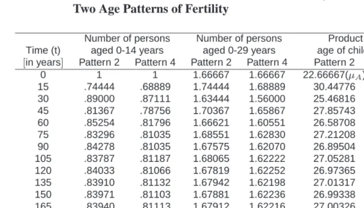
Table 4: The Birth Trajectory and Related Measures Following a Transition, at Time 0, From a Stable (λ_A=1.5) to a Stationary (λ_B=1) Regime, Under Two Age Patterns of Fertility

Number of persons Number of persons Product matrix mean Time (t) aged 0-14 years aged 0-29 years age of childbearing (µMt)

[in years] Pattern 2 Pattern 4 Pattern 2 Pattern 4 Pattern 2 Pattern 4 0 1 1 1.66667 1.66667 22.66667(µA) 24.33333 (µA) 15 .74444 .68889 1.74444 1.68889 30.44776 35.32258 30 .89000 .87111 1.63444 1.56000 25.46816 27.93367 45 .81367 .78756 1.70367 1.65867 27.85743 30.89729 60 .85254 .81796 1.66621 1.60551 26.58708 29.74897 75 .83296 .81035 1.68551 1.62830 27.21208 30.02830 90 .84278 .81035 1.67575 1.62070 26.89504 30.02804 105 .83787 .81187 1.68065 1.62222 27.05281 29.97196 120 .84033 .81066 1.67819 1.62252 26.97365 30.01686 135 .83910 .81132 1.67942 1.62198 27.01317 29.99213 150 .83971 .81103 1.67881 1.62236 26.99338 30.00292 165 .83940 .81113 1.67912 1.62216 27.00326 29.99922 180 .83956 .81111 1.67896 1.62224 26.99829 30.00001 195 .83948 .81111 1.67904 1.62222 27.00073 30.00011 210 .83952 .81111 1.67901 1.62222 26.99945 29.99986 225 .83951 .81111 1.67903 1.62222 27.00000 30.00001 240 .83952 .81111 1.67903 1.62222 26.99959 29.99990

∞ .83951 .81111 1.67901 1.62222 27.00000(µB) 30.00000(µB)

Note: Equation (30) is summed through the16th_{term. Under Fertility Pattern 2,λ}

2=−.2andλ3=−.5. Under Fertility Pattern 4,λ2=−.4 +.2iandλ3=−.4−.2i.

initial birth cohort. As indicated above, in the IDM

Q=_µµA

B . (45)

When fertility falls, the mean age at childbearing in an IDM rises. The ratio of initial to ultimate mean ages of childbearing mirrors the ratio of initial to ultimate birth cohort sizes.

5.4 Momentum following a gradual or irregular decline to zero growth

That relationship, made applicable to any initial population by equation (42), means that the IDM context can be used to examine the population growth associated with any arbitrary route to stationarity. The subject has received considerable attention recently for several reasons. Substantively, Bongaarts and Bulatao (1999) found that momen-tum effects are likely to account for most of the future growth in the world’s popula-tion. Analytically, Schoen and Kim (1998), Li and Tuljapurkar (1999; 2000), Goldstein (2002), Goldstein and Stecklov (2002), and Schoen and Jonsson (2003) have extended techniques for finding momentum under a variety of paths to zero growth. That work has demonstrated the dramatic increases in ultimate population size that result from delays in achieving zero growth. All of those approaches, however, are either approximate, impose substantial constraints on the length or pattern of decline, or both.

Equation (27) can yield exact solutions for essentially any path to zero growth in terms of initial mean ageµ_M0, ultimate stationary mean ageµ_B, and the product of the nonstationary PPM growth rates between initial time 0 and the time,B, when the rates attain their final stationary level. Mathematically, withQ∗ denoting the relative size of the ultimate birth cohort,

Q∗₌

  

B

j=1

λ1j

  

µM0

µB . (46)

In the intrinsically dynamic population, ultimate birth cohort size is determined by the product of individual PPM intrinsic growth rates, modified only by the initial and ultimate product matrix mean ages at childbearing. Momentum follows immediately from equation (44).

Table 5 compares population momentum values from equations (44) and (46) with those from population projections under a range of assumptions about the length and pattern of fertility decline. The initial population is the IDM withλ₁ = 1.5,λ₂ =−.2, andλ₃ = −.5, which has an NRR of1.90. Under contemporary conditions, the value ofbe₀ for that population is approximately 2, and that value is used in the calculations. Two different patterns of decline over time are considered, one linear with respect to the NRR, and the other linear with respect toλ₁. One projection is done assuming a linear (proportional) decline over age, and the other assuming that the pattern of decline keeps the subordinate eigenvalues constant.

Table 5: Population Momentum Associated With Different Routes to

Stationarity, Calculated By Population Projections and By Equations (44) and (46)

Linear Decline in NRR Over Time Linear Decline in PPMλ1Over Time Years Before

Zero Growth From Projection From Projection

Attained Linear decline IDM decline From IDM Linear decline IDM decline From IDM over age over age equation (46) over age over age equation (46) 0 1.714 1.679 1.679 1.714 1.679 1.679 15 2.143 2.099 2.099 2.128 2.099 2.099 30 2.678 2.612 2.612 2.645 2.612 2.612 45 3.344 3.247 3.247 3.285 3.247 3.247

Note: Initial population stable atλ1= 1.5with NRR= 1.90. IDM subordinate roots areλ2=−.2andλ3=−.5.

In all models, the product of the initial birth rate and the ultimate life expectancy is set at 2.

case of linear NRR declines. Because that NRR/growth relationship does not hold when fertility changes proportionally over all ages, the linear decline in λ₁ projections yield slightly different results from the linear decline in NRR projections. The rather modest effect associated with different age patterns of fertility decline can be seen as enhancing the value of equations (44) and (46), as it suggests that the age pattern required by the constant subordinate root assumption has only a small effect on momentum. In addition to validating the analytical results presented, Table 5 shows how delays in attaining zero growth greatly increase momentum. In the case considered, the population would grow from1to1.7if stationary rates were achieved immediately, but would grow to over3.2if the decline took place over 45 years.

6. Summary and conclusions

Intrinsically dynamic models, based on an assumption of constant subordinate roots, have been developed to provide a new approach to analyzing populations with changing rates. Because of the constraints on the age pattern of fertility associated with that assumption, attention is focused on the discrete (Leslie) model with 15 year age intervals. Equations (27) and (30) provide a complete solution for the population produced by any time pattern of change in the level of fertility (or in period-by-period growth levels).

References

Bennett, N.G. and S. Horiuchi. (1981). Estimating the completeness of death registration in a closed population. Population Index, 47, 207-21.

Birkhoff, G. and S. MacLane. (1959). A survey of modern algebra (rev. ed). New York: Macmillan.

Bongaarts, J. and R.A. Bulatao. (1999). Completing the demographic transition.

Popula-tion and Development Review, 25, 515-29.

Caswell, H. (2001). Matrix population models (2d ed). Sunderland MA: Sinauer.

Coale, A.J. (1972). The growth and structure of human populations. Princeton: Princeton University Press.

Gantmacher, F.R. (1959). Matrix theory. New York: Chelsea.

Goldstein, J.R. (2002). Population momentum for gradual demographic transitions: An alternative approach. Demography, 39, 65-73.

Goldstein, J.R. and G. Stecklov. (2002). Long-range population projections made simple.

Population and Development Review, 28, 121-41.

Keyfitz, N. (1968). Introduction to the mathematics of population. Reading MA: Addison-Wesley.

Keyfitz, N. (1971). On the momentum of population growth. Demography, 8, 71-80.

Kim, Y.J. (1987). Dynamics of populations with changing rates: Generalization of stable population theory. Theoretical Population Biology, 31, 306-22.

Kim, Y.J. and R. Schoen. (1993). On the intrinsic force of convergence to stability.

Mathematical Population Studies, 4, 89-102.

Kim, Y.J. and R. Schoen. (1996). Populations with quadratic exponential growth.

Math-ematical Population Studies, 6, 19-33.

Kim, Y.J. and R. Schoen. (1997). Population momentum expresses population aging.

Demography, 34, 421-27.

Lee, R. (1974). The formal dynamics of controlled populations and the echo, the boom, and the bust. Demography, 11, 563-85.

Leslie, P.H. (1945). On the use of matrices in certain population mathematics. Biometrika,

33, 183-212.

Li, N. and S. Tuljapurkar. (1999). Population momentum for gradual demographic tran-sitions. Population Studies, 53, 255-62.

Li, N. and S. Tuljapurkar. (2000). The solution of time-dependent population models.

Mathematical Population Studies, 7, 311-29.

Lotka, A.J. (1939). Theorie analytique des associations biologiques. Paris: Hermann.

Pollard, J.H. (1973). Mathematical models for the growth of human populations. Cam-bridge: Cambridge University Press.

Preston, S.H. (1986). The relation between actual and intrinsic growth rates. Population

Studies, 40, 495-501.

Preston, S.H. and A.J. Coale. (1982). Age structure, growth, attrition, and accession: A new synthesis. Population Index, 48, 217-59.

Rogers, A. (1975). Introduction to multiregional mathematical demography. New York: Wiley.

Schoen, R. (1988). Modeling multigroup populations. New York: Plenum.

Schoen, R. (2003). Dynamic populations with uniform natural increase across states.

Mathematical Population Studies, 10, 195-210.

Schoen, R. and S.H. Jonsson. (2003). Modeling momentum in gradual demographic transitions. Demography, 40, 621-35.

Schoen, R. and Y.J. Kim. (1994a). Cyclically stable populations. Mathematical

Popula-tion Studies, 4, 283-95.

Schoen, R. and Y.J. Kim. (1994b). Hyperstability. Paper presented at the Annual Meeting

of the Population Association of America, Miami, May 5-7.

Schoen, R. and Y.J. Kim. (1996). Stabilization, birth waves, and the surge in the elderly.

Schoen, R. and Y.J. Kim. (1997). Exploring cyclic net reproduction. Mathematical

Population Studies, 6, 277-90.

Schoen, R. and Y.J. Kim. (1998). Momentum under a gradual approach to zero growth.

Population Studies, 52, 295-99.

Tuljapurkar, S. (1990). Population dynamics in variable environments (Vol. 85). New York: Springer.

Tuljapurkar, S.D. (1993). Entropy and convergence in dynamics and demography.

Jour-nal of Mathematical Biology, 31, 253-71.

Appendix

1. In some cases, the series in equation (19) can be summed algebraically. For example, if

λ1,t−τ = _{λ_{1 +}0{1 +_bsinbsin_ω[tω₋[t_τ−₋τ_1]]}_}

Maple summation finds that(_µ1

Mt)is of the form

1

µMt

= 1 +C1t+C2tsinωt+C3tcosωt

where C_1t = λ2

(λ0−λ2)(1 +bsinωt)

C2t = _(λ2 bλ2(λ2−λ0cosω)

2−2λ0λ2cosω+λ20)(1 +bsinωt)

and C_3t = −bλ0λ2(sinω)

(λ2

2−2λ0λ2cosω+λ20)(1 +bsinωt).

2. The cubic characteristic equation of the 3 age group Leslie matrix given in equation (22) has the roots

λ1 = [2a+Z+

(12b+4a2₎

Z ] 6

λ2 = [4a−Z−

(12b+4a2₎

Z ]

12 + (

√

3i

12 )[Z−

(12b+ 4a2₎

Z ]

λ3 = [4a−Z−

(12b+4a2₎

Z ]

12 −(

√

3i

12 )[Z−

(12b+ 4a2₎

Z ] where