A b s t r a c t. Multisensor capacitance probes (MCPs) have been used in many soil water-related fields. The manufacturer re-commends a site-specific calibration before MCP use, and the cali-bration protocol requires replicated measurements of soil water content and MCP readings in the same soil volumes. In field re-search, such calibration is hardly plausible, and results cannot be extrapolated to plot average water contents in heterogeneous soils. A site-specific correction of the manufacturer calibration is a pra-ctical alternative to the field calibration in this case.
The Typic Hapludult soil at the OPE3 USDA-ARS research site in Beltsville, MD was sampled in triplicate at the distance of 50 cm from four MCPs on three dates with distinctly different water contents. Both systematic and random differences between MCP and plot-average gravimetrically determined water contents were encountered. The manufacturer calibration led to the overesti-mation of low water contents and to the underestioveresti-mation of high water contents. The depth-specific linear transformation of the factory calibration improved the estimation of plot-average water contents at all observation depths. Correcting MCP measurements for depth resulted in up to a 14.6% decrease in root-mean-square difference between MCP and plot-average measurements. Site-specific calibration correction may be useful when using MCPs in soil water monitoring.
K e y w o r d s: water content, multisensor capacitance probes, site-specific correction
INTRODUCTION
Multisensor capacitance probes (MCPs) are widely used in field soil water content measurements (Fareset al., 2006; Paltineanu and Starr, 2000; Starr and Paltineanu, 1998).
They have been used in irrigation scheduling (Fares and Polyakov, 2006), estimating soil hydraulic properties (Kelleners et al., 2005), evaluating tree water uptake (Schaffner, 1998) and other applications. The MCPs are pro-vided with a factory calibration, which establishes a rela-tionship between water content and scaled frequency mea-sured in soil. The manufacturer’s manual (Calibration of SENTEK Pty Ltd Soil Moisture Sensors, 2001) recom-mends to perform soil- or site-specific calibration of MCPs. Soil-specific MCP calibrations have been obtained under laboratory conditions (Baumhardtet al., 2000; Evettet al., 2006; Mead et al., 1995; Paltineanu and Starr, 1997; Polyakovet al., 2005) and field environments (Fareset al., 2004; Morganet al., 1999; Polyakovet al., 2005). Those studies showed that the MCP calibration could be adequately described by two- and three-parameter power equations, with soil- and depth-specific parameters.
The calibration protocol (Calibration of SENTEK Pty Ltd. Soil Moisture Sensors, 2001) requires replicated mea-surements of soil water content and MCP readings in the same soil volumes. The EnviroSCAN response volume is approximately within 3 cm distance from the access tube (Paltineanu and Starr, 1997). Taking samples in such close proximity to access tube is complex and time- and labor-consuming procedure that makes the field calibration plot unsuitable for further research. This may be critical for either short term or long term studies sensitive to soil distur-bance in close proximity to the sensor. As an alternative to the field calibration, a solution could be found in the cor-rection of the existing calibration equations. The corcor-rection would consists of establishing a relationship between water
Field correction of the multisensor capacitance probe calibration**
A.K. Guber
1*, Y.A. Pachepsky
1, R. Rowland
1, and T.J. Gish
21USDA-ARS Environmental Microbial and Food Safety Laboratory, Bldg 173 Powder Mill Road, BARC-EAST, Beltsville, MD 20705, USA
2USDA-ARS Hydrology and Remote Sensing Laboratory, 10300 Baltimore Avenue, Bldg 007, BARC-WEST, Beltsville MD 20705, USA
Received November 16, 2009; accepted November 30, 2009
© 2010 Institute of Agrophysics, Polish Academy of Sciences *Corresponding author’s e-mail: Andrey.Guber@ars.usda.gov
**This work was partially funded by NRC/USDA Interagency Agreement IAA-NRC-05-005 on ‘Model Abstraction Techniques to Simulate Transport in Soils’.
A
A
Agggrrroooppphhyhyysssiiicccsss
contents calculated from scaled frequencies using an existing MCP calibration and water contents in samples taken outside of the sensor installation zone at the sensor installation depth. The corrected water content measure-ments would reflect the average water contents across the sampling area rather than water contents in the small zone around the sensor. Since soil samples would be taken beyond the sensor installation, the disturbance around the MCP access tube would be minimized and the plot could then be used for water flow and chemical transport studies.
MCP calibration corrections may not be needed in ideal homogeneous soil layers. However in heterogeneous soils, the average water content across relatively small areas can be influenced by structural, textural and other heteroge-neities that are not detected by the sensor with a small acqui-sition volume.
The objectives of this work were to evaluate the need for MCP calibration correction across 1m2plots of a hetero-geneous coarse-textural soil and to develop a simple corre-ction procedure if necessary.
MATERIALS AND METHODS
The research site was part of the Optimizing Production inputs for Economic and Environmental Enhancement (OPE3) research site located at the USDA-ARS Beltsville Agricultural Research Center, Beltsville, Maryland (39°01’ 00" N, 76°52’00" W). Soil at this site has been classified as a coarse-loamy, siliceous, mesic Typic Hapludult with either well or excessively well drainage. A typical profile in-cludes a coarse sandy loam surface horizon (0-25 cm, organic matter 1.2-5.1%), a sandy clay loam horizon (25-100 cm), and a loam horizon below 140 cm, with loamy sand and fine textured clay loam lenses between 120 and 250 cm. Multi-sensor capacitance probes (EnviroSCAN, SENTEK Pty Ltd., South Australia) were installed in spring of 2006 to monitor soil water content and provide data for validation of a water flow model.Four plots (each 1 m2and 10 m apart) were instrumented with MCPs. The sensors were centered at 10, 20, 30, 40, 50, and 60 cm depths. Each sensor was norma-lized in air and water before installation. Undisturbed 98 cm3 soil cores were taken with a soil sample ring kit (Eijkelkamp Agrisearch Equipment BV, Giesbeek, the Netherlands) at a distance of 50 cm from the MCPs in the vertices of an equilateral triangle in triplicate at three dates with distinctly different water contents from depths corresponding to the MCPs installation. The triangle was rotated by 45°before
the second and third sampling. The holes made by sampling were refilled and compacted to prevent preferential water flow. Soil water content and soil bulk density were measured gravimetrically in the samples to derive volumetric soil water content. Soil texture was measured with the pipette method (Gee and Or, 2002) after dispersion with sodium pyrophosphate Na4P2O7in the soil samples taken as MCP access tubes were installed.
To compare MCP measurements with observed water content, the sensor scaled frequency (SF) was converted to volumetric water content using the SENTEK (1995) factory calibration equation:
q= (0.792SF– 0.0226)2.4752, (1)
and the laboratory calibration for mesic Aquic Hapludult silt loam soil (Paltineanu and Starr, 1997):
q= 0.490SF2.1674. (2)
The root-mean-square difference (RMSD) between plot-averaged and MCP-estimated water content was used to characterize the MCP measurements.
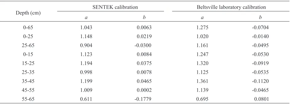
To correct the MCP measurements, the coefficientsa andbof linear regression between MCP-measured (è) and plot-averaged (q) water contents were calculated:
q=aq+b. (3)
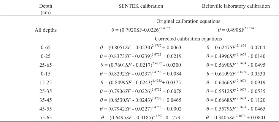
The coefficientacorrected the slope, and coefficientb corrected the bias of the SENTEK factory and the original laboratory calibration curves. Finally, the corrected calibra-tions were derived combining Eq. (3) with Eq. (1) and Eq. (2). The corrections were applied for data from all depths pooled together, for the topsoil (0-25 cm) data, for subsoil (25-65 cm) data and for each observation depth separately.
RESULTS AND DISCUSSION
Substantial variability in soil texture and soil bulk density with depth was observed at the four locations (Tables 1, 2). Generally clay content was less in the topsoil (0-25 cm) than in the subsoil (25-65 cm) layer. Silt content was relatively constant (17-25%) at all depths, while sand content was less in the subsoil compared to the content in the topsoil. Soil bulk density was less in the topsoil (1.34-1.69 g cm-3) than in the subsoil (1.69-1.95 g cm-3). The variation coefficient of soil bulk density ranged from 1 to 14%.
Depth (cm)
Clay Silt Sand
(%)
0-15 15 ± 6* 24 ± 9 61 ± 4
15-25 17 ± 4 23 ± 7 60 ± 3
25-35 22 ± 3 22 ± 5 56 ± 7
35-45 23 ± 4 21 ± 4 56 ± 7
45-55 24 ± 4 22 ± 4 54 ± 6
55-65 21 ± 6 21 ± 3 58 ± 2
*± separates the average from the standard deviation.
T a b l e 1.Soil texture at locations of the multisensor capacitance
Soil samples were taken at three dates when the soil was not excessively hard or soft for sampling, resulting in diffe-rent soil water content ranges at diffediffe-rent soil depths. Gene-rally, the water content range was wider in the top layer com-pared to that in the subsurface layers. Soil water contents were in the range from 0.103 to 0.510 m3m-3in the topsoil, from 0.090 to 0.422 m3m-3at depths of 25-55 cm, and from 0.090 to 0.376 m3m-3in the soil layer 55-65 cm of the four plots (Fig. 1). Spatial variability in the soil water content measured at each of the four plots changed with soil depth. Minimum (0.009 m3m-3) and maximum (0.032 m3m-3) plot averaged standard deviations of the water content were observed at 10, and 60 cm depths, respectively. At depths from 20 to 50 cm the standard deviations ranged from 0.024 to 0.029 m3m-3. We were not able to assess differences in water contents between the plots, as water contents were measured at different dates at the four plots, but assumed that those differences were rather random, than systematic, as water contents were not biased relative to each other, with the exception of the 5-15 cm depth at plot 3 (Fig. 2).
Deviations of MCP data from the average measured water contents were observed at all depths of the four plots (Fig. 2). The RSMDs were in the range from 0.034 to 0.062 m3m-3for the SENTEK factory, and from 0.037 to 0.058 m3m-3 for the laboratory calibrations respectively. Both MCP calibrations overestimated soil water contents at the low water contents and underestimated at the high water contents (Fig. 2). Similar results were obtained for Ap and calcic horizons of an Olton soil (Baumhardtet al., 2000) and in Ap, Bt and calcic Bt horizons of a Pullman soil (Evettet al., 2006). Geesinget al. (2004) reported mixed results in a coarse-textural soil; they found that the factory MCP calibration underestimated soil water contents if water contents were larger than 0.25 m3m-3, and overestimated for soil water contents if water contents were less than 0.13 m3m-3. The threshold water content between the underestimation and overestimation was 0.2 m3m-3for Ewa silty clay loam in the Polyakov et al. (2005) study. Those authors found sig-nificant improvement in water content measurements using
a three-parameter power model. Here, the three-parameter factory calibration performs only slightly better than the two-parameter laboratory calibration (Fig. 2).
Juxtaposing direct water content measurements with water contents calculated using the original MCP calibration revealed both random and systematic errors. The random errors might arise from small-scale variation in soil water contents and from the variability of soil properties as the capacitance probes are sensitive to soil bulk electrical con-ductivity (Baumhardt et al., 2000; Evett et al., 2006; Kelleners et al., 2004) and soil mineralogy (Fares et al., 2004). The systematic errors can be caused by the deficiency in calibration. Random error is unavoidable, while the syste-matic error can be estimated and corrected to improve the accuracy of measurements.
To eliminate the systematic error of MCPs the coeffi-cientsaandbof linear regression between MCP-measured and plot-averaged water contents were calculated using
Depth Plot 1 Plot 2 Plot 3 Plot 4 Combined for plots
(cm) (g cm-3)
0-15 1.344±0.051* 1.516±0.057 1.557±0.054 1.455±0.012 1.468±0.093
15-25 1.691±0.194 1.649±0.035 1.689±0.225 1.674±0.066 1.676±0.019
25-35 1.822±0.069 1.722±0.100 1.843±0.080 1.831±0.033 1.802±0.056
35-45 1.741±0.188 1.694±0.015 1.787±0.138 1.828±0.054 1.763±0.058
45-55 1.764±0.169 1.731±0.040 1.828±0.065 1.805±0.033 1.782±0.043
55-65 1.782±0.171 1.726±0.076 1.952±0.108 1.885±0.107 1.825±0.102
*Explanations as in Table 1.
T a b l e 2.Soil bulk density around the multisensor capacitance probes
Plot 1
0.00 0.02 0.04 0.06 0.08
Plot 2
Plot 3
Water content (m3m-3)
0.0 0.1 0.2 0.3 0.4
0.00 0.02 0.04 0.06
Plot 4
0.1 0.2 0.3 0.4 0.5
10 cm 20 cm 30 cm 40 cm 50 cm 60 cm
Depth:
Fig. 1.Soil water content variability measured at four plots.
Standard
deviation
of
the
water
content
(m
Eq. (3) for data from all depths pooled together, for the topsoil (0-25 cm) data, for the subsoil (25-65 cm) data and for each observation depth separately. Allavalues differed from one and allbvalues differed from zero at probability (P>0.95) indicating systematic errors in soil water contents measured with the MCPs (Table 3). The original calibration Eqs (1) and (2) were corrected with respect to the calculated correction parameters. The corrected equations are shown in Table 4. Differences in coefficients of MCP calibration equations indicated that the correction was depth-specific for both SENTEK factory and the laboratory calibrations.
The performance of the original SENTEK factory cali-bration (Eq. (1)) was better as compared to the laboratory calibration (Eq. (2)) for all depths except for the depth of 55-65 cm (Fig. 3). However, values of the RMSD were relatively high for both calibration equations (Table 5). Overall, the correction improved the performance of MCP calibrations. The decrease in RMSD values varied from 0.3 to 10% when the SENTEK calibration was used at all measurement depths. The improvement in the range from 3.4 to 14.6% was found for the laboratory calibration. The improvement was larger for the topsoil than for the subsoil 5-15 cm
0.1 0.2 0.3 0.4
0.5 15-25 cm 25-35 cm
35-45 cm
0.5 0.6 0.7 0.8 0.9
V
o
lu
m
e
tr
ic
w
a
te
r
c
o
n
te
n
t
(m
3
m
-3
)
0.1 0.2 0.3 0.4
0.5 45-55 cm
MCP scaled frequency
0.5 0.6 0.7 0.8 0.9
55-65 cm
0.5 0.6 0.7 0.8 0.9 1.0 Plot 1 Plot 2 Plot 3 Plot 4
Fig. 2.Soil water contents measured in the plots (symbols) and calculated using SENTEK (solid lines) and the laboratory measured
(dotted lines) MCP calibrations vs. MCP scaled frequency.
Depth (cm)
SENTEK calibration Beltsville laboratory calibration
a b a b
0-65 1.043 0.0063 1.275 -0.0704
0-25 1.148 0.0219 1.020 -0.0140
25-65 0.904 -0.0300 1.161 -0.0495
0-15 1.123 0.0084 1.247 -0.0530
15-25 1.194 0.0375 1.320 -0.0919
25-35 0.998 0.0078 1.125 -0.0535
35-45 1.199 0.0465 1.361 -0.1120
45-55 1.009 0.0002 1.139 -0.0465
55-65 0.611 -0.1779 0.695 0.0801
T a b l e 3.Correction parameters for the original SENTEK and the laboratory calibration equations
Volumetric
water
content
(m
and resulted in similar values of RMSD for both calibrations for depths 25-65 and 0-65 cm. The RMSD for depth of 0-25 cm was still somewhat smaller for the corrected SENTEK calibration (0.0478 m3m-3) than for the corrected laboratory one (0.0491 m3m-3). This indicated that the corrected three-parameter calibration equation did not surpass the corrected two-parameter calibration for subsoil water content measu-rements within the observed scaled frequency range.
Although the correction obtained with all pooled data reduced values of RMSD for the whole studied depth range of 0-65 cm, smaller RMSDs were observed when correc-tions were applied to each depth or each soil horizon sepa-rately (Table 5). Similar results were obtained for a typical Red-Brown Earths soil of South Australia (Fareset al., 2006). Accuracy of MCP calibrations improved when entire soil profile was first presented by two layer 0-35 and 35-100 cm,
10 cm
F
ie
ld
m
e
a
s
u
re
d
w
a
te
r
c
o
n
te
n
t
(m
3
m
-3
)
0.0 0.1 0.2 0.3 0.4 0.5 0.6
20 cm 30 cm
40 cm
0.0 0.1 0.2 0.3 0.4 0.5 0.0
0.1 0.2 0.3 0.4 0.5
50 cm
Water content caclulated from from MCP readings (m3m-3)
0.0 0.1 0.2 0.3 0.4 0.5
60 cm
0.0 0.1 0.2 0.3 0.4 0.5 0.6
Fig. 3.Plot-averaged vs. MCP estimated soil water contents for the mesic Typic Hapludult soil. Solid symbols and hollow symbols show
estimates with SENTEK calibration and the laboratory (Starr and Paltineanu, 1997) calibrations respectively. Solid and dash trend lines show the general relationship between plot average and MCP-estimated water contents for SENTEK and the laboratory calibrations. The 1:1 line is the dotted one.
Field
measured
water
content
(m
3 m -3 )
Depth (cm)
SENTEK calibration Beltsville laboratory calibration
Original calibration equations
All depths q= (0.7920SF-0.0226)2.4752 q= 0.490SF2.1674
Corrected calibration equations 0-65 q= (0.8051SF- 0.0230)2.4752
+ 0.0063 q= 0.6247SF2.1674 - 0.0704 0-25 q= (0.8373SF- 0.0239)2.4752+ 0.0219 q= 0.4996SF2.1674- 0.0140 25-65 q= (0.7601SF- 0.0217)2.4752- 0.0300 q= 0.5690SF2.1674- 0.0495 0-15 q= (0.8292SF- 0.0237)2.4752+ 0.0084 q= 0.6109SF2.1674- 0.0530 15-25 q= (0.8499SF- 0.0243)2.4752+ 0.0375 q= 0.6466SF2.1674- 0.0919 25-35 q= (0.7906SF- 0.0226)2.4752
+ 0.0078 q= 0.5512SF2.1674 - 0.0535 35-45 q= (0.8530SF- 0.0243)2.4752+ 0.0465 q= 0.6668SF2.1674- 0.1120 45-55 q= (0.7942SF- 0.0227)2.4752+ 0.0002 q= 0.5579SF2.1674- 0.0465 55-65 q= (0.6495SF- 0.0185)2.4752- 0.1779 q= 0.3405SF2.1674+ 0.0801
T a b l e 4.The original and corrected for different depths MCP calibration equations
and then by ten individual 10 cm layers. This implied that depth or horizon-specific correc- tions may be helpful to reduce error of MCP measurements.
The correction did not remove the random errors of the MCP measurements. These errors remained relatively high after calibration corrections at depths of 5-15 and 55-65 cm for both calibration equations and could be associated with difference in soil bulk density at these depths, as indicated by values of standard deviations combined for four plots (Table 2). Effect of bulk density on capacitance probe rea-dings was shown earlier by Meadet al. (1995) for sandy loam soil. The readings for the same water content were consistently greater in the soil at bulk density of 1.5 g m-3 than at 1.3 g m-3. In our study this effect can be seen at depth of 0-15 cm, and 55-65 cm (Fig. 2, Table 2), where systema-tically higher values of scaled frequency were obtained at highest bulk density at plot 3 (depth 0-15 cm), and smaller values at lowest bulk density at plot 2 (depth 55-65 cm), respectively. These results implied that a site-specific cor-rection of the calibration can be considered when spatial va-riability of soil bulk density affects the relationship between soil water content and MCP readings.
CONCLUSIONS
1. Both systematic and random errors were observed when the differences between plot average and MCP-estimated soil water contents were analyzed in the top 65 cm of the coarse-loamy, siliceous, mesic Typic Hapludult soil.
2. Developing a correction of the original calibration equa-tions to remove the systematic errors appeared to be in order.
3. The linear correction of the calibration equation im-proved the estimates of the plot average water contents from MCP measurements, but only by 0.7% for the SENTEK and by 3.2% for the Beltsville laboratory calibrations, leaving the RMSD at 0.046 m3m-3overall.
4. Horizon- and depth-specific calibration corrections appeared to be more efficient. The maximum improvement was 10 and 14.6% for the SENTEK and laboratory cali-brations, respectively.
5. Improvement was hampered by large random spatial variability in soil water contents.
6. The improvement was smaller at the depths where the original calibration gave smaller RMSDs.
7. Overall, the horizon- and depth-specific correction of MCP calibration equations appeared to be desirable before using MCPs in soil water monitoring at plot scale.
REFERENCES
Baumhardt R.L., Lascano R.J., and Evett S.R., 2000. Soil
material, temperature, and salinity effects on calibration of multisensor capacitance probes. Soil Sci. Soc. Am. J., 64, 1940-1946.
Calibration of SENTEK Pty Ltd Soil Moisture Sensors, 2001. SENTEK Pty Ltd, Stepney, South Australia.
Evett S.R., Tolk J.A., and Howell T.A., 2006.Soil profile water
content determination: sensor accuracy, axial response, cali-bration, temperature dependence, and precision. Vadose Zone J., 5, 894 - 907.
Fares A., Buss P., Dalton M., El-Kadi A.I., and Parson L.R.,
2004.Dual field calibration of capacitance and neutron soil
water sensors in a shrinking-swelling clay soil. Vadose Zone J., 3, 1390-1399.
Depth (cm)
SENTEK calibration Beltsville laboratory calibration Original Corrected for
specific depth range
Improvement (%)
Original Corrected for specific depth
range
Improvement (%)
0-65 0.0458 0.0455 0.7 0.0474 0.0459 3.2
0-25 0.0505 0.0478 5.3 0.0535 0.0491 8.2
25-65 0.0431 0.0428 0.7 0.0436 0.0427 2.1
0-15 0.0542 0.0488 10.0 0.0561 0.0505 10.0
15-25 0.0464 0.0447 3.7 0.0506 0.0451 10.9
25-35 0.0344 0.0332 3.5 0.0390 0.0333 14.6
35-45 0.0360 0.0349 3.1 0.0392 0.0350 10.7
45-55 0.0357 0.0356 0.3 0.0370 0.0355 4.1
55-65 0.0616 0.0563 8.6 0.0580 0.0560 3.4
T a b l e 5.Root-mean-squared differences of plot average water contents (m3m-3) for the original and corrected MCP calibration
Fares A., Hamdhani H., Polyakov V., Dogan A., and
Valen-zuela H., 2006.Real-time soil water monitoring for optimum
water management. J. Am. Water Res. Assoc., 42, 1527-1535.
Fares A. and Polyakov V., 2006.Advances in crop water
mana-gement using capacitance sensors. Adv. Agron., 90, 43-77.
Gee G.W. and Or D., 2002.Particle-size analysis. In: Methods of
Soil Analysis (Eds J.H. Dane, G.C. Topp). ASA and SSSA Press, Madison WI, USA.
Geesing D., Bachmaier M., and Schmidhalter U., 2004.Field
calibration of a capacitance soil water probe in heterogene-ous fields. Aust. J. Soil Res., 42, 289-299.
Kelleners T.J., Soppe R.W.O., Ayars J.E., Simunek J., and
Skaggs T.H., 2005.Inverse analysis of upward water flow in
a groundwater table lysimeter. Vadose Zone J., 4, 558-572. Kelleners T.J., Soppe R.W.O., Robinson D.A., Schaap M.G.,
Ayars J.E., and Skaggs T.H., 2004.Calibration of
capaci-tance probe sensors using electric circuit theory. Soil Sci. Soc. Am. J., 68, 430-439.
Mead R.M., Ayars J.E., and Liu J., 1995.Evaluating the
in-fluence of soil texture, bulk density and soil water salinity on a capacitance probe calibration. ASAE Paper 95-3264, St. Joseph, MI, USA.
Morgan K.T., Parsons L.R., Wheaton T.A., Pitts D.J., and
Obreza T.A., 1999.Field calibration of a capacitance water
content probe in fine sand soils. Soil Sci. Soc. Am. J., 63, 987-989.
Paltineanu I.C. and Starr J.L., 1997.Real-time soil water
dyna-mics using multisensor capacitance probes: Laboratory calibration. Soil Sci. Soc. Am. J., 61, 1576-1585.
Paltineanu I.C. and Starr J.L., 2000.Preferential water flow
through corn canopy and soil water dynamics across rows. Soil Sci. Soc. Am. J., 64, 44-54.
Polyakov V., Fares A., and Ryder M.H., 2005.Calibration of a
ca-pacitance system for measuring water content of tropical soil. Vadose Zone J., 4, 1004-1010.
SENTEK,1995.Factory literature for the EnviroSCAN. SENTEK Pty. Ltd., Kent Town, South Australia.
Schaffner B., 1998.Flooding responses and water-use efficiency
of subtropical and tropical fruit trees in an environmentally-sensitive wetland. Ann. Botany, 81, 475-481.
Starr J.L. and Paltineanu I.C., 1998.Soil water dynamics using