International Journal of Engineering
J o u r n a l H o m e p a g e : w w w . i j e . i rOptimal Process Adjustment with Considering Variable Costs for Uni-variate and
Multi-variate Production Process
M. S. Fallahnezhad*, E. Ahmadi
Department of Industrial Engineering, Yazd University, Yazd, Iran
P A P E R I N F O
Paper history:
Received 25 December 2013
Received in revised form 07 August 2013 Accepted 22 August 2013
Keywords:
Markov Chain Process Mean Normal Distribution
A B S T R A C T
This paper investigates a single-stage and two-stage production systems where specification limits are designed for inspection. When quality characteristics fall below a lower specification limit (LSL) or above an upper specification limit (USL), a decision is made to scrap or rework the item. The purpose is to determine the optimum mean for a process based on rework or scrap costs. In contrast to previous studies, costs are not assumed to be constant. In addition, this paper provides a Markovian model for multivariate Normal process. Numerical examples are performed to illustrate the application of the proposed method.
doi:10.5829/idosi.ije.2014.27.04a.07
1. INTRODUCTION1
Cost optimization of the quality models has been a topic
of research for decades and many approaches have been proposed [1].
One of the most important problems in industry is to determine optimum process mean. Selection of the mean optimum for a process is significant since it can influence the scrapping cost and reworking cost in addition to inspection costs.
Consider a production process. If the value of quality characteristic falls above upper specification
limit (USL); then, the item is reworked and a
reworking cost is incurred and if it falls below a lower
specification limit (LSL), the item is scrapped, and a
scrapping cost is incurred. The proportion of scrapped items depends on the value of the process mean and specification limits.
Many statistical tools have been developed to maximize the profit for an item based on the production settings. Rahim and Al-Sultan [2] analyzed the problem of simultaneously determining the optimal mean and optimal variance for a process.
Tosirisuk [3] obtained the process adjustment intervals based on minimizing the total quality cost of
*Corresponding Author Email: [email protected] (M.S. Fallahnezhad)
production. Bowling et al. [4] considered one quality characteristic in each production stage to obtain the optimal process adjustment. Khasawneh et al. [5] proposed a similar model with considering dual quality characteristics.
In production environments, the item is considered as scrapped if the values of quality characteristics fall below a lower specification limit. In addition, the item needs to be reworked, if the value of quality characteristics falls above an upper specification limit. In such a system, if the process mean is set too low; then, the proportion of scrapped items increases and if the process mean is set too high; then, the proportion of reworked items increases. This justifies the determination of optimal process mean [6]. Fallahnezhad and Hosseini Nasab [7] presented Markov models of this problem with considering the fact that reworking action can be performed only one time on each item when dual quality characteristics existed. Abbasi et al. [8] proposed a method to determine the optimal process mean in a filling problem.
One of the contributions of this paper is to consider variable cost. Mostly, in practical cases, the reworked items are different from each other and their reworking costs are not equal. Furthermore, scrapped items have different costs and we cannot surely say that all scrapped items have equal costs. This fact justifies assuming a model with variable costs. Thus, we have
modified the model of Bowling et al. [4] in order to develop a model with variables cost. The proposed models for determining an optimum process mean in the literature mostly consider constant costs for reworked and scrapped items. However, in the real-world industrial settings, costs of reworking or scrapping are a function of the value of quality characteristics, where the amount of raw material in item influences on the different costs of each item. Therefore, the amount of
material that is above USL and below LSL effects on
the cost of reworking and scrapping, respectively. The objective of this paper is to determine optimal process means by employing Markovian models in order to maximize the expected profit of a serial production system, in which lower and upper specification limits are given at each stage. In addition, it is assumed that the value of each quality characteristic follows a normal distribution, and screening (100%) inspection is employed. Therefore, the contributions of this model are to consider variable costs along with extension of the model to multivariate normal process. The quality loss functions have also been considered in the model.
The remainder of this paper is as follows: The notations are summarized in Section 2. In Section 3, Markovian models for single-stage and two-stage production systems are designed. An extension of the models for the multi-variate normal comes in section 4. Numerical examples are done in Sections 5. Sensitivity analysis of the model comes in section 6. The conclusion is in the last section.
2. PRELIMINARIES
Notations are summarized below,
( ) :
E PR Expected profit per item
( ) :
E BF Expected benefit per item
( ) :
E PC Expected processing cost per item
( ) :
E SC Expected scrap cost per item
( ) :
E RC Expected rework cost per item
:
SP Selling price per item
:
i
PC Processing cost associated with stage i
:
i
SC Scrapping cost associated with stage i
:
i
RC Reworking cost associated with stage i
:
n Number of stages
:
d The number of quality characteristics
:
i
x Quality characteristic associated with stage i
:
i
μ Mean value of process in stage i
2:
i
σ Process variance in stage i
:
i
L Lower specification limit associated with stage i
:
i
U Upper specification limit associated with stage i
Φ( ) :x Cumulative function of normal distribution
:
P Transition probability matrix
:
Q Square matrix containing transition probabilities of
going from any absorbing state to any other non-absorbing state
:
R Matrix containing all probabilities of going from
any non-absorbing state to an absorbing state (i.e., finished or scrapped product)
:
A Identity matrix
:
O Always zero matrix
:
M Matrix containing the expected number of
transitions from any non-absorbing state to any other non-absorbing state
:
F Matrix containing the long run probabilities of the
transition from any non-absorbing state to any absorbing state
:
ij
P The probability of going from state i to state j in
a single step :
ij
m Expected number of transitions from any
non-absorbing state ito any other non-absorbing state .j
:
ij
f Probability of going from any non-absorbing state
i to any absorbing state .j
3. SINGLE-STAGE SYSTEM
Consider a multi-stage serial production system in which each stage is defined as a single machine and a single inspection station. The expected profit per item can be defined as follows [4]:
( ) ( ) ( ) ( ) ( ).
E PR E BF E PC E SC E RC (1)
In the current research, the production process is modeled into an absorbing Markov model. In other words, in this process, some items are scrapped and reworked. Hence, a Markov chain is adopted to show the flow of material. The data required for such a model are (i) the probability accepting the item in each stage and going to the next stage and (ii) the probability of reworking and scrapping items at various stages. In each stage, the item is screened; if it does not fall within the specifications limits, it is either scrapped or reworked. The reworked item will be inspected again.
Consider a single-stage production system with the following states.
State 1: An item is being processed or reworked. State 2: An item is accepted.
State 3: An item is scrapped.
The transition probability matrix is determined as follows:
11 12 13
0 1 0 ,
0 0 1
P P P
P
Figure 1. A single-stage production system (Bowling et al. [4]).
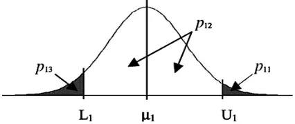
Figure 2. The probabilities of accepted, reworked, and scrapped items (Bowling et al. [4]).
where, P11is the probability of reworking or the
probability of staying in state 1, P12is the probability of
accepting an item, andP13 is the probability of
scrapping an item. Assuming quality characteristics
follow a normal distribution with mean μ1 and standard
deviationσ1.
Thus, these probabilities can be expressed as follows:
21 1 1 2 1
11 1 1
1 1
1 1 .
2
x μ σ
U
P e dx φ U
π σ
(2)
21 1 1
1 2 1
12 1 1 1
1 1
1
. 2
x μ
U σ
L
P e dx φU φ L
π σ
(3)
21 1 1
1 2 1
13 1 1
1
1
. 2
x μ
L σ
P e dx φ L
π σ
(4)
The matrix Pis an absorbing Markov chain where
states 2 and 3 are absorbing and state 1 is transient. As a result, single-stage probability matrix should be rearranged in the following form:
, A O P
Q R
(5)
where, A is identity matrix (2×2), R is a (1×1) matrix
that is included the probability of reworking an item and
Q matrix (1×2) is probability of accepting an item and
the probability of scrapping an item. Thus, by rearranging this matrixs, the following matrix is obtained:
11 12 13
1 0 0
0 1 0 ,
P
P P P
(6)
The fundamental matrix M is obtained as follows [4]:
1 11
11
1
( ) ,
1
M I Q m
p
(7)
where, I is the identity matrix. The long-run absorption
probability matrixF is determined as follows:
1211 1311
,
1 1
P P
F M R
P P
(8)
The elements of the F matrix, f12 and f13 are the
probabilities of an item being accepted and scrapped, respectively. The expected profit per item can be determined using Equation (1), in which it consists of the benefit, processing costs, scrapping cost, and reworking cost per item. The expected benefit is a
selling price per item (SP)multiplied by the probability
of accepting an item (i.e.f12). The expected processing
cost per item isPC1. The expected scrapping cost per
item is the scrapping cost (SC1)multiplied by the
probability of scrapping an item (i.e.f13). When an item
is reworked, the expected reworking cost for a single
visit to the reworking state (i.e., state 1) isRC1. Since
the expected number of times which transient state 1 is
occupied before absorption occurring is m11 - 1thus the
expected rework cost is given by RC m1( 11 - 1).
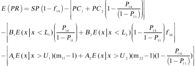
Therefore, the expected profit per item can be expressed as follows:
12 1 1 13 1 11 1 ,
E PR SPf PC SC f RC m (9)
Thus,
13 13 11
1 1 1
11 11 11
1 ,
1 1 1
P P P
E PR SP PC SC RC
P P P
(10)
The equation can be rewritten as follows:
1
1 1
1
1 1
1 1
1
Φ . ( ) Φ
1
Φ Φ( ) Φ
1 Φ . ( )
. 1 Φ( ) Φ
L
1
U
1
L x f x dx L
E PR SP PC B
U L U
U x f x dx A
U U
(11)
The terms Φ L1 and Φ U1 are functions of the decision
In this research, we have assumed that rework cost and scrap cost are not constant and they are function of
mean value of quality characteristics. Thus, RC1and
1
SC can be expressed by an equation as follows:
1 1 1
1 1
1 1
1
f
f ( )
( ) ( )
( ) ,
1 Φ( )
U
U
U
1
RC AE x x U A x x x U dx
x x U xf x dx
A dx A
f x U f x dx
xf x dx A U
(12)
where, A is a constant denoting the coefficient of cost
of reworking an item and E x x
U
is the expectedmean of x when x is larger than U (reworked item).
1 1 1
1 1
1
1 1
f
xf ( ) ( )
,
( ) ( ) Φ( )
L L
L
1
SC BE x x L B x x x L dx
x x L xf x dx xf x dx
B dx B B
f x L f x dx L
(13)
where, Bis a constant denoting the coefficient of cost
of scrapping an item, E x x
L
is expected mean ofx conditioned on being x less than L (scrapped
item).
Constants A and B are parameters of the model that
can be obtained by historical data. If we obtain a regression formula between cost of reworking and value
of quality characteristics then the constant A can be
evaluated. The same method can be applied for
determining the constantB.
Finally, the profit equation is expressed as follows:
1 1 1 1
1 1 1
1 1 1 1
Φ 1
Φ
( )
( ) Φ 1 Φ
,
Φ Φ 1 Φ(U ) Φ
L
U
L
E PR SP PC
U
xf x dx
xf x dx L U
B A
L U U
(14) Thus, 1 1 1 1 1 1 1 Φ 1 Φ ( ) ( ) . Φ Φ L U L
E PR S P P C
U
xf x dx xf x dx
B A U U (15)
The terms Φ
L1 and Φ
U1 are functions of thedecision variable μ1, which is the process mean. We
want to find the value of μ1 that maximizes the
expected profit.
3. 1. Two-stage System Consider a two-stage serial
production system with the following states,
State 1: An item is being processed or reworked in the first stage.
State 2: An item is being processed or reworked in the second stage.
State 3: An item is accepted to be finished items State 4: An item is scrapped
The transition probability matrix is obtained as follows:
11 12 14
22 23 24
0 0
,
0 0 1 0
0 0 0 1
P P P
P P P
P (16)
where, Piiis reworking probability in stage i i ( 1, 2),
1
ii
P is the probability of accepting an item at stage i,
and P14 and P24 is the probability of scrapping an item
at stages 1 and 2, respectively. Thus, the followings are obtained: 12
11 11 22
22
12 23 14 12 24
11 22 11 11 22
23 24
22 22
1
1 1 1
, 1 0
1
1 1 1 1 1
.
1 1
P
P P P
M
P
P P P P P
P P P P P
F P P P P (17)
where, mii1 is the expected number of times that the
transient state i is occupied before absorption
occurring, and f14 is the probability of having a
scrapped item. The expected profit can be determined using Equation (1). We use the objective function proposed by Bowling et al. [4] and revise it to a correct
one. The expected benefit is a selling price per item SP
multiplied by the proportion of accepted items at stage 1
(i.e. 1f14). The expected processing cost is the
expected processing cost per item at stage 1 (i.e., PC1)
plus PC2 multiplied by the probability of accepting an
item at stage 1(i.e.
1411
1 1 P P
. Similarly, the expected
scrapping cost per item is the scrapping cost (SC1)
multiplied by the probability of having a scrapped item at stage 1 (i.e.,
1 1411
P P
) plus SC2 multiplied by the
probability of having a scrapped item at stage 2 (i.e.
14 24 11 (1 ) 1 P f P
). The expected rework cost per item is the
reworking cost (RC1)multiplied by the expected
number of reworking actions for each item at stage 1
(i.e.,m111) plus RC2 multiplied by the expected
number of reworking actions for each item at stage 2
(i.e.m221) multiplied by the probability of accepting
an item at stage 1 that is equal to
1411
Figure 3. A two-stage serial production system (Bowling et al. [4]).
Therefore, the expected profit per item for a two-stage serial production system can be expressed as follows:
14
14 1 2
11
14 14
1 1 2 2 24
11 11
14
1 1 11 2 2 22
11
1 1
1
( ) ( ) 1
1 1
( )(m 1) ( )(m 1)(1 ) , 1
P E PR SP f PC PC
P
P P
B E x x L B E x x L f
P P
P AE x x U A E x x U
P
(18)
where, A1 , A2 are constant numbers that are used for
evaluating RC1 and RC2, respectively and B B1, 2are
constant numbers that are used for evaluating SC1and
2
SC , respectively. Thus, after simplification of the
objective function, following is obtained (Appendix A):
1 1 1 2
1 1 2
1
1 2
1
1 2
1
1 2
1 2
Φ(U ) Φ( )Φ( )
Φ( )
1
Φ( ) Φ( )Φ( )
Φ( )
1 Φ(U )
. ( ) . ( ) Φ(
1
Φ( ) Φ( )
L L
L L
L E PR SP
U U U
L PC PC
x f x dx x f x dx L
B B
U U
1
1 2 1
1 2
1 2 1
)
Φ( )
. ( ) . ( ) Φ( )
1 .
Φ( ) Φ( ) Φ( )
U U
U
x f x dx x f x dx L
A A
U U U
(19)
The terms Φ( )L1 and Φ( )U1 are the functions of the
decision variable μ1 and μ2that are the process means
for stages 1 and 2, respectively.
4. EXTENSION TO MULTIVARIATE NORMAL PROCESS
In this study, quality of items is considered as a model of multivariate data using the multivariate normal distribution.
1 Σ 1
2
1
f , ,Σ
Σ 2
x μ x μ
d
x μ e
π
where, x( , x ii 1,2,..., )d is a vector of
observations that denotes the value of quality
characteristics and μ is 1 by d vector that denotes
the mean value of quality characteristics and Σ is a
d by d symmetric positive definite matrix denoting the covariance among quality characteristics. The multivariate normal distribution is parameterized with a
mean vector, μand a covariance matrixΣ. These are
analogous to the mean μ and variance σ2 parameters
of a uni-variate normal distribution. The diagonal
elements of Σ contain the variances for each variable,
while the off-diagonal elements of Σ contain the
covariance between variables [8]. Assume
( ), 1, 2,..., 2d 1
S m m denotes the mth subset of set
of the variables x ii, 1, 2,...,d (Empty subset is not
considered). If P1 (m)S denotes the probability of
reworking quality characteristics within the subsets
( ), 1, 2,..., 2d 1
S m m among d available
variables then these probabilities can be expressed as follows:
1 Σ 1
2 (m )
1 (m )
1
,
Σ 2
x μ x μ
T
S d
P e dx
π
Ó (20)
where,
, (m)
(m) , .
1,2,...,2 1, 1,2,...,
i i i i i i
d
x U x S
T L x U otherwise
m i d
It is obvious that 2d1 subsets for the set of quality
characteristics
x ii, 1,2,...,d
exist and we shouldevaluate above probability for 2d1 subsets. In
addition, the probability of accepting the items is obtained as follows:
1 Σ 1
2 12
1
,
Σ 2
x μ x μ
T
d
P e dx
π
Ó (21)
where, T Li xi U ii, 1,2,...,d.
The probability of scrapping an item is also obtained as follows:
2 1
13 1 12 1 1 ( ).
d S m m
P P P
(22)
The probabilities of transition among different states of reworked items are also obtained as follows:
1 Σ 1
2 (m )
(m) S(m )
1
,
Σ 2
x μ x μ
T
S d
P e dx
π
Ó
where, (S m) is a subset of set S m( ). Now, we can
1 (1) 1 ( 2 1)
(2 1) S(1) (2 1) (2 1)
1
.
(2 1)
S S d
d
d d d
S S S
P P
Q
S P P
L
M M O M
L
(23)
Furthermore, the probabilities of transition among different states of reworked items and accepted items are obtained as follows:
1 Σ 1
2 ( )
(m)2
1
,
Σ 2
x μ x μ
G m
S d
P e dx
π
Ó (24)
where,
, (m)
G(m) , .
1, 2,..., 2 1, 1, 2,...,
i i i i
i d
L x U x S
x otherwise
m i d
(25)
And probability of scrapping an item is obtained as follows:
2 1
( )3 1 ( ) 2 1 ( ) ( ).
d
S m S m m S m S m
P P P
(26)
Consequently,
12 13
( 2 1) 2 ( 2 1) 3 1
. (2d 1)
d d
S S
P P
R
S P P
M M M (27)
In this research, we have assumed that reworking costs are not constant and they are functions of mean value of
quality characteristics. Thus, RCS m( )can be expressed
by a function as follows:
( ) ( )
(m) ( )
, ( )
,
, ( )
. ,
i i i
S m S m
i
i i i
T S m
i
x U x S m
RC A E x
x Otherwise
x U x S m
A xf x dx
x Otherwise
Ó
(28)
where, AS m( ) is a constant denoting the coefficient of
cost for reworking an item.
Fundamental matrix M is determined as follows:
11 .
M Q
The elements of the F matrix, f12and f13 are the
probabilities of an item being accepted and scrapped that are obtained as follows.
.
F M R (29)
The objective function is also obtained as follows:
12 13
2 1
( ) ( ) (m) 1
( ) ( ) ( )
1 .
d
S m S m S
m
E PR SP f PC SC f
RC m
(30)
4. 1. Discussion about Quality Loss In much conventional industrial engineering, the quality costs are simply represented by the number of items outside specification limits multiplied by the cost of reworking or scrapping. However, Taguchi proposed that manufacturers should consider cost to customers. Loss due to quality has usually only been thought of as additional costs in production to the producer up to the time sale of the product. It was believed that after sale of the item, the consumer was the one to bear quality loss either in repairs or the purchase of a new item. It has been proven in most cases that the manufacturer is the one to bear the costs of quality loss due to things like negative feedback from customers. Though the initial costs are those of non-conforming items, any item manufactured away from mean value would lead to some loss to the customer. These losses are major costs and are usually ignored by designers, which are more interested in their private costs than social costs. Such terms prevent suppliers from operating efficiently, according to social economics. Such losses would inevitably find their way back to the production environments and suppliers and it would reduce income [8]. Reworking and scrapping costs are samples of private costs for manufacturer. Manufacturer is the one to bear these costs directly. However, cost of quality loss that is modeled by Taguchi loss functions is a sample of social cost. The manufacturer is the one to bear this cost indirectly. Even though both type of cost are a function of optimal process mean but they are actually different type of costs that have different source of variation. Cost of quality loss is usually ignored in such problems. This cost is usually evaluated based on Taguchi loss function [9]. Taguchi loss function for this problem is obtained as follows:
Taguchi loss function=
2
1
1 Σ 1
2 2
1
1 Σ 1 2
( )
, 1, 2, ..., 1
( )
Σ 2
, 1
,
Σ 2
d
i i
i
i i i
x μ x μ
d
Ti i i d
x μ x μ
T
d
R x μ
E
T L x U i d
R x μ e dx
π
e dx
π
Ó
Ó
(31)
where, R is constant parameter that is determined by
historical data. Now, the expected profit per item is obtained as follows:
12 13
2 1
( ) ( ) ( ) 1
( ) ( ) ( )
(m 1) Taguchi Loss Function
d
S m S m S m
m
E PR SP f PC SC f
RC
(32)
4. 2. Applications to Bi-variate Normal Case
Assume that two quality characteristics ,x y follow a
bi-variate normal distribution as follows:
( )
( )2 2 2
1
2 2 1
2
1 ,
2 1
y y
x x
x y x y
y y
x x
x y
f x y e
m m
m r m
s s s s
r
ps s r
ææ - ö æ - ö æ - öæ - öö
ç ç ÷ ç ÷÷
- çç ÷+ç ÷- ç ÷ç ÷÷
ç ÷
- èè ø è ø è øè øø =
-(33)
Assuming that quality characteristics are independent, following equations are obtained,
( )
( )
2
2
1 2
1 2
1
, 2
1
. 2
x x
y y
x
x
y
y
f x e
f y e
m s
m s
s p
s p
ææ - ö ö
ç ÷
- çç ÷ ÷
è ø
è ø
ææ - ö ö çç ÷ ÷ - çççè ÷ø ÷÷
è ø
=
=
The notations USLx, LSLx are the upper and lower
specification limits for the characteristic x and the
notations U S Ly, L SLy are the upper and lower
specification limits for characteristicy. In a process, if a
quality characteristic was less than its lower specification limit then the item is considered as scrapped, and if it was more than the upper specification limit then the item needs to be reworked. Other notations are defined as:
:
x
c The coefficient of cost of reworking characteristic
x
:
y
c The coefficient of cost of reworking characteristic
y
:
xy
c The coefficient of cost of reworking characteristic
, x y
:
c Cost of a scrapped item
:
pc Processing cost for each item
:
SP The profit per item
For a single-stage production system with the following states:
State 1: An item is being processed by the production system
State 2: The characteristic x is being reworked.
State 3: The characteristic yis being reworked.
State 4: The characteristics ,x y are being reworked.
State 5: An item is accepted to be finished item. State 6: An item is scrapped.
The single-step transition probability matrix can be expressed as:
1 2 3 4 5 6 1
12 13 14 15 16 2
22 25 26
3
33 35 36 4
42 43 44 45 46
5
6
0
0 0 0
0 0 0
0
0 0 0 0 1 0
0 0 0 0 0 1
P P P P P
P P P
P P P
P P P P P
P=
é ù
ê ú
ê ú
ê ú
ê ú
ê ú
ê ú
ê ú
ë û
(34)
where,
12
P : The probability of reworking the characteristics x
13
P : The probability of reworking characteristics y
14
P : The probability of reworking both characteristics
, x y
15
P : The probability of accepting an item
16
P : The probability of a scrapping an item
Moreover, for the characteristicx, P25 denotes the
probability of accepting an item andP26, denotes the
probability of scrapping an item after reworking
characteristicx. For characteristic y, those are P35and
36
P .
Finally, P45and P46 denote the probabilities of accepting
and scrapping an item after reworking characteristic x
and y.
Assuming that the quality characteristics of an item follow a bi-variate normal distribution, therefore the probabilities can be expressed as follows:
{
}
(
)
( )
12 42 Pr ,
,
( )
y y x
y
y x
x y y
USL
LSL USL
USL
LSL USL
p p x USL LSL y USL
f x y dxdy
f y f x dx
¥
¥
= = > £ £ =
=
ò ò
ò
ò
{ } ( )
{ } ( )
{ } ( )
22
25
26 Pr
Pr
Pr
x x x x
x USL
USL
x x LSL
LSL x
p x U SL f x dx
p LSL x U SL f x dx
p x LSL f x dx
¥
-¥ = > =
= < < =
= < =
ò
ò
ò
{
}
( )
( )
13 43 Pr ,
,
( )
x
x y
x
x y
y x x
USL
LSL USL
USL
LSL USL
p p y USL LSL x USL
f x y dydx
f x f y dy
¥
¥
= = > £ £
=
ò ò
=ò
ò
{
}
( ){
}
( ){
}
( )33
35
36
Pr
Pr
Pr
y y
y y
y USL
USL
y y
LSL LSL y
p y USL f y dy
p LSL y USL f y dy
p y LSL f y dy
¥
-¥
= > =
= < < =
= < =
ò
ò
ò
{
}
(
)
( )
14 44 Pr ,
, ( ) y x y x x y USL USL USL USL
p p x USL y USL
f x y dxdy
f y f x dx
¥ ¥
¥ ¥
= = > >
=
ò ò
=ò
ò
{
}
(
)
( )
15 45 Pr ,
, ( ) y x y x y x y x
x x y y
USL USL
LSL LSL USL USL
LSL LSL
p p LSL x USL LSL y USL
f x y dxdy
f y f x dx
= = £ £ £ £
=
ò ò
=ò
ò
{
}
(
)
(
)
(
)
16 46 Pr or
, , , ( ) ( ) ( ) ( ) y x y x y x y x x y LSL LSL LSL LSL LSL LSL LSL LSL
p p LSL x LSL y
f x y dxdy f x y dydx
f x y dxdy
f y dy f x dx
f y dy f x dx
¥ ¥
-¥ -¥ -¥ -¥
-¥ -¥
-¥ -¥
-¥ -¥
= = > > =
+
- =
+
-ò -ò
ò ò
ò ò
ò
ò
ò
ò
To analyze the absorbing Markov chain, the transition
matrix P is rearranged to the following matrix:
I . P éê ùú
ë û
O =
R Q (36)
Therefore,
5 6 1 2 3 4 5
6
1 15 16 12 13 14
2
25 26 22
3 35 36 33
4
45 46 42 43 44
1 0 0 0 0 0
0 1 0 0 0 0
0
0 0 0
0 0 0
0
P P P P P
P
P P P
P P P
P P P P P
= é ù ê ú ê ú ê ú ê ú ê ú ê ú ê ú ê ú ë û (37)
Fundamental matrix M is determined as follows:
( )
( )
( )( ) (( )() ) ( )
( )( ) ( )( )
1
12 13 14
-1 22
33
42 43 44
12 44 14 43 12 44 42 14 14
22 44 33 44 44
22
33 43 42
22 44 33 44 44
1
0 1 0 0
-0 0 1 0
0 1
1 1
1
1 1 1 1 1
1
0 0 0
1
1
0 0 0
1
1 0
1 1 1 1 1
P P P
P M I Q
P
P P P
P P P P P P P P P
P P P P P
P
P P P
P P P P P
-- -
-é ù
ê - ú
ê ú
= = =
ê - ú
ê - - - ú
ë û
é - + - + ù
ê - - - - - ú
ê ú ê ú ê ú -ê ú ê ú ê ú -ê ú ê ú ê - - - - -êë û . ú ú (38)
The absorption probability matrix F is determined as
follows (Bowling et al. [4]):
F M R
where, f15 and f16are the probabilities of accepting and
scrapping one item respectively that are obtained as follows:
12 44 14 43 15 15 25
22 44
12 44 42 14 14
35 45
33 44 44
(1 )
1 1
(1 )
,
1 1 1
P P P P
f P P
P P
P P P P P
P P
P P P
(40)
16 1 15.
f f (41)
Now, the expected profit per item can be defined as:
( )
1522
33
44
16
( 1) ( )
( 1) ( )
( 1) ( ) ( )
x y xy x y x y
E PR f SP pc
m E x x USL c
m E y y USL c
m E x x USL E y y USL c
f c
= -
-- >
-- >
-- > >
-( )
( )
( ) x
x USL x
USL
xf x dx E x x USL
f x dx
¥
¥
> =
ò
ò
( )
( )
( ) y
y USL y
USL
yf y dy E y y USL
f y dy
¥
¥
> =
ò
ò
(42)
with substituting, f15 and f16, the optimal values of μx
and μythat maximize the expected profit can be
reached.
5. NUMERICAL EXAMPLES
5. 1. Single-stage System The above model can be
illustrated by a numerical example. Consider a
single-stage production system with parameters:
1
120, 25,
SP PC A110, B115,
1 1, 1 8 , 1 12
σ L U .
Parameters are taken from Bowling et al. [4]. It is seen
that the expected profit is maximized at μ110.1 and
the profit per item is 87.024. Figure 1 shows the expected profit as a function of the process mean. As it can be seen, the expected profit is concave over the interval[L1 8,U112].
5. 2. Two-Stage System Consider a two-stage
production system with following parameters:
1 2 1 2
1 2 1 2 1
2 1 2
120, 25, 20, 10, 17,
15, 12, 1, 8,
13, 12 , 17.
SP PC PC A A
B B σ σ L
L U U
Parameters are taken from Bowling et al. [4]. It is seen
that the expected profit is maximized at μ110.1 and
1 15.2
Figure 2 shows the expected profit as a function of the
process means (μ μ1, 2). It is seen that the expected
profit is concave in the specified intervals,
1 1 2 2
[L 8,U 12],[L 13,U 17].
Figure 4. Expected profit versus process mean
Figure 5. Effect of changing process means on the expected process.
Figure 6. Effect of changing process means on the expected profit per item in bivariate process.
Table 1 denotes the results for one stage and two- stage model. As can be seen the optimal adjustment is a little more than the half point of specification limits that is because of the less values of reworking cost in comparison with scrapping cost.
5. 3. Bi-variate Normal Process Consider a
single-stage production system with the following parameters:
120, 45, 1, 0.5, 20, 1, 0 , 8.0, 13.0,
12.0, 17.0, 0.1.
x y x y
x y
x y xy
SP pc c c c σ σ
ρ L L
U U c
According to Fallahnezhad and Hosseini nasab [7], a similar model is solved with assuming the condition that reworking action can be performed one time on each item when dual quality characteristics existed. It is seen
that the expected profit is maximized at μx10.15
and μy= 14.8, the profit per item is 64.795. Figure 6
shows the expected profit as a concave function of the process means. Since the reworking cost of quality
characteristics y may be more than scrapping cost, it is
seen that the mean of quality characteristics y is
optimized below the half point of specification interval.
TABLE 1. Expected profit and optimal mean values
One Stage Two Stages Bi-variate
1 or x
μ μ 10.1 10.1 10.15
2 or y
μ μ - 15.2 14.95
( )
E PR 87.024 54.438 64.795
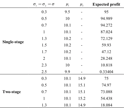
TABLE 2. Sensitivity analysis for a single and two-stage production system
1 2
σ σ σ μ1 μ2 Expected profit
Single-stage
0.3 9.5 - 95
0.5 10 - 94.989
0.7 10.1 - 94.272
1 10.1 - 87.024
1.3 10.2 - 72.129
1.5 10.2 - 59.93
1.7 10.2 - 47.12
2 10.1 - 28.248
2.3 10 - 10.818
2.5 9.9 - 0.33404
Two-stage
0.3 10.1 14.9 75
0.5 10.1 15.1 74.97
0.7 10.1 15.1 73.088
1 10.1 15.2 54.438
6. SENSITIVITY ANALYSIS
Table 2 shows the variations of the optimum process mean and the optimum expected profit with changing the standard deviation parameter in single and two-stage production systems. As can be seen, with increasing
parameter σ , first the optimal mean increases and then
decreases. This shows that the optimal mean is a
concave function of the parameterσ . In addition, it is
seen that with increasing parameter σ , the expected
profit decreases that is reasonable because with
increasing the value of parameterσ, the probabilities of
scrapping and reworking increases that leads to decrease the expected profit. It is also seen that when standard deviation sufficiently increases then the value of optimal process mean will be less than the half point of specification limits. With increasing standard deviation, the probability of reworking an item increases. Thus, the expected number of times that the reworking state is occupied increases too. Therefore, the total cost of reworking an item may be more than cost of scrapping an item (considering the number of reworking actions is performed on item). Moreover, the optimal process mean will be adjusted below the half point of specification limits.
7. DISCUSSION AND CONCLUSIONS
In this research, the objective was to determine the optimum process target levels for a serial production system. The main contribution of the paper is to consider the variable costs as a function of decision variable that its application is justified based on using a conditional mean equation. The model can be applied in the cases that scrapping and reworking costs are not constant for different items and the value of quality characteristics can influence on these costs. It is shown that the objective function is concave. Therefore, the maximization of the profit is possible over the specified limits. Another contribution of this model is to extend proposed model to multivariate normal process. Numerical examples and sensitivity analysis show the application of the proposed method. As future research, we propose to consider the problem of Multi-stage production system when several quality characteristics existed in each stage. In addition, analyzing the effects of variation of covariance matrix in multi-variate normal distribution is suggested as future research.
8. ACKNOWLEDGMENT
The authors are deeply thankful to the reviewers and the editor for their valuable suggestions to improve the manuscript.
9. REFERENCES
1. Fallahnezhad, M., Niaki, S. and Zad, M. V., "A new acceptance sampling design using Bayesian modeling and backwards induction", International Journal of Engineering-Transactions C: Aspects, Vol. 25, No. 1, (2012), 45.
2. Rahim, M. and Al-Sultan, K. S., "Joint determination of the optimum target mean and variance of a process", Journal of Quality in Maintenance Engineering, Vol. 6, No. 3, (2000), 192-199.
3. Tosirisuk, P., "Economic design of process parameter control limits and process adjustment intervals for continuous production processes", Computers & Industrial Engineering, Vol. 19, No. 1, (1990), 263-266.
4. Bowling, S. R., Khasawneh, M. T., Kaewkuekool, S. and Cho, B. R., "A Markovian approach to determining optimum process target levels for a multi-stage serial production system",
European Journal of Operational Research, Vol. 159, No. 3, (2004), 636-650.
5. Khasawneh, M. T., Bowling, S. R. and Cho, B. R., "A Markovian approach to determining process means with dual quality characteristics", Journal of Systems Science and Systems Engineering, Vol. 17, No. 1, (2008), 66-85.
6. Nezhad, M. S. F. and Niaki, S. T. A., "Absorbing Markov Chain Models to Determine Optimum Process Target Levels in Production Systems with Rework and Scrapping", Journal of Industrial Engineering, Vol. 6, No., (2010), 1-6.
7. Fallah Nezhad, M. S. and Hosseini Nasab, H., "Absorbing Markov Chain Models to Determine Optimum Process Target Levels in Production Systems with Dual Correlated Quality Characteristics", Pakistan Journal of Statistics and Operation Research, Vol. 8, No. 2, (2012).
8. Abbasi, B., Niaki, S. T. A. and Arkat, J., "Optimum Target Value for Multivariate Processes with Unequal Non-Conforming Costs", Journal of Industrial Engineering International, Vol. 2, No. 3, (2006), 1-12.
9. Fallahnezhad, M. and Fakhrzad, M., "Determining an Economically Optimal(N, C) Design via Using Loss Functions",
International Journal of Engineering, Vol. 25, No. 3, (2012), 197-201.
APPENDIX
Obtaining the expected profit per item for two-stage serial production system
The expected profit per item for a two-stage serial production system can be expressed as follows:
14
14 1 2
11
14 14
1 1 2 2 24
11 11
14
1 1 11 2 2 22
11
1 1
1
( ) ( ) 1
1 1
( )(m 1) ( )(m 1)(1 ) ,
1 P
E PR SP f PC PC
P
P P
B E x x L B E x x L f
P P
P
A E x x U A E x x U
P
where, A1 , A2 are constant numbers that are used for
evaluating RC1 and RC2 ,respectively and B1 , B2 are
constant numbers and are used for evaluating SC1 and
SC2 ,respectively .Thus we have,
14 12 24 14
1 2
11 11 22 11
1 2
14
1 2
1 11 1
1
1 1 1 1
. ( ) . ( )
Φ(L ) 1 Φ( )
L L
P P P P
SP PC PC
P P P P
x f x dx P x f x dx
SC SC
P L
14 24
11 22
1 11 2 12 14
1 2
1 11 2 22 11
1
1 1
. ( ) . ( )
1 .
1 Φ( ) 1 1 Φ( ) 1 1
U U
P P
P P
x f x dx P x f x dx P P
RC RC
U P U P P
Equivalently we have,
1 1 2
1 1
1 2
1 1 2 1
1 2
1
1 2
1 1 2
Φ(U ) Φ( )Φ( )
Φ( ) Φ( )
1 1
Φ( ) Φ( )Φ( ) Φ(U )
. ( ) Φ . ( )
Φ( ) Φ Φ(L )
L L
L L
L L
E PR SP PC PC
U U U
x f x dx L x f x dx
B B
U U
1 2
1 2
1 1 2 2 1
1 2
1 1 2 2
Φ( ) Φ( )
1
Φ( ) Φ( )
. ( ) 1 Φ( ) . ( ) 1 Φ( ) Φ( ) 1 1 Φ( ) Φ( ) 1 Φ( ) Φ( ) Φ(
U U
L L
U U
x f x dx U x f x dx U L
A A
U U U U
1
. )
U
Therefore following is concluded,
1 1 1 2 1
1 2
1 1 2 1
1 2
1 2
1 2
Φ(U ) Φ( )Φ( )
Φ( ) Φ( )
1 1
Φ( ) Φ( )Φ( ) Φ(U )
. ( ) . ( ) Φ
1
Φ( ) Φ( )
L L
L L
L L
E PR SP PC PC
U U U
x f x dx x f x dx
B B
U U
1 1 2 1
1 2
1 1 2 1
. ( ) . ( )
( ) Φ( )
1 .
Φ( ) Φ( ) Φ( ) Φ( )
Ux f x dx U x f x dx
L L
A A
U U U U
Optimal Process Adjustment with Considering Variable Costs for
Uni-variate and Multi-variate Production Process
RESEARCH NOTE
M. S. Fallahnezhad, E. Ahmadi
Department of Industrial Engineering, Yazd University, Yazd, Iran
P A P E R I N F O
Paper history:
Received 25 December 2013
Received in revised form 07 August 2013 Accepted 22 August 2013
Keywords:
Markov Chain Process Mean Normal Distribution
هﺪﯿﮑﭼ
رد ﻪﻟﺎﻘﻣﻦﯾا ، ﻢﺘﺴﯿﺳ يﺎﻫ ﺪﯿﻟﻮﺗ ي
ياﻪﻠﺣﺮﻣودوياﻪﻠﺣﺮﻣﮏﺗ
ﻦﺘﻓﺮﮔﺮﻈﻧردﺎﺑ
ﯽﺳرزﺎﺑياﺮﺑﯽﺴﻧاﺮﻠﺗيﺎﻫﺖﯾدوﺪﺤﻣ
، درﻮﻣ
ﻪﻌﻟﺎﻄﻣ راﺮﻗ
ﺖﺳاﻪﺘﻓﺮﮔ
.
ﯽﻔﯿﮐﻪﺼﺨﺸﻣراﺪﻘﻣﻪﮐﯽﻣﺎﮕﻨﻫ
ﺎﭘ ﯿﯾ ﻦ ﺮﺗ زا
ﯽﻨﻓﻪﺼﺨﺸﻣﺪﺣزاﺮﺗﻻﺎﺑﺎﯾوﻦﯿﯾﺎﭘﯽﻨﻓﻪﺼﺨﺸﻣﺪﺣ
ﻻﺎﺑ
ﺪﺷﺎﺑ ، ﻪﻌﻄﻗ ﯾﺎ ﻞﯾﺪﺒﺗ دراديرﺎﮐهرﺎﺑودﻪﺑزﺎﯿﻧﺎﯾودﻮﺷﯽﻣتﺎﻌﯾﺎﺿﻪﺑ
.
ﻦﯿﯿﻌﺗ،فﺪﻫ
ﺢﻄﺳ ﻦﯿﮕﻧﺎﯿﻣ ﻬﺑ ﯿ ﻪﻨ ﺮﺑﺪﻨﯾاﺮﻓﮏﯾياﺮﺑ
ويرﺎﮐهرﺎﺑوديﺎﻫﻪﻨﯾﺰﻫسﺎﺳا
ﻪﻨﯾﺰﻫ
ﺖﺳاتﺎﻌﯾﺎﺿ
.
،ﯽﻠﺒﻗتﺎﻌﻟﺎﻄﻣفﻼﺧﺮﺑ
ﻮﺷﯽﻤﻧﻪﺘﻓﺮﮔﺮﻈﻧردﺖﺑﺎﺛﺎﻫﻪﻨﯾﺰﻫ
ﺪﻧ
.
ردﻦﯿﻨﭽﻤﻫ
ﻪﻟﺎﻘﻣﻦﯾا ،
ياﺮﺑﯽﻓﻮﮐرﺎﻣلﺪﻣﮏﯾ ﺖﺳاهﺪﺷهدادﻪﻌﺳﻮﺗهﺮﯿﻐﺘﻣﺪﻨﭼلﺎﻣﺮﻧيﺎﻫﺪﻨﯾاﺮﻓ
.
لﺎﺜﻣ يﺎﻫ
نﺎﺸﻧياﺮﺑيدﺪﻋ
ﺖﺳاهﺪﺷمﺎﺠﻧاهﺪﺷﻪﺋاراشوردﺮﺑرﺎﮐنداد
.
![Figure 3. A two-stage serial production system (Bowling et al. [4]).](https://thumb-us.123doks.com/thumbv2/123dok_us/233314.2017942/5.595.59.241.439.568/figure-stage-serial-production-bowling-et-al.webp)