Image Denoising Using Anisotropic Diffusion Equations on Reflection and illumination Components of Image

Please cite this article as: M. H. Khosravi and H. Hassanpour, Image Denoising Using Anisotropic Diffusion Equations on Reflection and illumination Components of Image, International Journal of Engineering (IJE), TRANSACTIONS C: Aspects Vol. 27, No. 9, (September 2014) 1339-1348,

International Journal of Engineering

J o u r n a l H o m e p a g e : w w w . i j e . i r

Image Denoising Using Anisotropic Diffusion Equations on Reflection and

Illumination Components of Image

M. H. Khosravi*, H. Hassanpour

Department of Computer Engineering, University of Shahrood, Shahrood, Iran

P A P E R I N F O

Paper history:

Received 06 January 2014

Received in revised form 13 April 2014 Accepted 22 May 2014

Keywords: Image Denoising Image Smoothing Anisotropic Diffusion Homomorphic Filtering Hybrid Image Enhancement

A B S T R A C T

This paper proposes a new hybrid method based on Homomorphic filtering and anisotropic diffusion equations for image denoising. In this method, the Homomorphic filtering extracts the reflection and illumination components of a noisy image. Then a suitable image denoising method based on anisotropic diffusion is applied to each components with its special user-defined parameter. This hybrid scheme donates a flexibility and customizability to the method, due to its ability in properly enhancing images components. In order to evaluate the proposed method effectiveness, a number of experiments have been performed and the results have been compared with the results of other pioneering methods. The good results indicate superiority of the proposed method.

doi: 10.5829/idosi.ije.2014.27.09c.03

1. INTRODUCTION1

Image denoising is an active research scope in the context of image processing and analysis. A dozen of methods are suggested to vanish variety of noises from images and to generate clean and information rich version of them. Some of them have simple ideas and use simple filters, such as average filters and Gaussian filters [1]. However, these simple linear methods, which have been very popular for their simplicity and speed, tend to blur image. With the aim of solving this unwanted effect, some nonlinear methods have been proposed and implemented, such as median filter, Perona-Malik anisotropic diffusion [2, 3], the Rudin– Osher–Fatemi total variation model [4], Yaroslavsky neighborhood filters [5], SUSAN filter [6], Wiener local empirical filter [7], the wavelet thresholding [8], DUDE and the discrete universal denoiser [9] and some fuzzy based methods available in the literature [10]. These methods are more time consuming than linear approaches, but they perform much better in general.

1_{*Corresponding Author’s Email: [email protected]} (M. H. Khosravi)

Here we will focus mainly on anisotropic diffusion method, which also called Perona-Malik diffusion. This method is an extension to isotropic diffusion which is a blurring process motivated from scale space concept. The isotropic diffusion like Gaussian blurring filter is a space-invariant transformation and removes edges, lines or other details of image contents during smoothing. In contrast, the anisotropic diffusion is a space-variant and non-linear transformation of original image, which behaves localy at different image regions. In regions close to the edges, this method diffuses along the edges, but not across them. Unlikely, in smooth areas the method performs standard isotropic diffusion. This flexibility is obtained using an anisotropic diffusion factor, also called edge-stoping factor, which controls the smoothing process in regions that have edges. After Perona-Malik model, many modifications to anisotropic diffusion model have been proposed. Alvarez et al. [11] considered the direction information of edges and proposed a mean curvature motion (MCM) anisotropic diffusion. In their proposed method, the diffusion only applied in a direction parellel to edges, but not across edges. Catte et al. [12-14] found that diffusion process in very similar images could output divergent solutions. In their proposed solution, the image gradient is

obtained from smoothed version of image. Weickert [15] proposed a coherence-enhancing diffusion (CED) model which preserves the coherence structures of edges. In 2002, Gilboa [16] proposed a forward and backward adaptive diffusion which could sharpen the edges in backward process, in addition to smoothing noises in forward proecss. In addition to these theoretic improvements, some heuristic approachs, also, tried to improve the results of anisotropic diffusion. In some works [17] the diffusion process was applied on neighbors longer than one pixel. To better preserve edges in this technique, slant edges are considered in addition to vertical and horizontal edges. In another work [18] a method based on anisotropic diffusion and wavelet transform was proposed. In their proposed method, anisotropic diffusion is applied on the approximation band in the wavelet domain. Similarly, the authors in another research [19] worked on PDE-based noise reduction technique but using a fourth order PDE. Here we intend to use another combinatorial scheme in which the results of traditional anisotropic diffusion will be improved. In spite of preserving the strong edges, some weak edges or non-edge details may be blurred and be vanished via applying traditional anisotropic diffusion method. In this study, we improve denoising process to preserve more details in image. In our suggestion, the noisy image first is splitted into two major components, reflection and illumination, via a Homomorphic filtering. To achieve more smoothed image with better-preserved edges, the anisotropic diffusion is performed on these components, separately. The major motivation of this suggestion was the paper available in the literature [20], which emphasizes the power of applying image enhancement method on each image components, reflection and illumination, separately. Edges, even weak edges, in noisy image will be strong one in reflection component, and so the diffusion process will smooth them less. On the other hand, the illumination component has less edge information and can be smoothed in less iterations. Finally, noiseless image will be achieved by joining the weighted versions of these two processed components.

The rest of the paper is organized as follows: the concepts of Homomorphic filtering and anisotropic diffusion are illustrated in Sections 2 and 3. Proposed method is introduced in Section 4. Section 5 and its subsections describe some evaluation metrics, which will be used at the consequent sections. Experimental results of proposed method and discussion around it are the last sections.

2. HOMOMORPHIC FILTERING

The illumination-reflectance model is one of the most attractive models of an image, which describes the gray

level image function I(x,y) as two components, reflection, 0<r(x,y)<1 and illumination, 0<i(x,y)<¥ as

below:

) , ( ). , ( ) ,

(x y i xy r xy

I = (1)

The reflection component is an approximate model of the object, while the illumination component illustrates the environment lightening and is determined by illumination sources [21]. The image quality can be improved by extracting these two components by a procedure called homomorphic filtering [21] and enhancing each of them in an appropriate manner [20]. To extract these components via Homomorphic filtering, the Fourier transform is used. However, since the Fourier transform of the product of two function is not separable, the natural logarithm of the image is taken as follows:

) , ( ln ) , ( ln ) , (

lnI x y = ix y + r x y ₍₂₎

Then the Fourier transform is applied to this function:

)} , ( {ln )} , ( {ln )} , (

{lnI x y =Á ix y +Á r x y

Á ₍₃₎

where Á{.} denotes the Fourier transform. This form of

image representation allows us to separate the illumination and reflectance components and then apply desired filters. We can approximately describe the illumination component of an image as its low frequency component in the frequency domain, since its representation in the spatial domain is characterized by slow and uniform variations. In contrast, the reflectance corresponds to the high frequency component in the frequency-domain, due to its rapid gray level variations in spatial domain. Therefore, these two components can be separated by applying two appropriate high pass and low pass filters. Now each of these components can be accessed to enhance the overall image or act as a preprocessing stage in an outer procedure.

3. ANISOTROPIC DIFFUSION

State space modelling is a good framework to represent a signal in a multi-scale view. For an image function

) , (xy

I _{, state space representation is a family of signals}

) ; , (x yt

I _{, which defined as} I(x,y;t)=G(x,y;t)*I0(x,y), where

‘*’ stands for convolution operator, I(x,y;0)=I0(x,y)

and G(x,y;t) _{is a Gaussian kernel:}

t y x

e t t y x

G (2 2)/2

2 1 ) ; ,

( = - +

p (4)

The scale parameter t in above definitions indicates the scale level. Koenderink [22] and Hummel and Moniot [23] showed that the state space family of images can be defined as the solution of the diffusion Equation (5), as below:

) , , ( ) , ,

( 2

t y x I t

t y x

I _{= Ñ}

¶

¶ _a

Diffusion is a physical process that can be modeled as a Gaussian smoothing process whose variance increases continuously. By applying this form of diffusion, which is called isotropic diffusion, the image regions become smooth, but, as a bad side effect, the edges of the regions become blurred, because of the globally smoothing. Perona and Malik [3] proposed anisotropic diffusion in which the smoothing process may be performed differently in each direction, as follows:

)) , , ( ) , , ( ( ( ) , , (

t y x I t y x I c div t

t y x

I _{= Ñ Ñ}

¶

¶

(6)

where Ñ is the gradient operator, div stands for divergence operator, ÑI is the magnitude of ÑI and c(.) is the diffusion (or conductance) function which controls the rate of diffusion. If the diffusion factor c(.) has a constant value, then it is called isotropic diffusion factor. In this case, there is no difference between pixels in different regions and all of them are smoothed uniformly. To avoid this undesired deficiency, the diffusion factor c(.) must be a function of x and y at the moment of t. Two choices for such an anisotropic diffusion factor was suggested by Perona and Malik [3] as below:

) exp( )

( ₂

2

k I I

c Ñ = - Ñ (7)

) 1 (

1 ) (

2 2

k I I

c

Ñ + = Ñ

(8)

The value of k in Equations (7) and (8) is used to control the diffusion factor and is determined by user. The Perona and Malik anisotropic diffusion scheme is incapable of efficiently denoising images suffering a high level of noise. Indeed the gradient operator is susceptible to noise and so it is not a reliable measure to face with strong noises [12-14]. Catte suggests that the diffusion function must be applied on the smoothed version of image [12-14]. Therefore, the parameter of diffusion function will be ÑG_s*I instead of ÑI where Gsis a Gaussian smoothing kernel and ‘*’ is the convolution operator. So the Equation (5) becomes as below:

)) , , ( ) , , ( * ( ( ) , , (

t y x I t y x I G c div t

t y x

I _{= Ñ Ñ}

¶ ¶

s (9)

In this paper, we will compare the results of our proposed method with these two original schemes.

4. PROPOSED METHOD

Recently, many efforts have been done to develop a hybrid algorithm for image enhancement in which adopted anisotropic diffusion is a part of their suggested system [24-26]. In a hybrid system one subsystem can play the role of a preprocessing stage to deliver a better

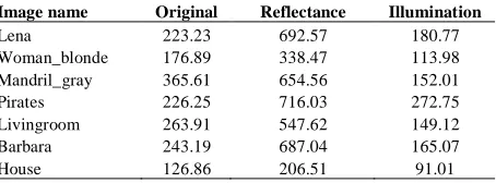
input to the second subsystem, or can act like a postprocessing one to enhance the output of the other process. Our proposed idea, is based on the work available in the literature [20], which emphasizes on the power of applying a proper enhancement method on each of the two image components, reflectance and illumination. We know that diffusion function in Perona and Malik scheme is sensitive to edges and will report lower values where the strength of the edge is higher. But weak edges may be blurred and be vanished by this scheme. Our proposed method can be considered as a preprocessing stage trying to improve the image contrast via extracting its reflectance and illumination components using a Homomorphic filter. Our observations show that the reflection components have better contrast compared to the original image and hence expected to have more efficient and strong edges than original image. To quantify this observations, we evaluate the contrast of an image by computing the mean of the local variance map (MLV). This map is formed by substituting each pixel with the local variance of a 3×3 neighborhood pixel values. The mean value of the overall map is a good metric for assessing the contrast of the corresponding image. This metric has a low value (close to zero) for a low contrast image and a high value for a high contrast one. For an image with uniform distribution this metric is equal to 0. In Figure 1, the Lena image and its reflectance and illumination components are shown. In addition, Table 1, illustrates the MLV values for some standard test images, which emphasizes that reflectance component of each image has more contrast than the original image.

(a) (b) (c)

Figure 1. (a) Original image of Lena (with MLV=223.23), (b) its reflectance (with MLV=692.57) and (c) illumination (with MLV = 180.77).

TABLE 1. Mean of the Local Variance (MLV) for some standard images and their reflectance and illumination components

Image name Original Reflectance Illumination

Lena 223.23 692.57 180.77

Woman_blonde 176.89 338.47 113.98

Mandril_gray 365.61 654.56 152.01

Pirates 226.25 716.03 272.75

Livingroom 263.91 547.62 149.12

Barbara 243.19 687.04 165.07

Figure 2 shows an enlarged version of Lena image (Figure 1), and illustrates that reflectance component has more details and stronger edges than the original image. This property helps the anisotropic diffusion to smooth this details less.

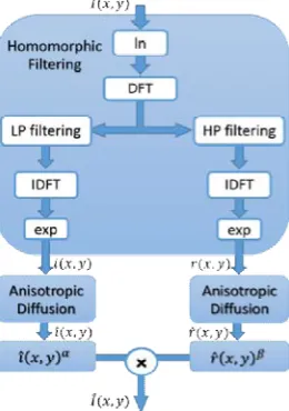
After splitting the noisy image into reflection and illumination components, we apply the proper anisotropic diffusion on each component. Finally with aggregating these two processed components, our denoised image is achieved. This process is illustrated in Figure 3. In anisotropic diffustion process, to discretize the diffusion Equation (6) we used the Perona and Malik scheme as below:

å

+ _{= + Ñ Ñ}

j i

d d d

j i t

j i t

j

i I c I I

I

,

) ( ,

, 1

, _h

h l

(10)

where t j i

I, is our image intensity at point (i,j) in iteration

step t and c(.) is diffusion function. The constant value

[ ]

l determines the diffusion rate and hi,jdenotes

the spatial 4-pixel neighborhood of pixel

} , , , { : ) ,

(i j hi,j= NSEW, where N, S, E and W stands for the North, South, East and West neighbors, respectively. Obviously the scalar h_i,_j is equal to 4 in this context.

(a) (b)

Figure 2. Cropped and zoomed version of images in Figure 1; (a) original image of Lena and (b) reflectance component.

Figure 3. Proposed hybrid scheme to image denoising.

Figure 4. Four directions to calculate Ñd.

In discretized form, the symbol Ñd denotes the difference between neighboring pixels in directions d as follow (see Figure 4):

j i j i NI=I 1, -I,

Ñ - , ÑSI=Ii+1,j-Ii,j

j i j i EI =I, 1-I,

Ñ + , ÑWI=Ii,j-1-Ii,j

(11)

The diffusion Equation (10) can be summarized as:

(

)

ú ú û ù ê

ê ë é

Ñ Ñ +

=

å

Î +

I I c I

I d

E W S N d

d t

j i t

j i

} , , , { , 1

, l (12)

5. PERFORMANCE MEASURES

To evaluate our results and having some comparative mechanism to assess our proposed method, we use some metrics that are described briefly in below subsections.

5. 1. Mean Square Error (MSE) Perhaps the

simplest and oldest objective image quality measure is the MSE [27], which denotes the overall difference between noisy and original images. For two images X and Y with dimenstions m×n, the MSE is defined as below:

( ) ( )

(

)

åå

-=

-= 1

0 1

0

2 , , 1 m

i n

j

j i Y j i X mn

MSE (13)

5. 2. Peak Signal to Noise Ratio (PSNR) The

PSNR that is a common metric to compare two images indicates the ratio between the maximum possible powers of two images. This metric use the MSE in its formula as below [27]:

MSE L PSNR

2 10

log 10

= (14)

where L is the maximum possible pixel value of the image. For gray scale images, L=28-1=255.

5. 3. Structural Similarity Index Measure (SSIM)

two images x and y with the following expression [28],

( ) ( )

[

] ( )

[

] ( )

[

]

y x s y x c y x l y x

S , = , . , . , (15)

which is constructed by three similarity components: illumination similarity, l(x,y) contrast similarity, c(x,y)

and structural similarity, s(x,y) as defined below:

1 2 2 1 2 ) , ( C C y x l y x y x + + + = m m m m (16) 2 2 2 2 2 ) , ( C C y x c y x y x + + + = s s s s ₍₁₇₎ 3 3 2 ) , ( C C y x s y x xy + + = s s s (18)

where mxand myare (respectively) the sample means of

x and y, sx and sy are (respectively) the sample

standard deviations of x and y, and sxy is the sample normalized cross correlation of x and y after removing their means, as below:

( )

(

)

å

xy x y

N 1 1

1 _{m m}

s ₍₁₉₎

where N is the number of image pixels (this variable is considered identical for x and y). By adopting

1 = = =b g

a and C3=C2 2, the common SSIM is

formed as (20):

(

)(

)

(

)(

)

2 2 1 2 2 2 1 2 2 ) , ( C C C C y x SSIM y x y x xy y x + + + + + + = s s m m s m m (20)

The dynamic range of SSIM is [-1,1]. It obtains 1 when yi=xi for all i=1,2,...,N, and -1 when

i x

i x

y =2m - for all i =1,2,..., N .

5. 4. Figure of Merit (FOM) The figure of merit

(FOM) is an edge preserving measure, which is defined as [29]:

(

)

å

= N i i ideal d N N FOM ˆ 1 2 1 1 , ˆ max 1

l (21)

where the values Nˆ and Nideal are the edge pixels in denoised and original images, di is the Euclidean distance between the ith edge pixel in the denoised image and its nearest edge pixel in original image. The constant l is commonly set to 1.9 [29]. We used the

Canny procedure [30] to detect the edges of images in

calculating FOM metric. The dynamic range of this metric is [0, 1]. As closer as this metric to 1, the image has closer edges to the original image ones.

5. 5. Histogram Spread Measure (HSM)

Histogram Spread (HS) measure is a metric to estimate

the contrast of an image as follows:

R IQR

HS= (22)

where IQR12 is the difference between the 3rd quartile and the 1st quartile of histogram, and R is the dynamic range of pixel values (i.e., the difference between the maximum and the minimum of pixel values). Recall that, the 3rd quartile and 1st quartile means the histogram bins at which cumulative histogram have 75% and 25% of its maximum value, respectively. For an image with uniform distribution this metric is equal to 0.5, while for binary images, the value of HS is 1. In general the value of HS belongs to the range (0,1]. It can be showed that this metric has a low value (close to zero) for a low contrast image and a high value (close to 1) for a high contrast one [31].

5. 6. Absolute Mean Brightness Error (AMBR)

This metric, which is used to assess the difference between brightness of processed and original images, is defined as below:

( )

[ ] [ ]

AMBE , = - ₍₂₃₎

where E[x] and E[y] are (respectively) the expected values of x and y. Indeed, this measure is a brightness preserving assessment for an image processing method. Lower values show a better performance.

6. EXPERIMENTAL RESULTS

First, we evaluate the smoothing power of the proposed method by applying it on some noiseless and noisy images, and then investigate the quality of results subjectively. In our implementation, we used Catte version of anisotropic diffusion [12-14] for each of reflectance and illumination components, separately, with specified parameters. First in Figure 5 (a) the effectiveness of our proposed method on details of preserving and edge preserving power in a Gaussian noisy image (with SNR=40), named ‘ear.jpg’, is shown. In addition to our proposed method, the Catte version of anisotropic diffusion is also applied on this image. Results are shown in Figure 5 (b) and Figure 5 (c), respectively. The parameters of Catte version of anisotropic diffusion, which we used in this experiment, were k=50, iteration=50, l=0.2, s2=0.2

and

parameters for combining the two processed

components were a =0.05 and b =0.5(See Figure 3). All of these parameters values, which provide the best responses for the algorithms, are set experimentally.

(a)

(b)

(c)

Figure 5. (a) Original Gaussian noisy image with SNR=40, (b) effects of applying Catte et al. [12-14]. version of anisotropic diffusion and (c) effects of applying our proposed denoising method. Zoomed version of two regions show that the edges is preserved more in the result of our proposed algorithm.

Results show that, in same iterations, our proposed method is more robust in processing edges. In the next experiment, we show the smoothing performance of our proposed method. Figure 6 shows the result of this experiment on the noiseless version of Lena. In this experiment, Perona and Malik scheme, together with Catte version, with two diffusion Equations (7) and (8), were applied to the Lena image. All of these methods use the same parameters as, k=20,l=0.2, s2₌0.3 (for Catte method),a =0.05, b =0.5 and the main loop iterates 20 times. Again, these parameters values are set experimentally.

In Figure 6 the left column shows the entire images after processing with the above mentioned methods

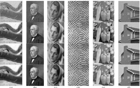
while the right column, has a zoomed version of the corresponding images in left. In order to show the performance of proposed method we zoomed on the hat region and specially focused on the oblique lines of the hat. It is obviously observable that the proposed method (with results in second row); preserves oblique line of the hat, where the other methods smooth these lines. Note that all of these methods applied with their best-tuned parameters. We have implemented the proposed method on six Gaussian noisy images with SNR=50 and the results are shown in Figure 7. The results of implementing Perona-Malik method and Catte method, with diffusion Equation (8), is also included in this figure. Subjective comparison of results shows the superiority of our proposed method to traditional PDE methods. For example, in column (a) of Figure 7, which shows a biologic tissue, the lines and edges of the image enhanced using proposed method (the second row) are sharper than the ones that were provided by the other two methods.

(a) (b) (c) (d) (e) (f)

Figure 7. (1st row), Original images distorted by Gaussian noise with SNR=50, (2nd row) results of denoising by proposed method (with a =0.06 and b=0.6 (see Figure 3)), (3rd row) Prona-Malik with diffusion Equation (8), (4th row) Catte et.al with diffusion

Equation (8).(parameters of diffusion process for (b) to (f): iteration=10, K=10, l=0.2, s2=0.2 )

(a) (b) (c) (d) (e)

Figure 8. (a) Original image, (b) noisy images with Gaussian noise (m =64 ands =400) and impulse noise (density=64).

Results of denoising by: (c) proposed method (with a =0.01 and b =1 )( (PSNR)db = (18.03)db, SSIM = 0.75, FOM = 0.68,) (d) Nadernajad’s method((PSNR)db = (11.92)db, SSIM = 0.66, FOM = 0.73,) and (e) traditional Pronal-Malik((PSNR)db = (11.73)db, SSIM = 0.53, FOM = 0.58,).

(a) (b)

4 5 6 7 8 9 10

100 200 300 400 500 600 700

s2 _{of Gaussian noise (´80)}

M

SE

MSE values for various methods

Proposed PM1 PM2 CattePM1 CattePM2

4 5 6 7 8 9 10

19 20 21 22 23 24 25 26 27 28

s2 _{of Gaussian noise (´80)}

PS

NR

PSNR values for various methods

(c) (d)

(e) (f)

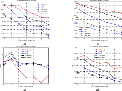
Figure 9. Values of performance measures for mentioned methods, for Gaussian noisy versions of “woman_blond.tif” with m=64

and _s2Î

320, 400, 480, 560, 640, 720 and 800, respectively, (a) MSE, (b) PSNR, (c) SSIM, (d) FOM, (e) AMBE and (f) HS.

In addition, the contrast of original image is preserved better in our algorithm results, which is the strength point in terms of image quality. We also compare performance of our proposed method with that of the state-of-the-art PDE based method proposed by Nadernejad et al. [12].

This method is a new approach based on combination of pixon concept and PDE, for image denoising. In Figure , we add a Gaussian noise, with

m=64 and s =400, in addition to impulsive noise with density = 0.15 to the test image. Figure (c) to (e) show the results of image denoising by our proposed method, Nadernejad’s method, and Perona-Malik method, respectively. Although, from the FOM perspective, the Nadernejad’s method is better, but the PSNR and SSIM values of our proposed method are the best. On the other hand, Nadernejad’s method has some impulsive noises, where the result of the proposed method is clear of them. This is an interesting property for detection-based applications like face detection. Here, we must mention that the best efficiency of our proposed method is achievable in cases, where the distorted image is not defected by enormous impulse noises.

To have an objective evaluation of the proposed method we applied it on the test image ‘woman-blonde’

for different Gaussian noises with the same m=64 but

different s2, which get their values from the set [320, 400, 480, 560, 640, 720, 800]3.Thenwecalculated the values of predefined metrics introduced in Section 4. In these experiments, the two parameters of Perona-Malik method, ‘iteration’ and ‘diffusion factor (k)’ take the same value of 10. In addition to these two parameters, the parameters l=0.2, s2₌0.2

were also set for Catte PDE method and our proposed method. Specific parameters which is used in the proposed method were,

06 . 0 =

a andb =0.6(see Figure 3), which were

determinied experimentally. For each of the image performance quantities predefined in Section 4, a chart is obtained in Figure 9. As can be seen in these charts, MSE and PSNR as two distance criteria, FOM and SSIM, as structure preserving criteria and finally AMBE and HS as brightness and contrast preserving criteria, show the better performance of proposed method in context of image distances and image quality.

7. CONCLUSIONS

We proposed a new hybrid smoothing method, which

4 5 6 7 8 9 10

0.5 0.55 0.6 0.65 0.7 0.75 0.8 0.85 0.9 0.95

s2

of Gaussian noise (´80)

FOM

FOM values for various methods

Proposed PM1 PM2 CattePM1 CattePM2

4 5 6 7 8 9 10

0.35 0.4 0.45 0.5 0.55 0.6 0.65 0.7 0.75 0.8 0.85

s2

of Gaussian noise (´80)

SS

IM

SSIM values for various methods

Proposed PM1 PM2 CattePM1 CattePM2

4 5 6 7 8 9 10

0 5 10 15 20 25

s2

of Gaussian noise (´80)

A

M

BE

AMBE values for various methods

Proposed PM1 PM2 CattePM1 CattePM2

4 5 6 7 8 9 10

0.18 0.2 0.22 0.24 0.26 0.28 0.3

s2

of Gaussian noise (´80)

HS

HS values for various methods

utilizes the Homomorphic filtering, and anisotropic diffusion concepts in the context of image denoising. In our proposed method, the reflectance and illumination components of the noisy image are extracted using a suitable Homomorphic filter and then anisotropic diffusion process is performed on each of these components separately. The major advantage of this idea, beside enhancements and contrast improvements of image, is its flexibility. Indeed, the user will be able to apply his/her enhancement method based on diffusion equation with customizable parameters on each desired component and then join them to form the final image.

8. REFERENCES

1. Gonzalez, R.C. and Woods, R.E., "Digital image processing", Prentice Hall, Vol., No., (2002), 462-463.

2. Alvarez, L., Lions, P.-L. and Morel, J.-M., "Image selective smoothing and edge detection by nonlinear diffusion. Ii", SIAM J. Numer. Anal., Vol. 29, No. 3, (1992), 845-866.

3. Perona, P. and Malik, J., "Scale-space and edge detection using anisotropic diffusion", Pattern Analysis and Machine Intelligence, IEEE Transactions on, Vol. 12, No. 7, (1990), 629-639.

4. Rudin, L.I., Osher, S. and Fatemi, E., "Nonlinear total variation based noise removal algorithms", Physica D: Nonlinear Phenomena, Vol. 60, No. 1–4, (1992), 259-268.

5. Yaroslavsky, L. and Eden, M., "Fundamentals of digital optics, Birkhäuser Boston, (1996).

6. Smith, S.M. and Brady ,J.M., "Susan&mdash;a new approach to low level image processing", Int. J. Comput. Vision, Vol. 23, No. 1, (1997), 45-78.

7. Yaroslavski, L.P., "Digital picture processing: An introduction, Springer-Verlag, (1985).

8. DONOHO, D.L. and JOHNSTONE, J.M., "Ideal spatial adaptation by wavelet shrinkage", Biometrika, Vol. 81, No. 3, (1994), 425-455.

9. Ordentlich, E., Seroussi, G., Verdu, S., Weinberger, M. and Weissman, T., "A discrete universal denoiser and its application to binary images", in Image Processing,. International Conference on. Vol. 111, (2003), 117-120

10. Farbiz, F., Menhaj, M. and Motamedi, S., "A new iterative fuzzy-based method for image enhancement", International Journal of Engineering, Vol. 13, No. 3, (2000), 69-74.

11. Alvarez, L., Lions, P.-L. and Morel, J.-M., "Image selective smoothing and edge detection by nonlinear diffusion. II", SIAM Journal on Numerical Analysis, Vol. 29, No. 3, (1992), 845-866.

12. Catté, F., Lions, P.-L ,.Morel, J.-M. and Coll, T., "Image selective smoothing and edge detection by nonlinear diffusion", SIAM Journal on Numerical Analysis, Vol. 29, No. 1, (1992), 182-193.

13. Li, X. and Chen, T., "Nonlinear diffusion with multiple edginess thresholds", Pattern Recognition, Vol. 27, No. 8, (1994), 1029-1037.

14. Whitaker, R.T. and Pizer, S.M., "A multi-scale approach to nonuniform diffusion", CVGIP: Image Understanding, Vol. 57, No. 1, (1993), 99-110.

15. Weickert, J., "Coherence-enhancing diffusion filtering", International Journal of Computer Vision, Vol. 31, No. 2-3, (1999), 111-127.

16. Gilboa, G., Sochen, N. and Zeevi, Y.Y., "Forward-and-backward diffusion processes for adaptive image enhancement and denoising", Image Processing, IEEE Transactions on, Vol. 11, No. 7, (2002), 689-703.

17. Nadernejad, E., Hassanpour, H. and Miar, H., "Image restoration using a pde-based approach", International Journal of Engineering, Transaction B: Applications, Vol. 20, No. 3, (2007), 225-236.

18. Nikpour, M. and Hassanpour, H., "Using diffusion equations for improving performance of wavelet-based image denoising techniques", IET Image Processing, Vol. 4, No. 6, (2010), 452-462.

19. Nadernejad, E. and Forchhammer, S., "Wavelet-based image enhancement using fourth order pde", in Intelligent Signal Processing (WISP), 7th International Symposium on, IEEE. (2011), 1-6.

20. Hassanpour, H. and Rostami Ghadi, A., "Image enhancement via reducing impairment effects on image components", International Journal of Engineering, Vol. 26, No. 83, (2013), 921-930.

21. Gonzalez, R.C. and Woods, R.E., "Digital image processing, Pearson/Prentice Hall, (2008).

22. Koenderink, J., "The structure of images", Biological Cybernetics, Vol. 50, No. 5, (1984), 363-370.

23. Hummel, R. and Moniot, R., "Reconstructions from zero crossings in scale space", Acoustics, Speech and Signal Processing, IEEE Transactions on, Vol. 37, No. 12, (1989), 2111-2130.

24. Rajan, J., Kannan, K. and Kaimal, M., "An improved hybrid model for molecular image denoising", Journal of Mathematical Imaging and Vision, Vol. 31, No. 1, (2008), 73-79.

25. Ling, J. and Bovik, A.C., "Smoothing low-snr molecular images via anisotropic median-diffusion", Medical Imaging, IEEE Transactions on, Vol. 21, No. 4, (2002), 377-384.

26. Nadernejad, E., "Improvement of nonlinear diffusion equation using relaxed geometric mean filter for low psnr images", Electronics Letters, Vol. 49, No. 7, ( 28 March 2013), 457-458.

27. Zhou Wang, A.C.B., "Modern image quality assessment, Synthesis lectures on image, video & multimedia processing, Morgan & Claypool Publication, (2006).

28. Z. Wang, A.C.B., H.R. Sheikh, and E.P. Simoncelli, "Image quality assessment: From error visibility to structural similarity.", IEEE Trans. Image Processing, Vol. 13, No. 4, (2004), 600-612.

29. Pratt, W.K., "Digital image processing: Piks scientific inside, Wiley, (2007).

30. John, C., "A computational approach to edge detection", IEEE Transactions on Pattern Analysis and Machine Intelligence, Vol. 8, (1986), 679-698.

Image Denoising Using Anisotropic Diffusion Equations on Reflection and

Illumination Components of Image

M. H. Khosravi, H. Hassanpour

Department of Computer Engineering, University of Shahrood, Shahrood, Iran

P A P E R I N F O

Paper history:

Received 06 January 2014

Received in revised form 13 April 2014 Accepted 22 May 2014

Keywords: Image Denoising Image Smoothing Anisotropic Diffusion Homomorphic Filtering Hybrid Image Enhancement

هﺪﯿﮑﭼ

ﺰﯾﻮﻧفﺬﺣياﺮﺑنرﺎﻘﺘﻣﺎﻧتراﺮﺣرﺎﺸﺘﻧاتﻻدﺎﻌﻣوﮏﯿﻓرﻮﻣﻮﻤﻫﺮﺘﻠﯿﻓﺮﺑﯽﻨﺘﺒﻣﺪﯾﺪﺟﯽﺒﯿﮐﺮﺗشورﮏﯾ،ﻪﻟﺎﻘﻣﻦﯾارد ﺖﺳاهﺪﺷدﺎﻬﻨﺸﯿﭘ ﺮﯾﻮﺼﺗ

.

وﯽﯾﺎﻨﺷورﮥﻔﻟﻮﻣودﻪﺑيﺰﯾﻮﻧﺮﯾﻮﺼﺗ،ﮏﯿﻓرﻮﻣﻮﻤﻫﺮﺘﻠﯿﻓزاهدﺎﻔﺘﺳاﺎﺑ يدﺎﻬﻨﺸﯿﭘشوررد

ﯿﮑﻔﺗسﺎﮑﻌﻧا ﯽﻣﮏ

دﻮﺷ

.

ﺮﺑرﺎﮐﻂﺳﻮﺗﻪﮐ،ﻪﻔﻟﻮﻣنآصﺎﺧيﺎﻫﺮﺘﻣارﺎﭘﺎﺑوﻪﻧﺎﮔاﺪﺟرﻮﻄﺑ،ﻪﻔﻟﺆﻣودﻦﯾازاﮏﯾﺮﻫﺲﭙﺳ

هﺪﺷﻒﯾﺮﻌﺗ ﯽﻣﯽﯾادزﺰﯾﻮﻧ،ﻪﺘﻓﺮﮔراﺮﻗتراﺮﺣرﺎﺸﺘﻧانرﺎﻘﺘﻣﺎﻧﻊﺑاﻮﺗﺮﯿﺛﺄﺗﺖﺤﺗ،ﺪﻧا ﺪﻧﻮﺷ

.

ﯽﯾﺎﻧاﻮﺗﻞﯿﻟﺪﺑ،ﯽﺒﯿﮐﺮﺗشورﻦﯾا

ﻪﻔﻟﺆﻣزاﮏﯾﺮﻫﮥﻨﯿﻬﺑيزﺎﺴﻬﺑردنآ ﮏﯿﮑﻔﺗ ترﻮﺼﺑﺎﻫ

رﻮﻄﺑﻪﻔﻟﺆﻣﺮﻫيراﺬﮔﺮﯿﺛﺄﺗوﺖﯿﻤﻫاﺮﺑﺪﯿﮐﺄﺗ نﺎﮑﻣاو،هﺪﺷ

ﯽﻣﻢﻫاﺮﻓارﯽﯾﻻﺎﺑﻞﻤﻋيدازآويﺮﯾﺬﭘفﺎﻄﻌﻧا،صﺎﺧ ﺪﻨﮐ

.

ومﺎﺠﻧاﺶﯾﺎﻣزآيداﺪﻌﺗ،يدﺎﻬﻨﺸﯿﭘشورﯽﺑﺎﯾزرارﻮﻈﻨﻣﻪﺑ

ﺪﺷﻪﺴﯾﺎﻘﻣوﺮﺸﯿﭘشورﻦﯾﺪﻨﭼﺎﺑنآﺞﯾﺎﺘﻧ

.

ﯽﻣنﺎﺸﻧتﺎﺸﯾﺎﻣزآﻦﯾاﺞﯾﺎﺘﻧ ﺑﺖﺒﺴﻧيدﺎﻬﻨﺸﯿﭘشورﻪﮐﺪﻨﻫد

ﻢﺘﯾرﻮﮕﻟاﻪ يﺎﻫ

ﯽﻣنﺎﺸﻧدﻮﺧزايﺮﺘﻬﺑدﺮﮑﻠﻤﻋهزﻮﺣﻦﯾاﮏﯿﺳﻼﮐ ﺪﻫد

doi: 10.5829/idosi.ije.2014.27.09c.03