Estimation and Calibration of Robot Link Parameters with
Intelligent Techniques
M. Barati*, A. R. Khoogar** and M. Nasirian***
Abstract:Using robot manipulators for high accuracy applications require precise value of the
kinematics parameters. Since measurement of kinematics parameters are usually associated with errors and accurate measurement of them is an expensive task, automatic calibration of robot link parameters makes the task of kinematics parameters determination much easier. In this paper a simple and easy to use algorithm is introduced for correction and calibration of robot kinematics parameters. Actually at several end-effecter positions, the joint variables are measured simultaneously. This information is then used in five different algorithms; least square (LS), particle swarm optimization (PSO) , Genetic algorithms (GA), quadratic particle swarm optimization (QPSO) and simulated annealing particle swarm optimization (Sa_PSO) for automatic calibration and correction of the kinematics parameters. This process was also tested experimentally via a three degree of freedom manipulator which is actually used as a coordinate measuring machine (CMM). The experimental Results prove that the intelligent algorithms are useful for both parameter identification and calibration of link parameters.
Keywords: Calibration, Identification, Genetic Algorithms, Particle Swarm Optimization,
Least Square, Robot Manipulator.
1 Introduction1
Since the introduction of the first robot manipulators in 1960s, there has always been a demand for kinematic parameters identification and subsequent error correction operations in order to improve the ability of robot manipulators in reaching a specified position consistently and accurately [1]. It has been shown that as much as 95% of robot positioning inaccuracy arises from the inaccuracy in its kinematics model description [2]. Even if it is possible to dismantle a robot manipulator and determine the parameters in detached linkages kinematic frames using accurate measuring machines, the resulting model will still contain some inaccuracies arising from joint and link compliances changing with the manipulator configurations, thermal effects, wear, joint transducer errors, steady state errors in joint positions, inaccurate knowledge of the
Iranian Journal of Electrical & Electronic Engineering, 2011. Paper first received 24 Aug. 2010 and in revised form 25 Jun. 2011. * The Author is with the Department of Electrical Engineering, Ferdowsi University, Mashhad, Iran.
E-mail: [email protected]
** The Author is with the Science and Research Branch of the Islamic Azad University, Tehran, Iran.
E-mail: [email protected]
*** The Author is with the Department of Electrical Engineering, Khaje Nasiredin Toosi University, Tehran, Iran.
E-mail: [email protected]
kinematics parameters, and payload carried by the manipulator [1].
It follows that automatic calibration of robot links parameters that can improve the manipulator accuracy will reduce the kinematics errors [3]. There is a wealth of literature on the kinematics identification and calibration of robotic systems: [2], [4], [5], [6], [7], [8].
A wide account of robot calibration consisting of (i) modeling, (ii) measurement, (iii) identification, and (iv) correction steps are available in [9] and [4].
To calibrate robotic manipulators, Everett et al. [10] presented a new kinematic model for achieving better kinematic representation. Chen and Chao [11], improve the manipulators positioning error by including the non-geometric error in kinematics model. For identification of manipulator link parameters, Stone et al. [12] have introduced the S model. Jang et al. [13] have presented a calibration methodology based on dividing the manipulator workspace into several local regions, and subsequently building a calibration equation using a three dimensional position measurement system consisting of a camera and infrared LED. Newman et al. [14] have reported on the calibration of a Motoman P-8 robot using circle point analysis technique, which requires external hardware to determine the manipulator end point positions in Cartesian space. Driels et al. [6] reported on the kinematic calibration of a PUMA 560 manipulator using a coordinate measuring machine that
provided position and orientation data for randomly selected manipulator configuration. Also for manipulator calibration, Junhong et al. [15] have used the measurement technique by coordinate measuring machine. Renders et al. [5] presented a robot kinematic parameter identification technique based on a maximum likelihood algorithm in a recursive form. Drouet et al. [16] have presented a method to compensate for the geometric and elastic errors of a six-degree of freedom medical robot. An interferometer [17] and laser tracking [14] was, also, used for manipulator endeffector position measurement. For identification of robots kinematics parameters, Horning [18] has introduced and compared four different methods. A closed-loop method has been proposed that obviates the need for pose measurement by forming a manipulator into a mobile closed-loop kinematic chain. Actually kinematics parameters are determined from the joint angle readings alone [9]. Ruibo et al. [19] presents a generic error model, which is based on the product of exponentials (POEs) formula, for serial-robot calibration.
A calibration method is presented for kinematic parameters of space manipulator by Hui Li Zhihong Jiang [20]. This method utilizes the position and orientation information of a fixed target on the space station and adopts rank-one quasi-Newton method to calculate the errors of the kinematic parameters, the position and orientation of the fixed target can be measured by the camera mounted on the manipulator’s endeffector. This method can calibrate the manipulator parameters online and has demand in working environment [20].
Calibration of a 6-PRRS parallel manipulator is studied by Yonggang Yang. et al. [21] a compensation method based on kinematic model is proposed. This method uses the D-H modeling method sets up for a 6-PRRS parallel manipulator kinematic model, it then identifies and compensates the error in model using vector chain [21].
As the above literature shows, it is virtually impossible to consider all the sources that contribute to the endeffector positioning errors in a single kinematic identification model of a robot manipulator. However, most of the positioning errors are related to the geometric parameters of linkages [2]. In this study the classical and intelligent identification techniques are used for compensation of the manipulator positioning errors which are produced by the inaccuracies of the geometric parameters. In recent years, stochastic optimization methods have gained increasing attention in parameter optimization of various systems. The most popular techniques are evolutionary computation and the simulating annealing algorithms. Since these methods do not require any gradient information, they are well suited for non-smooth or discontinuous optimization tasks occurring in nonlinear systems [22].
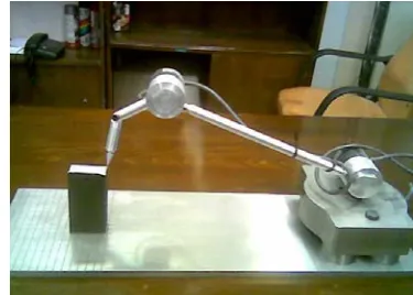
The experimental system employed here is a three degree of freedom manipulator which is actually used as
a coordinate measuring machine (CMM). Aspects of this manipulator are depicted in Fig. 1.
To model the kinematics of this manipulator, the Denavit and Hartenberg (DH) standard is used. For measurement of the joint angles, ten bit absolute encoders are used. One of the encoders is shown in Fig. 2. In order to resolve the endeffector position, the tip of the endeffector was rested against a graduated plate which has been graduated with a CNC machine with an accuracy of ± μ10 m. For identification and calibration of the geometric parameters five different methods were used. Firstly the classical least square estimation technique was employed to determine the numerical values of the kinematic parameters. Then four intelligent techniques were used.
2 Kinematics Model
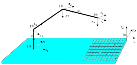
The schematic of the robot manipulator and the coordinate frames needed to generate a kinematics model are defined in Fig. 3. To model the kinematics of this manipulator, the Denavit and Hartenberg standard is used. In order to use this model, it is necessary to fix a coordinate frame to each linkage [23].
A set of possible body fixed coordinate frames is shown in Fig. 3. The DH parameters for the proposed manipulator are shown in Table 1.
These parameters are provided by the manufacture of the manipulator, in this work they are referred as the nominal parameters.
Fig. 1 The three degree of freedom manipulator.
Fig. 2 The ten bit absolute encoder.
Fig. 3 Schematic representation of the robot manipulator with links coordinate frame.
Table 1 D-H parameters for the proposed manipulator.
Joint/Link
i(deg ree)
α a (m)i d (m)i θi
1 0 -0.51 0.10
1
θ
2 -90 0 0.02
2
θ
3 0 0.31 -0.02
3
θ
e 0 0.15 0
e
θ
The homogeneous transformation matrix between two consecutive coordinate frames j and j+1, based on Devavit and Hartenberg convention, is jTj+1. With this
convention, the overall transformation matrix between the base coordinate frame and the frame fixed to the endeffector is written as
o o 1 2 3 e 1 2 3 e
T = T T T T (1)
3 Data Collection
For data collection it is necessary to measure the joint angles for each endeffector position. As mentioned earlier, for measurement of the joint angles ten bit absolute encoders are used. Encoder resolution is
351 . 0
± degree. One of the encoders is shown in Figure 2. In order to have better accuracy, encoders with higher resolutions may be used. Now for data collection, we placed the endeffector in different position of the graduated plate and took note of the encoder values.
Note that at least 4 vector measurements are needed in order to estimate the 12 specified parameters [1]. Greater number of measurements would contribute to better convergence of the algorithm and to reduce the effect of measurement noise.
4 Kinematics Parameter Identification
To find the actual value of manipulator kinematic parameters that reduce the endeffector positioning error, we must first develop the relation between the endeffector position and the kinematic parameters, i.e. the forward kinematics equations
n
P = αf ( , a, d, )θ = ϕf ( ) (2)
where Pn =
[
x y z]
T is the nominal manipulator end point position vector calculated with the nominal values of the parameters, α = α[ 0 α1 α2 α3],[
0 1 2 3]
a= a a a a , d=
[
d1 d2 d3 de]
and thejoint variables θ = θ
[
1 θ2 θ3]
. Next, the differentidentification algorithms used for this identification are described.
4.1 Nonlinear Least Square Method
Based on the nonlinear kinematic model f ( )ϕ of the manipulator expressed in (2), the kinematic parameters are estimated by minimizing the sum of the square of the 3×1 positioning error vectorΔP associated with m
number of measurements in the objective function,
m T k 1
E [ P] [ P]
=
=
∑
Δ Δ (3)where ΔP is expressed by
[
]
Tr n k
P x y z [P P ]
Δ = δ δ δ = − (4) in which P is the measured (actual) position vector, and r
x, y, z
δ δ δ are the computed position errors in the x, y, and z directions, respectively. This nonlinear least square optimization problem can be solved using either the interior-reflective Newton method or the Levenburg-Marquardt algorithm. These are two efficient optimization algorithms for large-scale nonlinear problems. It has been reported [24] that the former can solve complex nonlinear problems more efficiently than the latter. The interior-reflective Newton method employs the preconditioned conjugate gradients procedure to obtain the approximate solution of a large system of equations.
A good initial guess always helps the estimation algorithm to converge more quickly. Therefore, the nominal values of the parameters are taken as the initial guess for the parameters. The estimation techniques are realized iteratively until the position error is small enough to meet a termination condition. The position error in any particular Cartesian direction is described by the root mean square (RMS) of the position error, which is a 3×1vector.
m
2 r n i i 1
1
RMS Position (P P ) m =
− =
∑
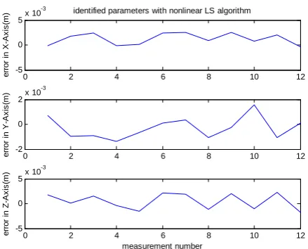
− (5)For the 12 empirically obtained data, the RMS vector was evaluated in x, y, and z directions using both the nominal values of the parameters and estimated value of the parameters via the nonlinear least square technique, and the results are summarized in Table 2. The RMS (x, y, z) indicates the evaluated errors in the x, y, and z directions and
∑
RMS is the vector length of the positioning error.Percentage of error improvement is evaluated as
Error Improvement (%) = n e
n
RMS RMS
100 RMS
− ×
(6)
where RMS is the RMS positioning error using the n
nominal parameters. And, the RMS is the RMS e
positioning error computed using the estimated parameters and element symbols.
The corresponding positioning errors in the Cartesian coordinate are shown in the Figs. 4 and 5.
Table 2 The RMS position errors with nominal and identified
parameters.
RMS (x, y, z)
∑
RMSwith nominal Par. 3
10 ] 7 . 7 6 . 10 14 . 2
[ T× − 0 .0 2 0 4
with estimated Par. 3
10 ] 6 . 1 884 . 0 7 . 1
[ T× − 0.0041
Improvement (%) T
] 22 . 79 66 . 91 56 . 20
[ 79.90
4.2 The PSO Algorithm
This algorithm begins with generation of the initial swarm of particles in which each particle moves about the cost surface with an arbitrary velocity. The particles update their velocities and positions based on the local and global best solutions [25]. If xi =(x , x ,i1 i2 , x )in
r
K and vri =(v , v ,i1 i2K, v )in are the position and velocity of the ith particle in an n dimension space, then the motion of this particle in the next step is computed as the vector sum of the present position and the velocity vectors as
k 1 k k 1 i i i
xr + =xr +vr + (7)
and, the velocity of the particle in the iteration k+1,
k 1 i
vr + , is obtained from the following equation
k 1 k k k
i i 1 i i 2 g i
v wv c rand (p x ) c rand (p x )
+ = + × r − + × r −
r r r r
(8)
where k is the iteration number, pi =(p , p ,i1 i2 , p )in
r
K is the best particle position in the ith iteration (pbest) and
g g1 g 2 gn
pr =(p , p ,K, p ) is the global best particle position
in all iterations so far (gbest), and, c and 1 c are the 2
scaling factors that determine the relative pull of pbest and gbest.
As proposed in [26], the default values of c1andc2
were selected as 2. In the standard PSO, the inertia weighting factor is quite important and it is usually chosen as a decreasing function. At the beginning it is set to winitialize =1 and finally it is reduced towfinal=0.5.
A linear relation is usually used as a function of iteration
max
initialize final final max
k k
w (w w )( ) w
k
−
= − + (9)
In the above equation k is the running step number and kmax is the maximum number of steps [22].
Next steps summarized the algorithm:
1) Generate the initial values for the particles 2) Update the positions, the velocities and the
inertia weighting factor w, in each step according to the cost function
Fig. 4 Position error of endeffector using the nominal
parameters.
Fig. 5 Position error of endeffector using the identified
parameters via nonlinear LS.
3) Repeat the loop until the desired solution is reached
We can consider a cost function for this algorithm similar to the cost function in the least square technique
m T k 1
E [ P] [ P]
=
=
∑
Δ Δ (10)In this algorithm, the nominal values of the parameters were also used as the initial value.
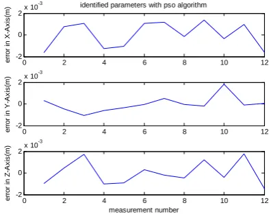
For the 12 empirically obtained data, the RMS vector was evaluated in x, y, and z directions using both the nominal values of the parameters and estimated value of the parameters via PSO algorithm. The results are summarized in Table 3.
The corresponding positioning errors in the Cartesian coordinate are shown in Figs. 6 and 7.
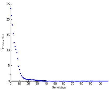
By comparing the results, we see that the PSO algorithm performs better. Also in this algorithm, the value of the fitness function for the best individual in each generation is shown in Fig. 8.
0 2 4 6 8 10 12
-5 0 5x 10
-3
er
ror i
n
X
-A
x
is
(m
) nominal parameters
0 2 4 6 8 10 12
-0.015 -0.01 -0.005
e
rr
o
r i
n
Y-Ax
is
(m
)
0 2 4 6 8 10 12
0 0.005 0.01 0.015
e
rr
o
r in
Z
-A
x
is
(m
)
measurement number
0 2 4 6 8 10 12
-5 0 5x 10
-3
error i
n
X
-A
x
is
(m
) identified parameters with nonlinear LS algorithm
0 2 4 6 8 10 12
-2 0 2x 10
-3
e
rro
r i
n
Y
-A
x
is
(m
)
0 2 4 6 8 10 12
-5 0 5x 10
-3
error i
n
Z
-A
x
is
(m
)
measurement number
Table 3 The RMS position errors with nominal and identified parameters by PSO algorithm.
RMS(x, y, z)
∑
RMSWith nominal par. T 3
[2.14 10.6 7.7] ×10− 0.0204
With estimated par. T 3
[1.1 0.673 1.1] ×10− 0.0028
Improvement (%) T
[48.6 93.65 85.71] 86.27
Fig. 6 Position error of endeffector using the nominal
parameters.
Fig. 7 position error of endeffector using the identified
parameters via PSO algorithm.
Fig. 8 The value of fitness function per iteration.
4.3 Genetic Algorithm
Genetic algorithms operate based on the theory of evolution in the nature, i.e., the algorithms search for a best solution from the population of potential solutions. In every generation, the better individuals are selected. Successive populations are generated through reproduction, crossover and mutation. In this process, better individuals reproduce in the next generation with a greater probability [27].
When the algorithm begins, the initial population is generated randomly and the fitness of each individual is evaluated from the cost function. If the termination condition is not reached, choose the parents of the next generation based on their fitness functions. The next generation is produced through crossover between parents of the previous generation. A mutation operator is also included. This process is continued iteratively until the desired termination condition is reached [29].
Consider a cost function for this algorithm similar to the cost function used in the least square technique. In this algorithm, the nominal values of the parameters were also used as the initial value.
For the 12 empirically obtained data, the RMS vector was evaluated in x, y, and z directions using both the nominal values of the parameters and estimated value of the parameters via Genetic algorithm, and the results are summarized in Table 4.
The corresponding positioning errors in the Cartesian coordinate are shown in Figs. 9 and 10.
The value of the fitness function for the best individual in each generation is shown in Fig. 11.
Table 4 The RMS position errors with nominal and identified
parameters via Genetic algorithm.
RMS(x, y, z)
∑
RMSWith nominal Par. T 3
[2.14 10.6 7.7] ×10− 0.0204
With estimated Par. T 3
[1.2 0.725 1.3] ×10− 0.0033
Improvement (%) T
[43.92 93.16 83.11] 83.82
4.4 The QPSO algorithm
The QPSO algorithm is a simple and modified integrated version of basic PSO (BPSO) and EA. The quadratic crossover operator suggested in [31] is a nonlinear multi parent crossover operator which makes use of three particles (parents) of the swarm to produce a particle (offspring) which lies at the point of minima of the quadratic curve passing through the three selected particles. The nonlinear nature of the quadratic crossover operator used in this work helps in finding a better solution in the search space.
2 2 2 2 2 2
i i i i i i
i
i i i i i i
1 (b c ) f (a) (c a ) f (b) (a b ) f (c) x
2 (b c ) f (a) (c a ) f (b) (a b ) f (c)
− × + − × + − ×
= ×
− × + − × + − ×
%
(11) The computational steps of the QPSO algorithm are given below:
0 2 4 6 8 10 12
-5 0 5x 10
-3
er
ro
r i
n
X
-A
x
is
(m
) nominal parameters
0 2 4 6 8 10 12
-0.015 -0.01 -0.005
er
ro
r i
n
Y
-A
x
is
(m
)
0 2 4 6 8 10 12
0 0.005 0.01 0.015
e
rr
o
r i
n
Z
-A
x
is
(m
)
measurement number
0 2 4 6 8 10 12
-2 0 2x 10
-3
e
rro
r i
n
X
-A
x
is
(m
) identified parameters with pso algorithm
0 2 4 6 8 10 12
-2 0 2x 10
-3
e
rr
o
r i
n
Y-Ax
is
(m
)
0 2 4 6 8 10 12
-2 0 2x 10
-3
er
ror
i
n
Z
-A
x
is
(m
)
measurement number
0 50 100 150 200 250 300 350 400
0 0.5 1 1.5 2 2.5 3 3.5 4 4.5x 10
-4
iteration
fi
tnes
s
f
unc
ti
on
Fig. 9 Position error of endeffector using the nominal parameters.
Fig. 10 Position error of endeffector using the identified
parameters via Genetic algorithm.
Fig. 11 The value of fitness function per generation.
1-Initialize the swarm 2-For each particle Update velocity Update position Update personal best
Update global best
3-Find a new particle using equation (11)
4-Replace the worst Particle by the new Particle While (Stopping condition is not reached), [31].
We can consider a cost function for this algorithm similar to the cost function in the least square technique. In this algorithm, the nominal values of the parameters were also used as the initial value.
For the 12 empirically obtained data, the RMS vector was evaluated in x, y, and z directions using both the nominal values of the parameters and estimated value of the parameters via QPSO algorithm, and the results are summarized in Table 5.
The corresponding positioning errors in the Cartesian coordinate are shown in Figs. 12 and 13.
Table 5 The RMS position errors with nominal and identified
parameters via QPSO algorithm.
RMS(x, y, z)
∑
RMSWith nominal Par. T 3
[2.14 10.6 7.7] ×10− 0.0204
With estimated Par. T 3
[1.1 0.69 1.1] ×10− 0.0029
Improvement (%) T
[47.06 93.43 85.76] 85.67
4.5 The Sa-PSO Algorithm
The idea of simulated annealing algorithm is presented by Metropolis in 1953, and was used in compounding optimization by Kirkpatrick in 1983. It accepts the current optimal solution at a probability after searching, which called Metropolis law. And Sa-PSO algorithm become a global optimal algorithm by using this new acceptance rule, the theory has been proved [32]. The basic idea of simulated-annealing particle swarm optimize algorithm (Sa-PSO) is shown below.
At the beginning, the individual best point and the global best point were accepted by the Metropolis rule, the hypo-best point was accepted at probability, the aim function is allowed to become worse at a certain extent, the acceptance rule was decided by the coefficient T, where T is the anneal temperature. With the T descending, the searching region would be around the best point, the accepted probability of the hypo-best point become small also, when the T descend to the lower limit, the accepted probability of the hypo-best point is zero, the algorithm only accept the best solution as the basic PSO algorithm. The relation between the annealing temperature and the inertial weight was built, the inertial weight changes with the temperature, and then the searching precision was changed following the inertial weight, so the searching speed was increased [31].
i
f (x ) is the ith particle solution, p ii s the historical
best solution, Tis the annealing temperature. The steps of Sa-PSO are shown below:
0 2 4 6 8 10 12
-5 0 5x 10
-3
e
rror i
n
X
-A
x
is
(m
) nominal parameters
0 2 4 6 8 10 12
-0.015 -0.01 -0.005
e
rror i
n
Y
-A
x
is
(m
)
0 2 4 6 8 10 12
0 0.005 0.01 0.015
erro
r i
n
Z
-A
x
is
(m
)
measurement number
0 2 4 6 8 10 12
-5 0 5x 10
-3
e
rr
o
r i
n
X-Ax
is
(m
) identified parameters with genetic algorithm
0 2 4 6 8 10 12
-5 0 5x 10
-3
e
rr
o
r i
n
Y-Ax
is
(m
)
0 2 4 6 8 10 12
-5 0 5x 10
-3
e
rr
o
r in
Z
-A
x
is
(m
)
measurement number
Fig. 12 Position error of endeffector using the nominal parameters.
Fig. 13 Position error of endeffector using the identified
parameters via QPSO algorithm.
Step 1: Initialize the coefficients, This includes the annealing temperature T and w, c , c1 2. To initialize the particle swarm, it includes the particle random position and the first speed;
Step 2: Evaluate each particle’s adaptive value f (x )i ;
Step 3: For each particle, the adaptive value f (x ) i is
compared with one of the historical best position p i if
the adaptive value is better than one of pi. Then, x i is
consider as the best position p ,i otherwise, using the
accept-probability law function (12) to decide if this point is accepted.
P exp(= −Δf / T) (12)
Setp 4: For each particle, the best point pi itself was
compared with the whole best point pg, if pi is better
than pg, then reset pg, otherwise, the global point is
acceted according to the probability function (12).
Step 5: The position and speed of each particle were changed following functions (7) and (8) (The functions
(7) and (8) define the basic PSO algorithm)[33], several steps later, in order to adjust the temperature T and the inertial weight w, the functions presented in (13) and (14) can be used.
1/ N
k 0
T(k)= αT (13)
0 0
0
T T(k)
w w (1 )
T
−
= −
β× (14)
Step 6: if the desired condition is not satisfied, then go back to step 2, otherwise stop.
Consider a cost function for this algorithm similar to the cost function used in the least square technique. In this algorithm, the nominal values of the parameters are also used as the initial value.
For the 12 empirically obtained data, the RMS vector was evaluated in x, y, and z directions using both the nominal values of the parameters and estimated value of the parameters via Sa-PSO algorithm, the results are summarized in Table 6.
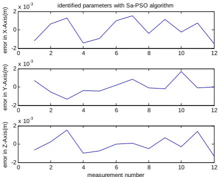
The corresponding positioning errors in the Cartesian coordinate are shown in Figs. 14 and 15.
Fig. 14 Position error of endeffector using the nominal
parameters.
Fig. 15 Endeffector position error using the identified
parameters via the Sa-PSO algorithm.
0 2 4 6 8 10 12
-5 0 5x 10
-3
er
ror i
n
X
-A
x
is
(m
) nominal parameters
0 2 4 6 8 10 12
-0.015 -0.01 -0.005
e
rr
o
r i
n
Y-Ax
is
(m
)
0 2 4 6 8 10 12
0 0.005 0.01 0.015
e
rr
o
r in
Z
-Ax
is
(m
)
measurement number
0 2 4 6 8 10 12
-2 0 2x 10
-3
e
rro
r i
n
X
-A
x
is
(m
) identified parameters with QPSO algorithm
0 2 4 6 8 10 12
-2 0 2x 10
-3
e
rr
o
r i
n
Y-Ax
is
(m
)
0 2 4 6 8 10 12
-2 0 2x 10
-3
e
rr
o
r in
Z-A
x
is
(m
)
measurement number
0 2 4 6 8 10 12
-5 0 5x 10
-3
erro
r i
n
X
-A
x
is
(m
) nominal parameters
0 2 4 6 8 10 12
-0.015 -0.01 -0.005
e
rr
o
r in
Y
-Ax
is
(m
)
0 2 4 6 8 10 12
0 0.005 0.01 0.015
er
ror i
n
Z
-A
x
is
(m
)
measurement number
0 2 4 6 8 10 12
-2 0 2x 10
-3
e
rro
r i
n
X
-A
x
is
(m
) identified parameters with Sa-PSO algorithm
0 2 4 6 8 10 12
-2 0 2x 10
-3
e
rro
r i
n
Y
-A
x
is
(m
)
0 2 4 6 8 10 12
-2 0 2x 10
-3
er
ro
r i
n
Z
-A
x
is
(m
)
measurement number
Table 6 The RMS value of position errors with nominal and identified parameters via Sa-PSO algorithm.
RMS(x, y, z)
∑
RMSWith nominal Par. 3
10 ] 7 . 7 6 . 10 14 . 2
[ T× − 0.0204
With estimated Par. T 3
[1.1 0.74 0.85] ×10− 0.0027
Improvement (%) T
[49.22 92.97 88.92] 86.85
Table 7 The Nominal and Identified parameters using the LS
method.
Identified parameters Nominal L S
0
a (cm) -51 - 51.62
1
a (cm) 0 1.5
2
a (cm) 31 31.14
3
a (cm) 14 14.99
0(deg ree)
α 0 0.2521
1(deg ree)
α -90 -88.9286
2(deg ree)
α 0 -3.9534
3(deg ree)
α 0 -9.683
1
d (cm) 10 10.1
2
d (cm) 2 1.91
3
d (cm) -2 -1.89
e
d (cm) 0 1.12
Iteration -- 5 Final value of the
fitness function
-- 5
10 4 . 3 × −
Elapsed time of the algorithm
-- 1.039 Sec
Table 8 The Identified parameters using the Genetic
Algorithm and Particle Swarm Optimization.
Identified par. PSO GA
0
a (cm) -52.12 -52.10
1
a (cm) 0.38 7.03
2
a (cm) 30.91 30.53
3
a (cm) 15.37 14.34
0(deg ree)
α 0.8422 0.8422
1(deg ree)
α -89.9885 -87.3578
2(deg ree)
α -4.1138 -4.1769
3(deg ree)
α 0.1604 2.6643
1
d (cm) 10.20 10.25
2
d (cm) 2.37 3.11
3
d (cm) 1.3 -2.10
e
d (cm) 0.25 -0.21
Iteration 400 800
Final value of the fitness function
6
10 68 .
0 × − 6
10 11 . 5 × −
Elapsed time of the algorithm
3.65 Sec 3.21 Sec
Nominal parameters and Identified parameters using the Least Square technique are summarized in Table 7.
The Identified parameters using the Genetic Algorithm and Particle Swarm Optimization are summarized in Table 8.
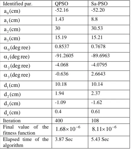
Identified parameters using the QPSO Algorithm and Sa-PSO Algorithm are summarized in Table 9.
Table 9 Identified parameters using the QPSO Algorithm and
Sa-PSO Algorithm.
Identified par. QPSO Sa-PSO
0
a (cm) -52.16 -52.20
1
a (cm) 1.43 8.8
2
a (cm) 30 30.53
3
a (cm) 15.19 15.21
0(deg ree)
α 0.8537 0.7678
1(deg ree)
α -91.2605 -89.6963
2(deg ree)
α -4.068 -4.0795
3(deg ree)
α -0.636 2.6643
1
d (cm) 10.18 10.14
2
d (cm) 1.94 2.37
3
d (cm) -1.09 -1.62
e
d (cm) 0.4 0.61
Iteration 400 108
Final value of the fitness function
6
10 68 .
1 × − 8.11×10⁻⁶
Elapsed time of the algorithm
3.87 Sec 5.43 Sec
5 Conclusions
In this study, the classical technique of the least square and four intelligent algorithms i.e. genetic algorithms, particle swarm optimization algorithm, QPSO and Sa-PSO was used for identification and calibration of a manipulator kinematics parameters. Numerical and experimental results demonstrate that these techniques are effective in reduction of positioning error.
Advantages of using intelligent methods in comparison with classical calculus based methods are,
• They do not require complex derivative evaluations
• Their applications are simple
• They don’t get caught in local minima as easily as the classic method
The obvious advantage of the proposed algorithm is that it does not require very advance equipments for data collection. Inexpensive experimental devices can be used to obtain valuable kinematic parameters. The proposed algorithms were able to compensate as much as 87% of the positioning error.
Using other objective functions in the intelligent methods may improve the identification results.
Using better encoders with higher resolutions can improve the algorithms performance. Other sources of
error, thermal errors, joint transducer errors, steady state errors in the joint positions and …, can be incorporated in the calibration model in future works.
References
[1] Alici G. and Shirinzadeh B., “A Systematic technique to estimate positioning errors for robot accuracy improvement using laser interferometry based sensing”, Elsevier Journal of Mechanism and Machine Theory, Vol. 40, No. 8, pp. 879-906, 2005.
[2] Zhong X. L. and Lewis J. M., “A New Method for Autonomous Robot Calibration”, IEEE Int. Conf. on Robotic and Automation, pp. 1790-1795,
1995.
[3] Abderrahim M., Khamis A., Garrido S. and Moreno L., Accuracy and Calibration Issues of Industrial Manipulators, Industrial Robotics: Programming, Simulation and Application, Edited by: Low Kin Huat. Germany, 2006. [4] Roth Z. S., Mooring B. W. and Ravani B., “An
Overview of Robot Calibration”, IEEE Journal of Robotics and Automation, Vol. 3, No. 5, pp. 377-384, 1987.
[5] Renders J. M., Rossignol E., Becquet M. and Hanus R., “Kinematic Calibration and Geometrical Parameter Identification for Robots”,
IEEE Transactions on Robotics and Automation, Vol. 7, No. 6, pp. 721-732, 1991.
[6] Driels M. R., Swayze W. and Potter U. S., “Full-pose calibration of a robot manipulator using a coordinate-measuring machine”, International Journal of Advanced Manufacturing Technology, Vol. 8, No. 1, pp. 34-41, 1993.
[7] Alici G. and Shirinzadeh B., “Laser
interferometry based robot position error modeling for kinematic calibration”, Proc. IEEE Int. Conf. Intelligent Robots and Systems, pp. 3588-3593, 2003.
[8] Hayati S. A., “Robot arm geometric link
parameter estimation”, Proc. 22th IEEE Decision and Control Conf., pp. 1477-1483, 1983.
[9] Maric P. and Potkonjak V., “Geometrical
Parameter Estimation for Industrial Manipulators Using Two-step Estimation Schemes”, Journal of intelligent and Robotic System, Vol. 24, No. 1, pp. 89-97, 1999.
[10] Everett L., Driels M. and Mooring B., “Kinematic Modeling for Robot Calibration”, IEEE Int. Conf. on Robotic and Automation, pp. 183-189, 1987. [11] Chen J. and Chao L. M., “Positioning Error
Analysis for Robot Manipulator with all Rotary Joints”, Pro. IEEE Int. Conf. on Robotics and Automation, pp. 1011-1016, 1986.
[12] Stone H. W., Sanderson A. C. and Neumann C. P., “Arm Signature Identification”, Proc. IEEE Int. Conf. on Robotics and Automation, pp. 41-47, 1986.
[13] Jang J. H., Kim S. H. and Kwak Y. K.,
“Calibration of geometric and non-geometric errors of an industrial robot”, Robotica, Vol. 19, pp. 311-321, 2001.
[14] Newman W. S., Birkhimer C. E., Horning R. J. and Wilkey A. T., “Calibration of a Motoman P8 robot based on laser tracking”, Proc. IEEE Int. Conf. on Robotics and Automation, pp. 3597-3602, 2000.
[15] Junhong J., Lining S. and Lingato Y., “A New Pose Measuring and Kinematics Calibration Method for Manipulators”, IEEE Int. Conf. on Robotic and Automation, pp. 4925-4930, 2007.
[16] Drouet P., Dubowsky S., Zeghloul S. and
Mavroidis C., “Compensation of geometric and elastic errors in large manipulators with an application to a high accuracy medical system”,
Robotica, Vol. 20, No. 3, pp. 341-352, 2002.
[17] Newman W. S. and Osborn D. W., “A New
Method for Kinematic Parameter Calibration via Laser Line Tracking”, IEEE Int. Conf. on Robotic and Automation, Vol. 2, pp. 160-165, May 1993.
[18] Hayati S. A., “Robot arm geometric link
parameter estimation”, Proc. 22th IEEE Decision and Control Conf., pp. 1477-1483, 1983.
[19] Ruibo H., Yingjun Z., Shunian Y., Shuzi Y., “kinematic-Parameter Identification for Serial-Robot Calibration Based on POE Formula”, IEEE Transactions on Robotics, Vol. 26, No. 3, pp. 411-423, 2010.
[20] Hui L., Zhihong J. and Qiang Huang Y. H., “Vision-based space manipulator online self-calibration ”, IEEE International conference on Robotics and Biomimetics (ROBIO), pp. 1768-1772, 2009.
[21] Yonggang Y., Yubin L., Yongsheng P. J. and Shi W. L., “An Calibration of a 6-PRRS parallel manipulator using D-H method combined with vector chain”, International Conference on Mechatronics and Automation ( ICMA), 2009. [22] Sadoghi H. and Effati S., “Eigenvalue Spread
Criteria in the Particle Swarm Optimization algorithm for Solving of Constraint Parametric Problem”, Elsevier Journal of Mathematics and computation, Vol. 192, No. 1, pp. 40-50, 2007. [23] Graig J. J., Introduction to Robotics,
Addition,-Weseley, 2nd edition, 1989.
[24] Coleman T. F. and Li L., “An interior, trust region approach for nonlinear minimization subject to bounds”, Journal of Optimization, Vol. 6, No. 1, pp. 418-445, 1996.
[25] Kennedy J. and Eberhart R., “Particle Swarm Optimization”, Proc. IEEE Int. Conf. Neural Network, pp. 1942-1948, 1995.
[26] Kennedy J., Eberhart R. and Shi Y., Swarm Intelligence, Morgan Kaufman Publishers, USA, 2001.
[27] Poorza
artifici
Neday 2006. [28] Ali M Global Opera pp. 17 [29] Zahiri “Intell Classif Electro pp. 1-9 [30] Lucas Z., “M Linear Particl Journa (IJEEE
[31] Pant R Algori Optim Hybrid pp. 21 [32] Chaoju Optim ofSimu Journa Securi [33] Lucas F., “U Design Magne Optim Electri Vol. 6
aker S. A.,
ial neural ne
ye Sabze Sho
M. M. and To l Optimizatio
ations Researc
03-1725, Sept S., Rajabi M ligent and Rob
fier”, Iranian onic Engineer
9, 2005. C., Tootoon Multi-Objectiv r BrushlessPer le Swarm O
al of Electric E), Vol. 6, No R. and Than ithm with Cr mization Probl
d Intelligent S
5-222, 2007. un D. and mization Algo
ulated Annea
al of Comp ity, Vol. 6, No C., Nasiri-G Using Modul n Optimizati et Synchrono mization (PS
ical & Elec
, No. 4, pp. 21
Artificial i etwork & alg
omal Publish
orn A. “Popul on Algorithms
ch journal. V t 2004. ashhadi H. an bust Genetic A
n Journal o ring (IJEEE), nchian F. and ve Design Op
rmanent Mag Optimization
cal & Electr
o. 3, pp. 183-1 ngaraj A. A. rossover Ope ems” Springe Systems (ASC)
Zulian Q., “ orithm Based aling”, IJCSN puter Science
o.10, pp. 152-1 Gheidari Z. an lar Pole for
on of a Li ous Motor by
O)”, Irania tronic Engin
14-223, 2010.
intelligence a gorithm gene
her, 1th editi
lation Set Ba s”, Computer
Vol. 31, No.
nd Seyedin S. Algorithm Ba
of Electrical
, Vol. 1 , No
d Nasiri-Gheid ptimization o gnet Motor Us (PSO)”, Iran ronic Enginee
89, 2010. , “A new P rator for Glo
er Innovations ), Vol. 44, No “Particle Swa d on the I
NS Internatio e and Netw
157 ,Oct. 2006 nd Tootoonch Multi-object inear Perman yParticle Swa an Journal neering (IJEE and etic, ion. ased r & 10, A., ased & o. 3, dari of a sing nian erin PSO obal s in
. 1 ,
arm Idea onal work 6. hian tive nent arm of EE), in and Lab Pro Pub “Co boo res ran and Vib afte now now rob Sairan Spatial
d he is also t boratory. He ha ogram’s Thesis blished over 4 ontrol System ok “Flight Dy
earch interests nging from robo d optimization brations.
er that he wor w. He has Publi w. His researc botics. Maryam Sabzevar received Ferdows in 2006. engineer is inte techniqu intereste l Industrial Gr
Ahmad
degrees Alabama Robotics that he w Branch Space S He is cu in the S of the A the director of as supervised m
and dissertatio 40 technical p
Design Using ynamics” to t span a broad otics, Intelligen n in autonom
Mehrzad degree fro and techn graduated engineerin Toosi in Search Si until 1996 didactic defence m rks in Sairan S
ished 17 techni ch interests to
m Barati w
r, Iran in her B.S d si University She graduate ring in M.S i
erested in ue and Sh
d in Robotic roup until now
R. Khoogar r
from The U a including a Ph s and Control i worked in the of the MacDon System Compan urrently a Assis
cience and Res Azad Universi f an Industria more than 40 M ons during this
apers, Authore Matlab” and T the Persian la interdisciplina nt System learn mous systems
d Nasirian re
om Iran Univer nology (IUST) d in Ph.D. deg ng from Kh n 2007. He w
ite in surface ef 6. After that he and Research ministry from 1 Spatial Industri cal papers and satellite, groun
was born in 1984. She degree from
of Mashhad ed in Control
n 2008. She intelligent e is also . She works w.
received three University of
h.D. degree in in 1989. After Space System nnell Douglas ny until 1991. stant Professor
search Branch ity in Tehran al Automation MS and Ph.D.
time. He has ed a book in Translated the anguage. His ary curriculum
ning, planning to Industrial
ceived his M.S rsity of science ) in 1995. He gree in Control haje Nasiredin worked in the ffect from 1993 e worked in the institution of 999 until 2003 ial Group until 3 journals until nd station and S e e l n e e f l l d