AN OPTIMIZED ONLINE SECONDARY PATH MODELING
METHOD FOR SINGLE-CHANNEL
FEEDBACK ANC SYSTEMS
P. Davari and H. Hassanpour*
School of Information Technology and Computer Engineering, Shahrood University of Technology P.O. Box 316, Shahrood, Iran
[email protected] - [email protected]
*Corresponding Author
(Received: September 10, 2007 – Accepted in Revised Form: September 25, 2008)
Abstract This paper proposes a new method for online secondary path modeling in feedback active
noise control (ANC) systems. In practical cases, the secondary path is usually time-varying. For these cases, online modeling of secondary path is required to ensure convergence of the system. In literature the secondary path estimation is usually performed offline, prior to online modeling, where in the proposed system there is no need for using offline estimation. The proposed method consists of two steps: a noise controller which is based on an FxLMS algorithm, and a variable step size (VSS) LMS algorithm which is used to adapt the modeling filter with the secondary path. In order to increase performance of the algorithm in a faster convergence and accurate performance, we stop the VSS-LMS algorithm at the optimum point. The results of computer simulation shown in this paper indicate effectiveness of the proposed method.
Keywords Active Noise Control, Adaptive Filter, Feedback, FxLMS, Secondary Path, Online
Modeling
ﻩﺪﻴﻜﭼ
ﺍﺭﺩ ﻳ ﺪﺟﺵﻭﺭ ﻪﻟﺎﻘﻣﻦ ﻳﺪ ﻱ ﻝﺪﻣ ﺖﻬﺟ ﺯﺎﺳ ﻱ ﻧﺁ ﻲ ﺴﻣ ﻴﺮ ﻮﻧﺎﺛ ﻳ ﺍﺮﺑﻪ ﻱ ﺳ ﻴ ﻢﺘﺴ ﺎﻫ ﻱ ﻮﻧﻝﺎﻌﻓ ﻝﺮﺘﻨﮐ ﻳﺰ
ﺎﺑ
ﺲﭘﺭﺎﺘﺧﺎﺳ ﺩﺭﻮﺧ
ﺖﺳﺍ ﻩﺪﺷﻪﺋﺍﺭﺍ . ﺴﺑﺭﺩ ﻴ ﺭﺎ ﻱ ﺎﻫﺩﺮﺑﺭﺎﮐﺯﺍ ﻪﮐ ﺴﻣ ﻴﺮ ﻮﻧﺎﺛ ﻳ ﻐﺘﻣﻪ ﻴ ﻥﺎﻣﺯﺎﺑﺮ ﺖﺳﺍ ، ﺍﺮﺑ ﻱ ﻤﻃﺍ ﻴ ﺯﺍﻥﺎﻨ ﺍﺮﮕﻤﻫ ﻲﻳ ﺳ ﻴ ﻧﻢﺘﺴ ﻴ ﻝﺪﻣﻪﺑﺯﺎ ﺯﺎﺳ ﻱ ﻧﺁ ﻲ ﺴﻣ ﻴﺮ ﻮﻧﺎﺛ ﻳ ﻣﻪ ﻲ ﺪﺷﺎﺑ . ﺭﺩ ﺵﻭﺭ ﻩﺪﺷﻪﺋﺍﺭﺍ ﺵﻭﺭﻑﻼﺧﺮﺑ ﺎﻫ ﻱ ﻪﮐﻪﺘﺷﺬﮔ ﻤﺨﺗﺯﺍ ﻴ ﻏﻦ ﻴ ﻧﺁﺮ ﻲ ﻣﻩﺮﻬﺑ ﻲ ﮔﻴ ﺪﻧﺮ ،ﻧ ﻴ ﺯﺎ ﻱ ﻨﭼﺯﺍﻩﺩﺎﻔﺘﺳﺍﻪﺑ ﻴ ﻤﺨﺗﻦ ﻴﻨ ﻲ ﺩﺭﺍﺪﻧﺩﻮﺟﻭ . ﺳ ﻴ ﺯﺍﻩﺪﺷﻪﺋﺍﺭﺍﻢﺘﺴ ﻳ
ﮏ ﻝﺮﺘﻨﮐ
ﻮﻧﻩﺪﻨﻨﮐ ﻳ ﺎﻨﺒﻣﺮﺑﻪﮐﺰ ﻱ FxLMS ﻭ ﻳ ﻝﺪﻣﮏ ﺴﻣﻩﺪﻨﻨﮐ ﻴﺮ ﻮﻧﺎﺛ ﻳ ﺭﻮﮕﻟﺍﺱﺎﺳﺍﺮﺑﻪﮐﻪ ﻳ ﻢﺘ VSS-LMS ﻞﻤﻋ ﻣ ﻲ ﺪﻨﮐ ﮑﺸﺗ ﻴ ﺖﺳﺍ ﻩﺪﺷ ﻞ .
ﺩ ﭘ ﺵﻭﺭ ﺭ ﻴ ﺩﺎﻬﻨﺸ ﻱ ﺍﺮﺑ ﻱ ﺍﺰﻓﺍ ﻳ ﺍﺮﮕﻤﻫ ﺶ ﻲﻳ ﻫﺩﺯﺎﺑﻭ ﻲ ﺭﻮﮕﻟﺍ ﻳ ﻢﺘ ﻝﺪﻣ ، ﺯﺎﺳ ﻱ ﻪﻄﻘﻧ ﺭﺩ ﺍ ﻱ ﻬﺑ ﻴ ﻣﻒﻗﻮﺘﻣﻪﻨ ﻲ ﺩﻮﺷ . ﺒﺷ ﻴﻪ ﺯﺎﺳ ﻱ ﺎﻫ ﻱ ﻣﻥﺎﺸﻧﺍﺭﻩﺪﺷﻪﺋﺍﺭﺍﺵﻭﺭﻥﺩﻮﺑﺮﺛﺆﻣﻩﺪﺷﻪﺋﺍﺭﺍ ﻲ
ﺪﻨﻫﺩ .
1. INTRODUCTION
Acoustic noises have become a serious problem by the wide spread use of industrial equipment such as: fans, engines, compressors, and transformers. Active noise control (ANC) is an electro acoustic system that efficiently attenuates low frequencies unwanted noises (primary noise) where passive methods are either ineffective or tend to be very expensive or bulky. An anti-noise of equal amplitude and opposite phase the replica of the primary noise was generated, and then combined with the unwanted disturbance
(d(n) in Figure 1). Following the superposition principle, the result was the cancellation or reduction of both noises [1].
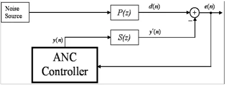
Figure 1. Block diagram of feedback ANC system.
is the reason that significant ANC improvements are mainly taken place in using feed-forward structure [2-7]. However, feedback structure has some especial applications where using feed-forward is impractical. This happens when the reference sensor in the ANC system is unachievable or impracticable. One of the most important applications of the feedback structure is ANC headphones [8-11].
The block diagram of feedback ANC system [1,8,11] is shown in Figure 1. Here, P(z) is the primary path consists of the acoustic response from the reference noise source to the error sensor, and S(z) is the secondary path which includes digital-to-analog (D/A) converter, reconstruction filter, amplifier, loudspeaker, acoustic path from loudspeaker to error sensor (microphone), error sensor, preamplifier, antialiasing filter, and analog-to-digital (A/D) converter [12]. The secondary path is practically time varying and introduces delay. These characteristics cause instability problem to the standard Least Mean Square (LMS) algorithm, resolving the instability problem requires using FxLMS algorithm [1,10,13]. The FxLMS algorithm uses estimation of the secondary path to overcome the problem raised by the above-mentioned characteristics of the secondary path. Estimation of the secondary path is performed offline prior to the implementation of ANC algorithm, but in practical cases the secondary path are usually time varying. Consequently, online modeling of secondary path is required to ensure the convergence of the ANC algorithm [2-7]. In ANC systems, there are two different methods for online secondary-path modeling. The first approach utilizes a system identification method to model the secondary path, which
introduces the injection of additional random noise into the ANC system. The second approach attempts to model the path from the output of the ANC controller to avoid the injection of additional random noise into the ANC system. However, the comparison results of these two online modeling approaches indicates that the first approach is superior to the second, on convergence rate, the primary noise response changes speed, updating duration, computational complexities, etc. [2]. Although injection of additional random noise may cause the system to be unstable, especially in a feedback structure; it provides an appropriate estimation of the secondary path. On the other hand, using the output of the ANC controller in calculating the secondary path always provides a stable system [8]. Hence, we tend to use the overall advantages of both approaches in this research. Consequently, in order to increase the performance of the proposed ANC system, we use the injection of the additional random noise in secondary path estimator algorithm, to have an appropriate estimation of this path. To prevent instability problem of using random noise, the algorithm of secondary path calculator is stopped at the optimum point. Additionally, estimation of secondary path is usually performed offline, followed by online modeling, where in our algorithm there is no need to use offline estimation of this path.
The proposed method is based on an FxLMS algorithm which acts as the main part of the system, and a variable step size (VSS) LMS algorithm [3,4] which is used to adapt the modeling filter with secondary path. The main reason that we implement our algorithm on feedback structure is to solve instability problem with this structure in some circumstances such as industrial application like ANC headphones. Although more stable, implementation of the ANC system using feed-forward structure is impractical in such applications.
The rest of the paper is organized as follows. In Section 2, feedback ANC system is briefly described. Section 3 introduces our proposed method. In Section 4 we illustrate our simulation results, and finally in Section five conclusions are drawn.
2. FEEDBACK ANC SYSTEM
As it was mentioned before, transfer function of the secondary path is crucial in generating anti-noise in ANC applications as it is time varying and introduces delay, causing instability problem to the standard LMS algorithm. The instability problem can be resolved using the FxLMS algorithm [1,8]. The FxLMS algorithm uses estimation of the secondary path to overcome the problems of the secondary path [1]. This algorithm can be applied to both feedback and feed-forward structures [1]. The block diagram of a feedback FxLMS ANC system [11] is shown in Figure 2. In this figure
) z (
Sˆ is the estimation of secondary path S(z). Unlike feed-forward structure, a reference sensor is available to pick the reference signal x(n), the main problem of implementing the feedback ANC system is to estimate the primary noise (d(n)) and use it as a reference signal for the ANC filter (W(z)) [11].
As Figure 2 shows, the reference signal x(n) is a summation of two signals e(n) and yˆ′(n) [10]:
∑−
= −
+ =
≡ M 1
0 m ) m n ( y m sˆ ) n ( e ) n ( dˆ ) n (
x (1)
Where sˆm represent coefficients of the M th order FIR filter Sˆ(z). In this figure, the secondary signal y(n) is generated as:
Y(n) = WT(n)X(n) (2)
Where W(n) and X(n) are the coefficient and signal vectors of length L, the order of the FIR filter W(z), at time n. These coefficients updated by the FxLMS algorithm as follows:
) n ( e ) 1 n ( x ) n ( l w ) 1 n ( l
w + = +μ ′ −
1 L ,..., 1 , 0
l= − , μ>0 (3)
Where μ is the step size, and
) n ( x ) n ( Sˆ ) n (
xˆ′ = ∗ (4)
is the filtered reference signal. For a deep study on feedback FxLMS algorithm the reader may refer to [1,10].
3. PROPOSED METHOD
Modeling the secondary path characteristics is crucial in performance of the ANC systems. To ensure convergence of the ANC algorithm we need to model the secondary path over the entire frequency range of interest. White noise, which has a flat spectral density for all frequencies, is commonly used as an ideal training signal in modeling the secondary path.
As mentioned before, the secondary path is practically time varying. Hence, the secondary path is preferably modeled online to overcome these characteristics. An online modeling method with white noise generator as a training signal, which introduces the injection of additional noise to ANC system, may derive the ANC algorithm unstable especially in feedback structures. Therefore, we propose an ANC system using the advantage of white noise injection, which leads the modeling filter to an appropriate estimation of secondary path, and hence prevents its instability problem by defining an optimum point.
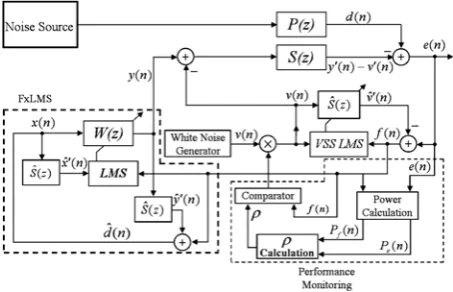
Figure 3 shows block diagram of the proposed ANC system. The residual error signal e(n) of this algorithm is expressed as:
) n ( v ) n ( y ) n ( d ) n (
e = − ′ + ′ y′(n)=s(n)∗y(n), ) n ( v ) n ( s ) n (
v′ = ∗ (5)
Where v(n) is an internally generated white Gaussian noise, which is injected at the output of the control filter W(z).
As we know, Sˆ(z) is the modeling FIR filter with length M that generates vˆ′(n) as expressed below: ) n ( M v ) n ( T sˆ ) n (
As the figure shows, vˆ′(n) generates the error signal for both the modeling filter Sˆ(z) and the control filter W(z) by subtracting from e(n):
) n ( vˆ )] n ( v ) n ( y ) n ( d [ ) n (
f = − ′ + ′ − ′ (7)
Coefficients of the modeling filter Sˆ(z) are updated as follows:
) n ( v ) n ( f ) n ( s ) n ( sˆ ) 1 n (
sˆ + = +μ (8)
Where μs(n) is the step-size parameter of the VSS-LMS algorithm which will be explained later. The output signal yˆ′(n) is used to define estimation of the primary noise dˆ(n):
) n ( yˆ ) n ( f ) n (
dˆ = + ′ (9)
Where x(n)≡dˆ(n) is our reference signal, and )
n (
yˆ′ is expressed as follow:
) n ( M y ) n ( T sˆ ) n (
yˆ′ = (10)
Finally coefficients of the control filter W(z) are updated as below:
) n ( xˆ ) n ( f ) n ( w ) n ( w ) 1 n (
w + = +μ ′ (11)
The input to the LMS algorithm is derived by filtering the reference signal through Sˆ(z):
) n ( M x ) n ( T sˆ ) n (
xˆ′ = (12)
Where xM(n)=[x(n),x(n−1),...,x(n−M+1)]T is an M sample reference signal.
The VSS-LMS algorithm introduced in [3,4] is used to update modeling filter Sˆ(z) coefficients. For more detail on theory of this algorithm reader may refer to [3,4]. As we mentioned before, the modeling filter in Equation 8 is updated using the step-size parameter (μs(n)) of VSS-LMS algorithm and this parameter is calculated using the following three steps [4]:
• Initially, the power of error signals e(n) and f(n) are computed:
) n ( 2 f ) 1 ( ) 1 n ( f P ) n ( f P ) n ( 2 e ) 1 ( ) 1 n ( e P ) n ( e P λ − + − λ = λ − + − λ = (13)
• Then, the ratio of the estimated powers is obtained: 0 ) n ( lim , 1 ) 0 ( ) n ( P / ) n ( P ) n ( n e f → ρ ≈ ρ = ρ ∞ → (14)
• Finally, the step size is calculated as follows:
max s )) n ( 1 ( min s ) n ( ) n (
s =ρ μ + −ρ μ
μ (15)
Where max s , min s μ
μ and λ are the experimentally
Figure 2. Block diagram of feedback ANC system using
FxLMS algorithm. x(n) represents the reference signal.
Figure 3. Block diagram of the proposed feedback ANC
determined values. These values are selected so that the adaptation is neither too slow nor it becomes unstable.
The VSS-LMS algorithm is initially set to a small step size. During the process of this algorithm, μs is increased when the error signal e(n) decreased and vice versa. It needs to be noted that any increase of the step size corresponds to a faster convergence of the adaptive algorithm. Consequently, once W(z) is slow in reducing e(n), the step size remains small which results in a lower convergence rate.
Injection of additional random noise into the ANC system in modeling the secondary path causes instability problem especially in feedback structure. To prevent this problem, the injection of White noise is required to be stopped at the optimum point, which is measured using:
5 . 0 1 . 0 , ) n ( f. ) n
( <α ≤α≤
ρ (16)
At this point, Sˆ(z) converges to a good estimation of S(z). As can be seen from Figure 3, this condition validity is monitored at the performance monitoring stage.
Here, the VSS-LMS algorithm is briefly described to show the way the optimum point is obtained. During the process of this algorithm, μs is increased as the error signal f(n) decreases and vice versa. Hence, the modeling filter, Sˆ(z), converges to a good estimation when f(n) decreases and μs increases as high as
max s
μ . This
happens when ρ(n)→0. Therefore, because both f(n) and ρ(n) decreases down into zero the optimum point defined based on these two signals. As can be seen in Figure 3, this condition validity is monitored at the comparator stage.
In some practical cases the secondary path may suddenly change. This event derives the system to diverge. To prevent such effects, Sˆ(z) needs to be updated. Existing online secondary path modeling techniques [2-7] control the secondary path changes during system operation by continuous injection of the white noise. As described before, in the proposed method injection of the white noise is stopped at the optimum point. To adapt the system with the secondary path changes, the proposed algorithm is designed in such a way that
it can monitor the secondary path variations by the following expression:
0 ) n ( f 10 log
20 < . (17)
If the validity of the above equation is not satisfactory, the system reactivates the VSS-LMS algorithm and injects the white noise to remodel
) z (
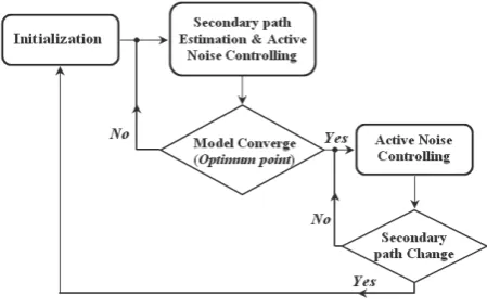
Sˆ . The same as before, the injection is stopped at the optimum point using (17). The above procedure is repeated during the system operation to adapt the algorithm with characteristics of the environment. Figure 4 simply shows procedure of the proposed algorithm.
It is important to note that, all of the primary values of the estimated powers in (13) are set to 1 at the initialization step.
It must be mentioned that, there is no need for using offline estimation of the secondary path in the proposed approach as it is required in the existing methods [3,4,8].
As mentioned before, the proposed method prevents the instability problem raised by white noise injection in the feedback ANC systems. Here we describe the ideal situation of the feedback ANC system and finally explain the instability problem and the proposed method advantage. As Figure 3 shows, the error signal can be expressed as below:
) z ( X ). z ( W ). z ( S ) z ( D ) z (
E = − (18)
The ideal situation of an ANC system happens
when the modeling filter converge which means )
z ( S ) z (
Sˆ ≅ and X(z)≅D(z). By considering this situation Equation 18 updated as follows:
)) z ( W ). z ( S 1 )( z ( D ) z (
E = − (19)
As we know for perfect cancellation, the error signal should become zero, which requires the adaptive filter to converge to the optimum transfer function expressed as:
) z ( S
1 ) z (
Wo = (20)
Therefore, the adaptive filter inversely models the secondary path S(z). As can be seen the behavior and performance of the ANC system is mainly determined by S(z), which is the target for optimization in this paper. Equation 20 shows that the ANC system is unstable if there is a frequency w0 such that S(w0) = 0. This may happen during the secondary path modeling. Therefore stopping the modeling filter after reaching a good estimation makes the FxLMS algorithm work properly for all frequencies.
4. SIMULATIONS and PERFORMANCE RESULTS
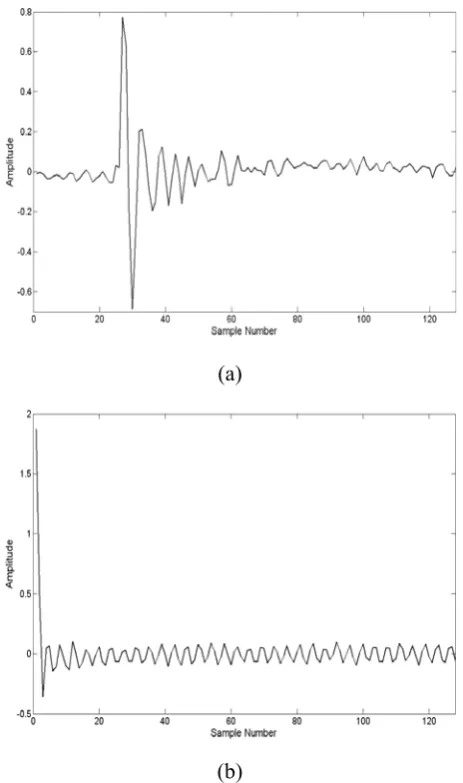
In this section the proposed ANC system is simulated using Matlab version 7.1. In this simulation, the primary path P(z) and secondary path S(z) have been practically extracted using a headphone. The impulse responses of the primary and secondary paths are shown in Figure 5. These paths, P(z) and S(z) are modeled by FIR filters with 128 and 65 tap-weight length respectively. The rate of the sampling frequency in this simulation was 8KHz. Extensive experiments have been performed to find suitable values for a fast and stable performance of the ANC system. Length of the filter Sˆ(z) for modeling the secondary path and length of the adaptive filter W(z) used for the noise cancellation have been chosen 65 (M) and 256 (L), respectively. Due to the limitation of implementing the hardware these values are selected as low as possible.
As mentioned before, the ANC system parameters are selected experimentally but under some certain conditions. The step size of the controller filter W(z) usually is determined by considering the controller filter length (L) and power of the xˆ′ as follows:
L . xˆ P
1 w 0
′ < μ
< (21)
The modeling filter step size μs is calculated using Equation 15 with two constant
min s
μ and max s μ . (a)
(b)
Figure 5. Impulse response of the acoustic paths for the
TABLE 1. Simulation Parameters for the Proposed Approach.
Parameters Description Value w
μ Step-Size for W(Z) 1 × 10⁻⁴
min s
μ Minimum Step-Size for Sˆ(z) 75 × 10-4
max s
μ Maximum Step-Size for Sˆ(z) 24 × 10-3
α Threshold Value in Equation 16 0.3
λ Coefficient in Equation 13 0.99
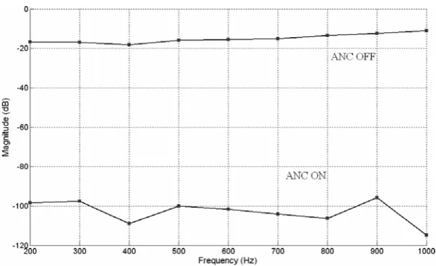
Figure 6. Noise cancellation levels for sinusoidal noise at different frequencies. The top line and
bottom line represent the original noise and residual noise at the error sensor, respectively. These two constant values are defined under the
following criteria:
M . v P
1 s
0 < μ < (22)
The forgetting factor λ which has been used in Equation 13 is limited as below:
1 9 .
0 <λ< (23)
The resulted simulation parameters are summarized in Table 1.
Five experiments using different noises have been performed on the proposed system to evaluate performance of the system. In this evaluation, a
white noise with variance of 0.05 has been used as training signal in secondary path modeling. In the first experiment, a sinusoidal noise in 0.2-1 kHz range and 100 Hz step was used. Figure 6 shows the noise cancellation results in this experiment. As can be seen from the figure, the difference between the noise energy at the error sensor for ANC, OFF and ON is more than 80-dB.
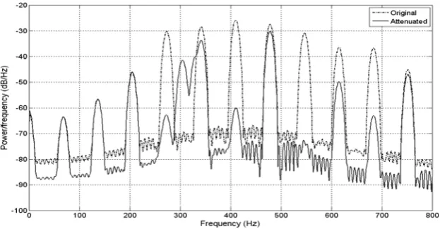
Figure 7. Power spectra for the original engine noise at 2200 rpm (dotted line) and the residual noise (solid line) after noise cancellation.
Figure 8. Power spectra for the original engine noise at 3700 rpm (dotted line) and
the residual noise (solid line) after noise cancellation.
Figure 9. Power spectra for the original engine noise at 4100 rpm (dotted line) and
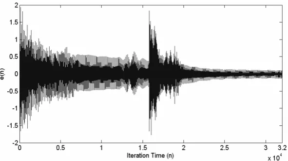
Figure 10. Residual noise signal e(n) of engine noise at 2200 rpm versus iteration time n.
engine noise, and the solid line depicts the residual noise obtained after cancellation.
For engine noise at 2200 rpm, from Figure 7, the noise cancellation levels obtained for harmonic components at 220, 257, 293 and 332 Hz are 44.91, 48.38, 43.56 and 8.48 dB, respectively. Figure 8 shows the results for another engine noise at 3700 rpm. In this figure, the noise cancellation levels for harmonic components at 308, 370, 431, 493 and 617 Hz are 28.71, 35.33, 40.44, 35.75 and 31.38 dB, respectively.
As can be seen from Figure 9, the noise cancellation levels for harmonic components at 273, 410, 547, 615 and 685 Hz for engine noise 4100 rpm are 32.69, 34.19, 42.4, 13.34 and 26.3 dB, respectively.
To show the relationship between the number of iterations and the system accuracy, we plotted the residual noise e(n) of the engine noise at 2200 rpm in Figure 10.
The high noise cancellation results in these experiments indicate the accuracy of the proposed system. In fact, the good modeling of the secondary path has yielded this accuracy. It should be noted that a wrong selection of α in Equation 16 may lead to an inefficient model for Sˆ(z) which drives the system to an instable situation. Figure 11 shows an instable situation of the system’s output. We compared the estimated secondary path
) z (
Sˆ and the original secondary path s(z) in
Figure 12 with the estimation at the optimum point for the engine noise at 3700 rpm. This figure indicates that the proposed algorithm could properly estimate the secondary path.
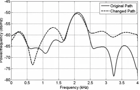
In the last experiment, to show the ability of the proposed method in maintaining its performance against the secondary path changes we assume that the secondary path suddenly changed during the system process. Figure 13 shows the magnitude response of the original and changed path. In this figure, the solid line represents the secondary path at start point, n = 0, and the dashed line represents the changed path at iteration n = 16000. Here we consider the 4100 rpm engine noise as reference signal. The proposed method evaluated on the basis of the residual noise and the MSE in Figures 14 and 15 respectively.
5. CONCLUSION
Figure 11. Output of the proposed system for a non-optimal point α (an instable situation).
Figure 12. Comparing the estimated (solid line) and original secondary paths (dotted line).
Figure 13. Magnitude response of secondary path. (Solid line:
online using White noise as a training signal. The common instability problem of feedback structures was resolved in this research by stopping the White noise injection at the optimum point. The VSS, LMS, algorithm were used in secondary path estimation, which provides an efficient convergence rate. As another advantage of the proposed method, there is no need to use the offline estimation of the secondary path, as it is required in the existing methods.
6. REFERENCES
1. Kuo, S. M. and Morgan, D. R., “Active Noise Control:
A Tutorial Review”, Proc. IEEE, Vol. 8, No. 6, (January 1999), 943-973.
2. Bao, C., Sas, P. and Van Brussel, H., “Comparison of Two Online Identification Algorithms for Active Noise Control”, Pmc. Recent Advances in Active Control of Sound Vibration, (1993), 38-51.
3. Akhtar, M. T., Abe, M. and Kawamata, M., “Modified-Filtered-x LMS Algorithm Based Active Noise Control System with Improved Online Secondarypath Modeling”, Proc. IEEE 2004 Intern. Mid. Symp. Circuits Systems (MWSCAS 2004), Hiroshima, Japan, (2004), 13-16. 4. Akhtar, M. T., Abe, M. and Kawamata, M., “A Method
for Online Secondary Path Modeling in Active Noise Control Systems”, Proc. IEEE 2005 Intern. Mid. Symp. Circuits Systems (ISCAS 2005), (May 23-26, 2005), 264-267.
5. Kuo, S. M. and Vijayan, D., “A Secondary Path Modeling Technique for Active Noise Control Systems”, IEEE Trans. on Speech and Audio Processing, Vol. 5,
Figure 14. Residual error signal.
No. 4, (July 1997), 374-377.
6. Kuo, S. M. and Vijayan, D., “Optimized Secondary Path Modeling Technique for Active Noise Control Systems”, Proc. IEEE Asia-Pacific Conf. on Circuits and Systems, Taipei, Taiwan, Vol. 8C, No. 3. (December 1994), 1-6.
7. Hu, A. Q., Hu, X. and Cheng, S., “A Robust Secondary Path Modeling Technique for Narrowband Active Noise Control Systems”, Proc. IEEE Conf. on Neural Networks and Signal Processing, Vol. 1, (December 2003), 818-821.
8. Gan, W. S., Mitra, S. and Kuo, S. M., “Adaptive Feedback Active Noise Control Headsets: Implementation, Evaluation and its Extensions”, IEEE Trans. on Consumer Electronics, Vol. 5, No. 3, (August 2005), 975-982.
9. Gan, W. S. and Kuo, S. M., “Integrated Active Noise
Control-Communication Headsets”, Proc. IEEE International Symposium on Circuits and Systems, (May 2003), 353-356.
10. Kuo, S. M., Kong, X. and Gan, W. S., “Applications of Adaptive Feedback Active Noise Control System”, IEEE Trans. Contr. Syst. Technol., Vol. 11, No. 2, (2003), 216-220.
11. Gan, W. S. and Kuo, S. M., “Integrated Active Noise Control Communication Headset”, Proc. of International Symposium on Circuits and Systems, (May 25-28, 2003), 353-356.
12. Kuo, S. M. and Panahi, I., “Design of Active noise Control Systems with the TMS320 family”, Texas Instruments, (1996).