A CURRENT-BASED OUTPUT FEEDBACK SLIDING MODE
CONTROL FOR SPEED SENSORLESS INDUCTION MACHINE
DRIVE USING ADAPTIVE SLIDING MODE FLUX OBSERVER
G. R. Arab Markadeh and J. Soltani*
Department of Electrical and Computer Engineering, Isfahan University of Technology Isfahan, Iran, [email protected] - [email protected]
*Corresponding Author
(Received: January 26, 2004 - Accepted in Revised Form: June 1, 2006)
Abstract This paper presents a new adaptive Sliding-Mode flux observer for speed sensorless and rotor flux control of phase induction motor (IM) drives. The motor drive is supplied by a three-level space vector modulation (SVM) inverter. Considering the three-phase IM Equations in a stator stationary two axis reference frame, using the partial feedback linearization control and Sliding-Mode (SM) control, the rotor speed and rotor flux controllers are derived first. These controllers are capable of making the drive system states follow the system nominal trajectories in spite of the motor parameter uncertainties and external load torque disturbance. Then, based on the Lyapunov theory, a SM observer is developed in order to estimate the rotor flux, rotor speed and rotor resistance simultaneously. In addition, in order to satisfy the persistent excitation (P.E) condition, a low frequency low amplitude ac signal is superimposed to the rotor flux reference command. Finally, the validity and effectiveness of proposed control approach is verified by computer simulation.
Key Words Induction Machine, Sliding Mode Control, Adaptive, Output Feedback, Sliding Mode Observer, Speed Sensorless
ﭼ
ﺪﻴﻜ
ﻩ
ﺭﻮـﺗﻮﻣﺭﻮـﺗﻭﺭﻲﺴﻴﻃﺎﻨﻐﻣﺭﺎﺷﻭﺖﻋﺮﺳﻝﺮﺘﻨﻛﻱﺍﺮﺑﺭﺎﺷﻲﺷﺰﻐﻟﺪﻣﺪﻳﺪﺟﺮﮔﻩﺪﻫﺎﺸﻣﻚﻳﻪﻟﺎﻘﻣﻦﻳﺍﻪﻳﺍﺭﺍﻲﻳﺎﻘﻟﺍﺯﺎﻓﻪﺳﻮﻳﺍﺭﺩ ﻲﻣ
ﺪﻨﻛ
.
ﻮﻣ
ﻱﺎﻫﺭﺍﺩﺮﺑﻲﻳﺎﻀﻓﻥﻮﻴﺳﻻﻭﺪﻣﻉﻮﻧﺯﺍﻲﺤﻄﺳﻪﺳﺮﺗﺭﻮﻨﻳﺍﻚﻳﻂﺳﻮﺗﻮﻳﺍﺭﺩﺭﻮﺗ
ﻪﻳﺬﻐﺗﺭﻮﺗﺎﺘﺳﺍﻱﺎﻫﮊﺎﺘﻟﻭﻲﻳﺎﻀﻓ ﻲﻣ
ﺩﺩﺮﮔ
.
ﺎﺑ
ﺭﻮﺗﻮﻣﺕﻻﺩﺎﻌﻣﻦﺘﻓﺮﮔﺮﻈﻧﺭﺩ
ﻭﺩﺕﺎﺼـﺘﺨﻣﻚـﻳﺭﺩﺯﺎـﻓﻪـﺳﻲﻳﺎﻘﻟﺍ
ﻲـﺷﺰﻐﻟﺪـﻣﻝﺮﺘﻨﻛﻭﻲﺟﻭﺮﺧﻱﺩﻭﺭﻭﻱﺯﺎﺳﻲﻄﺧﻝﺮﺘﻨﻛﻱﺎﻬﺷﻭﺭﻱﺮﻴﮔﺭﺎﻜﺑﺎﺑﻭﺭﻮﺗﺎﺘﺳﺍﻦﻛﺎﺳﻱﺭﻮﺤﻣ ،
ﺍﺪـﺘﺑﺍ
ﻛ
ﺝﺍﺮﺨﺘﺳﺍﺭﻮﺗﻭﺭﺭﺎﺷﻭﺭﻮﺗﻭﺭﺖﻋﺮﺳﻱﺎﻫﻩﺪﻨﻨﻛﻝﺮﺘﻨ ﻲﻣ
ﺪﻧﺩﺮﮔ
.
ﺎﻫﻩﺪﻨﻨﻛﻝﺮﺘﻨﻛﻦﻳﺍ ﺎﻗ
ﺮﻴﺴـﻣﺐﻴﻘﻌﺗﻝﺮﺘﻨﻛﺖﻴﻠﺑ
ﺍﺭﺭﻮﺗﻮﻣﻲﻣﺎﻧﻱﺎﻬﺘﻟﺎﺣ
ﺎﻧﺩﻮﺟﻭﻢﻏﺮﻴﻠﻋ ﻲﻨﻴﻌﻣ
ﺎﻫ
ﺎﻫﺮﺘﻣﺍﺭﺎﭘﺭﺩ ﻭﺎﺘﺸﮔﺵﺎﺸﺘﻏﺍﺰﻴﻧﻭ
ﺭﺎﺑﺭ ﺭﺍﺩ ﺍ ﻲﻣ ﺪﻨـﺷﺎﺑ
. ﺮـﺑﻩﺎـﮕﻧﺁ
ﭘ
،ﻑﻮﻧﺎﭘﺎﻴﻟﻱﺭﻮﺌﺗﻪﻳﺎ
ﻪﻌﺳﻮﺗﻲﺷﺰﻐﻟﺪﻣﺮﮔﻩﺪﻫﺎﺸﻣﻚﻳ ﻣ
ﻲ
ﺪﺑﺎﻳ ﺭﺎﺷﻪﻛ ،
ﻘﻣﻭﺖﻋﺮﺳ
ﻦﻴـﻤﺨﺗﺍﺭﺭﻮﺗﻭﺭﺖﻣﻭﺎ ﻲـﻣ
ﺪﻧﺯ
.
،ﻡﻭﺍﺪﻣﻚﻳﺮﺤﺗﻁﺮﺷﻱﺭﺍﺮﻗﺮﺑﺭﻮﻈﻨﻤﺑﻩﻭﻼﻌﺑ
ﻝﺎﻨﮕﻴﺳﻚﻳ
ac
ﻊـﺟﺮﻣﺭﺎـﺷﻝﺎﻨﮕﻴﺳﻪﺑﻢﻛﺲﻧﺎﻛﺮﻓﻭﻪﻨﻣﺍﺩﺎﺑ
ﻪﻓﺎﺿﺍﺭﻮﺗﻭﺭ ﻲﻣ
ﺩﺩﺮﮔ
.
،ﻥﺎﻳﺎﭘﺭﺩ
ﻩﺩﺍﺩﺡﺮـﺷﻱﺮﺗﻮﻴﭙﻣﺎﻛﻱﺯﺎﺳﻪﻴﺒﺷﺎﺑﻱﺩﺎﻬﻨﺸﻴﭘﻝﺮﺘﻨﻛﺵﻭﺭﻥﺩﻮﺑﺮﺛﻮﻣﻭﻱﺭﺍﺮﻗﺮﺑ
ﺩﻮﺷﻲﻣ
.
1. INTRODUCTION
SM theory is one of the prospective control methodologies for IM flux and speed control because of its order reduction, disturbance rejection, strong robustness and particularly its simplicity of implementation by power converters [1,2]. SM observers have also robust features as SM controllers. So far, a few research reports have been reported for the speed and rotor flux estimation of the IM using an SM observer [3,4].
proposed for choosing the gains of the adaptive flux observer.
A closed loop current model SM flux observer has been proposed in [5] and used to estimate the rotor speed, rotor position and rotor flux vector components of a 5kW cage rotor IM in a fixed stator α−β: axis reference frame. The rotor flux observer of [5] has two main drawbacks: First is that with constant rotor flux amplitude, it is not possible to detect the correct values of rotor time constant and rotor speed simultaneously [6,7].This is due to the fact that we can not separate the speed and rotor time constant estimated errors from the stator variables in a steady state. Second is that, according to the equivalent control concept described in [5], the estimation of error of the speed and rotor time constant will only converge to zero if the stator currents and the rotor flux estimated errors also tend to zero. Therefore in transient conditions especially in the reaching phase condition of SM flux observer, the indirect-field orientation (IFO) control of the IM drive system may lost.
To overcome the above problems, this paper presents the following research:
1. Considering the IM Equations in a α−β: axis stationary reference frame, using the partial feedback linearization control, two input-output state variables are introduced and used to decouple the dynamics of IM torque and rotor flux magnitude.
2. By combining the SM control and Linear Quadratic (LQ) feedback control method, the composite rotor speed and rotor flux controllers are derived and create the merits for easy design, simplicity of implementation by power electronic devices, strong robustness with minimum chattering and no reaching phase.
3. A closed loop current model SM rotor flux observer is derived in order to provide the simultaneous estimation of rotor speed, rotor time constant and rotor flux vector components in a stator fixed two axis reference frame. The stability of the SM observer is proved by the Lyapanuv theory. In addition, in order to satisfying the P.E condition and convergent behavior of the SM observer, a low frequency low amplitude ac signal is superimposed to the rotor flux reference command [8].
4. A three-level SV-based PWM inverter is
employed to feed the induction drive system. A so- called vector classification algorithm based on Artificial Neural Network (ANN), is applied to obtain the PWM inverter switching patterns and on-duration of power electronic devices [11]. This method reduces software and hardware complexity, decreases the computation time and increases the accuracy of the positioning switching instants.
2. SYSTEM DYNAMIC EQUATIONS
The fifth order model of the three-phase induction machines in a stationary α−β: axis reference frame with stator currents, rotor speed and rotor flux as variables are defined by:
s v 01 B r s i 22 A 21 A 12 A 11 A r s i t d d ⎥ ⎦ ⎤ ⎢ ⎣ ⎡ + ⎥ ⎥ ⎦ ⎤ ⎢ ⎢ ⎣ ⎡ φ ⎥ ⎥ ⎦ ⎤ ⎢ ⎢ ⎣ ⎡ = ⎥ ⎥ ⎦ ⎤ ⎢ ⎢ ⎣ ⎡
φ (1)
m J l T J T s i μ m ω m J f B m ω dt
d =− + φ− (2)
With ⎥ ⎥ ⎦ ⎤ ⎢ ⎢ ⎣ ⎡ = s q i s d i s i , ⎥ ⎥ ⎥ ⎦ ⎤ ⎢ ⎢ ⎢ ⎣ ⎡ ϕ φ = φ s r q s r d
r ⎥⎥
⎦ ⎤ ⎢ ⎢ ⎣ ⎡ = s q v s d v s v I α M β σ s R 11
A ⎟⎟
⎠ ⎞ ⎜ ⎜ ⎝ ⎛ + −
= , A21=Mαα
⎟ ⎠ ⎞ ⎜ ⎝ ⎛ − =β αI ωrJ 12
A , A22=−αI+ωrJ
σ I 1
B = , ⎥
⎦ ⎤ ⎢ ⎣ ⎡ = 1 0 0 1
I , ⎥
⎦ ⎤ ⎢ ⎣ ⎡ − = 0 1 1 0 J r L r R
α = ,
⎟⎟ ⎟ ⎠ ⎞ ⎜⎜ ⎜ ⎝ ⎛ − = r L s L 2 m L 1 s L σ r L m J m L
μ = ,
r
σLm
L
β =
s
R and Rr: stator and rotor resistance
s
L and Lr: stator and rotor inductance
m
L : mutual inductance σ: leakage coefficient
α: reverse of the rotor time constant m
ω : rotor mechanical angular speed
r
ω : rotor electrical angular speed
m
J : moment of inertia
f
B : friction coefficient
Using Equations 1 and 2, based on partial feedback linearization control, the following control inputs are introduced.
⎥ ⎥ ⎦ ⎤ ⎢ ⎢ ⎣ ⎡ = ⎥ ⎥ ⎦ ⎤ ⎢ ⎢ ⎣ ⎡ φ
s q i
s d i T T U U
(3)
with
⎥ ⎥ ⎦ ⎤ ⎢
⎢ ⎣ ⎡
φ Φ φ Φ −
φ φ
Φ =
r d r r q r
r q r
d r 1 T
Linking Equations 1-3, yields
m Jl
T T U m JT K m m J
B m dt
d ω =− ω + − (4)
Φ τ + Φ τ − =
Φ U
r m L r r 1 r dt
d (5)
where
r Lm L 4
P 3 T
K = and P is number of stator poles.
From Equations 4 and 5, the feedback-state variables UTand UΦ, can be used to control the rotor speed and rotor flux independently. However, in the perturbed condition, while the parameter uncertainties and the disturbance load torque occur, it is necessary to decouple the rotor flux dynamic from the rotor speed dynamic completely.
The way of doing that is explained in the subsequent section.
3. SLIDING-MODE CONTROLLER
A. Purpose of Design
In this section, based onstate-space Equations of the linear system and the introduced performance index, the general control concepts of the LQ feed back control is used to design a linear control to satisfy the IM dynamic system requirements. The pole placement method is an adequate way to meet this objection, if an optimal performance index is also considered. The LQ feed back control method is easily able to determine the desired feed back gains to satisfy the requirements, however the method will not be able to conserve the responses as the nominal condition once parameter uncertainty and external load torque disturbance are present. in order to conserve the responses and reject the effects of the external disturbance and parameters uncertainties, the system controllers are designed by combining the classical LQ feed back control and SM control. Using these composite controllers, it will be shown that the rotor speed and rotor flux controllers are insensitive to uncertainties and external unknown load torque.
B. Nominal System Control
The stateEquations 4 and 5 in matrix form become l
T . d ) t ( bU Ax
x& = + + (6)
where
⎥ ⎥ ⎦ ⎤ ⎢
⎢ ⎣ ⎡
− − =
Φ a ω a 0
0
A ,
⎥ ⎥ ⎦ ⎤ ⎢
⎢ ⎣ ⎡
Φ ω =
b 0
0 b
b ,
⎥ ⎥ ⎦ ⎤ ⎢ ⎢ ⎣ ⎡
Φ =
UT
U U
and
m J
B = ω
a ,
m J
T K
bω= ,
m J
1 d= −
r 1 τ = φ
a ,
r m L b
τ = Φ
can be derived as: ) t ( f ) t ( bU Ae
e= + +
& (7)
where
T e w e
e=⎢⎣⎡ φ⎥⎦⎤ , eω=ωrm−ωref Φ
− Φ =
φ r ref e
and
⎥ ⎥ ⎦ ⎤ ⎢ ⎢ ⎣ ⎡ = ⎥ ⎥ ⎦ ⎤ ⎢
⎢ ⎣ ⎡
φ +
+ +
−
= (t)
Φ f
(t) ω f
ref Φ ref Φ
l d.T ref ω ω ref ω (t) f
a a
& &
In view of the LQ optimal control for a double input system described by Equation 7, a performance index J is defined as:
R U T R e
0 eTQ
2 1
J= ∫ ∞ + (8)
where Q and R positive diagonal weighting matrices so that Q=diag(qω,qφ), R=diag(r,r). Via LQ method, to find the optimal control law in an infinite period, the Riccati Equation:
0 P bT R 1 Pb Q PA P
AT + + − − = (9)
must be solved. Thus, the control law to yield a minimum performance index is obtained as:
⎥ ⎥ ⎥
⎦ ⎤
⎢ ⎢ ⎢
⎣ ⎡ = − = −
− =
* Φ U
* T U Ke P)e bT R 1 (
U (10)
In Equation 9 since A, b and R are the diagonal matrices, hence P must also be a diagonal matrix. As a result K has to be a diagonal matrix too.
⎥⎦ ⎤ ⎢⎣
⎡
=diag Kω,Kφ
K (11)
C. Perturbed System Control
ConsiderEquation 7 with uncertainties so that
r(t) bU Ae
e= + +
& (12)
where
= ⎥ ⎥ ⎦ ⎤ ⎢ ⎢ ⎣ ⎡ =
φ r rω r(t)
⎥ ⎥ ⎦ ⎤ ⎢
⎢ ⎣ ⎡
φ + φ φ +
+ +
φ
U b Δ e α Δ Φ
f T
U ω b Δ ω e ω a Δ ω f
(13)
In fact ΔA and Δb are denoted as the uncertainties introduced by system parameters,
B ,
J and KT.r(t) called, “lumped uncertainty”. Let the system be under linear state feed back control (U) described by (10), the closed loop dynamic, in the nominal condition, is verified by
e C A e ) bK A (
e&= − = `(14)
At this stage, the LQ feed back control and SM control are combined in order to design the system control laws capable of reserving an equivalent system dynamic as well as the closed loop dynamic for the perturb system same as the nominal condition.
The SM control objective consists of designing First equilibrium surfaces S(e,t)∈R2, such that the state trajectories of the plant restricted to the equilibrium surfaces have a desired behavior in terms of tracking, relation and stability. Secondly, according to the SM reaching condition, the switching control effort Uc(e,t) is determined so as to be able to curb the state trajectories to the equilibrium surfaces and maintain them on the surfaces so that eω and eφ (the rotor speed and rotor flux amplitude errors) converge to zero as well as reserve the system trajectories as the nominal condition.
In the classical SM control, the chattering is a bothering problem. To reduce this effect, the SM speed and rotor flux controllers are derived based on using the switching surfaces with integral components, which posses the exponential stability [17].
dτ t
0 (ττ e c A T C e(0)] e(t) T [C Φ
Sω
S
S = − − ∫
⎥ ⎥ ⎦ ⎤ ⎢ ⎢ ⎣ ⎡
= (15)
where Ac = A −bKT and cT are (2*2) positive diagonal matrix and e(0) is the initial state of vector e(t).
diagonal matrices.
Consider Equation 13, under the nominal condition. It is due to the state feedback given by Equation 10, that the system control posses the sliding surfaces S(e,t)=0 on which the states slide. In addition, since S(0)=0 at t=0, there is no reaching phase as in the conventional SM control. Under the influence of uncertainty and disturbance, the perturbed and uncertain system cannot still preserve the system response as the nominal condition; and the system performance under the control of Equation 10, which is designed for the nominal system, is surely degraded. Moreover the minimum performance index cannot be achieved and the sliding condition cannot be maintained either.
To maintain the sliding condition and preserve the nominal system response and performance subjected to the uncertainty and/or external disturbance, additional control effort is required in order to ensure the SM reaching conditions that are described by
0 F
F&< (16)
where F= diag(Sω,SΦ).
To control the states on the sliding surfaces under the system perturbed condition, an extra control effort must be chosen as:
ρsgn(S)
c
U =− (17)
Then the total system control is:
⎥ ⎥ ⎥
⎦ ⎤
⎢ ⎢ ⎢
⎣ ⎡ = −
− = + =
* Φ U
* T U ) S (
ρsgn
e T K L U C U
U (18)
where ρ=diag[ρω,ρΦ].
The added term, −ρsgn(S) , is the variable structure control for the system and S is the sliding switching functions described by Equation 15. Linking Equations 12, 15, 16 and 18, it can be shown that
0 SΦ ]. ) SΦ ( sgn ρΦ bΦ rφ [ ) t ( SΦ ). t ( SΦ
0 Sω ]. ) Sω ( sgn ρω bω rω [ ) t ( Sω ). t ( Sω
≤ −
=
≤ −
=
& &
for t > 0 (19) Combining Equations 13 with 19 yields
max )
eΦ
Φ k Φ Δb Φ e Φ Δa Φ (f ) φ Δb Φ (b
1 Φ
ρ
max )
eω
kω
ω Δb ω e ω Δa ω (f ) ω Δb ω (b
1 ω
ρ
+ +
− >
+ +
− >
(20) Therefore from Equation 20, the lower bands of
ω
ρ and ρΦ can be obtained as
) Φ f Φ e Φ (ε Φ β Φ b
1 Φ
ρ
) ω f ω e ω (ε ω β ω b
1 ω
ρ
+ −
=
+ −
=
(21)
Where
ω β ω
Δb < , Δaω+Δbω kω <εω,
Φ β Φ
Δb < , ΔaΦ +ΔbΦ kΦ < εΦ
and εω,εΦ are positive constants. A consequence the curbing condition F(t)F&(t)<0 is assured. In addition the closed loop system dynamics for the nominal condition can be obtained, i.e. the system will have its activity like e&=Ace regardless of the existence of disturbance and uncertainty. In view of Equation 15, it is evident that S(t)=0 at t = 0 and also later than that. Thus, a system controlled by the proposed rotor speed and rotor flux-controllers is in the sliding-mode at the beginning, i.e. the system can have robust properties from the beginning of the control process.
4. SLIDING-MODE OBSERVER
A. Nonlinear Robust Observer with
Discontinuous
Parameters and stator currents
and voltages as input variables, is proposed so that the rotor speed and rotor time constant can be estimated simultaneously.
⎥ ⎥ ⎦ ⎤ ⎢ ⎢ ⎣ ⎡ − ⎥ ⎥ ⎦ ⎤ ⎢ ⎢ ⎣ ⎡ + ⎥ ⎥ ⎦ ⎤ ⎢ ⎢ ⎣ ⎡ ⎥ ⎥ ⎦ ⎤ ⎢ ⎢ ⎣ ⎡ = ⎥ ⎥ ⎦ ⎤ ⎢ ⎢ ⎣ ⎡ 0 ) s i ~ Ksgn( s v 01 Bˆ r φˆs i 22 Aˆ 21 Aˆ 12 Aˆ 11 Aˆ r φˆs iˆ dt d (22) where I ˆ M s R 11
Aˆ ⎟⎟
⎠ ⎞ ⎜ ⎜ ⎝ ⎛ α β + σ −
= ,
(
ˆI ˆ rJ)
r L M 12
Aˆ α −ω
σ = I ˆ M 21
Aˆ = α , Aˆ22=−αˆI+ωˆrJ
α Δ + α =
αˆ n ˆ ,
⎥ ⎥ ⎦ ⎤ ⎢ ⎢ ⎣ ⎡ = q k 0 0 d k K
where αn is the nominal value of
α
Combining Equations 1 and 18, gives⎥ ⎥ ⎦ ⎤ ⎢ ⎢ ⎣ ⎡ ⎥ ⎥ ⎦ ⎤ ⎢ ⎢ ⎣ ⎡ + ⎥ ⎥ ⎦ ⎤ ⎢ ⎢ ⎣ ⎡ ⎥ ⎥ ⎦ ⎤ ⎢ ⎢ ⎣ ⎡ = ⎥ ⎥ ⎦ ⎤ ⎢ ⎢ ⎣ ⎡ r
φˆs
i
22 A~ 21
A~ 12
A~ 11 A~ r φ ~s i ~ 22 A 0 12 A 0 r φ~ s i ~ dt d ⎥ ⎥ ⎦ ⎤ ⎢ ⎢ ⎣ ⎡ − 0 ) s i ~ (
Ksgn (23)
where s i s iˆ s i ~ = −
, φ~r = φˆr − φr α αˆ α ~ = − , r ω r ωˆ r
ω~ = −
I α ~
βM
11
A~ =− , A~12 = β
(
α~I − ω~rJ)
Iα ~ M 21
A~ = , A~ 22 = −α~I + ω~ rJ
Candidating the following positive definite Lyapunov function ⎟ ⎟ ⎠ ⎞ ⎜ ⎜ ⎝ ⎛ + +
= α~2
α c 1 2 r ω~ ω c 1 r φ ~ T r φ ~ 2 1
V (24)
Derivating V with respect to time t, yields
⎟ ⎟ ⎠ ⎞ ⎜ ⎜ ⎝ ⎛ − + −
= ω~r (Jφˆr )Tφ~r ω c 1 m ω~ r φ ~ T r φ ~ α
V& &
(
)
⎟⎟ ⎠ ⎞ ⎜ ⎜ ⎝ ⎛ − −+ α~ φˆ r M iˆs Tφ~r
α c
1 α
~ & (25)
To conserve the observer convergence, it is required to have V& <0. Therefore from Equation 24 r ~ T ) r ˆ J ( c r
~ φ φ
ω =
ω& (26)
(
)
T~rs iˆ M r ˆ c
~ φ − φ
α =
α& (27)
Equations 22 and 23 provide two adaptive laws in order to estimate the rotor speed and rotor time constant simultaneously.
From the IM fifth order model shown in Equation 1, one can show that
⎟ ⎟ ⎠ ⎞ ⎜ ⎜ ⎝ ⎛ − φ =
φ is
σ s β 1
r (28)
Once the estimated error of the stator flux ~φs is
known, then ~φr can be obtained from Equation 27 Using the stator voltage Equation as
s v s i s R
s = − +
φ& (29)
The stator flux vector can be estimated as:
) s i ~ ( sgn K s v s i s R s
ˆ =− + −
φ& (30)
From Equations 26 and 29, the stator flux estimated error is obtained as:
) s i ~ ( sgn K s ~ = −
φ& (31)
Using a first order low pass filter as [5]
s ~ 1 s μ 1 eq s ~ φ + =
φ (32)
where (
μ1 ) the filter low pass cut-off frequency is sufficiently small enough to allow slow component of the motion but is large enough to eliminate the high frequency component. Combining Equations 27 and 31, the rotor flux estimated error is obtained as
⎟ ⎟ ⎟ ⎠ ⎞ ⎜ ⎜ ⎜ ⎝ ⎛ − φ =
φ ~is
σ eq s ~ β 1 r
~ (33)
B. Parameter Convergence
The PE condition implies that if the estimation error dynamic, ~θ, is described as [10]ΓWx θ
~
− =
& (34)
and ∫ +0t TW(τ) WT(τ)dτ is positive definite for some T > 0 and every t > 0, then, the estimation errors will converge exponentially to zero.
From Equations 25 and 26
⎥ ⎦ ⎤ ⎢ ⎣ ⎡ α ω = θ ~~m
~ ,
r ~
x=φ , Γ=diag(cω,cα)
⎥ ⎥ ⎦ ⎤ ⎢ ⎢ ⎣ ⎡ − φ φ = T ) s Mi r ˆ ( T ) r ˆ J (
W (35)
and then
[
Jˆr ˆr Lmis]
T ) s i m L r ˆ ( T ) r ˆ J ( T
WW φ φ −
⎥ ⎥ ⎦ ⎤ ⎢ ⎢ ⎣ ⎡ − φ φ
= (36)
⎥ ⎥ ⎥ ⎦ ⎤ ⎢ ⎢ ⎢ ⎣ ⎡ φ + φ − φ φ − − φ φ − φ φ − − φ φ − φ + − φ = 2 qr ˆ 2 dr ˆ ) qs i m L qr ˆ ( dr ˆ ) ds i m L dr ˆ ( qr ˆ ) qs i m L qr ˆ ( dr ˆ ) ds i m L dr ˆ ( qr ˆ 2 ) qs i m L qr ˆ ( 2 ) ds i m L dr ˆ (
To satisfy the mentioned condition, it is necessary to have Det(WWT)>0.
2 )] qs i m L qr ˆ ( qr ˆ ) ds i m L dr ˆ ( dr ˆ [ ) T WW (
Det = φ φ − +φ φ −
2 ] r ˆ U m L 2 r ˆ [ 2 )] qs i qr ˆ ds i dr ˆ ( m L 2 r ˆ
[Φ − φ +φ = Φ − φΦ
=
(37) Equating 37 to zero, it yields
φ = L m U r
Φˆ (38)
On the other hand, from Equation 5, it can be concluded: Det(WWT)=0. Therefore, in steady
state conditions under the assumption of a constant rotor flux amplitude Det(WWT)=0 and as a result the PE condition is not satisfactory.
Now consider Equation 23 in a steady state condition and with the assumption of (~φ&r =~φr =0)
) r ˆ J .( r ~ ) r ˆ s Mi .(
~ −φ = −ω φ
α (39)
Equation 39 shows that the steady state error exists in the rotor speed and rotor time constant estimations, even if the stator current and rotor flux estimation errors exponentially converge to zero. To solve this problem, the rotor flux reference command has to be contained enough in distinct frequencies in order to satisfy PE conditions. Therefore a low frequency low amplitude ac signal is superimposed to the rotor flux reference signal. In our case, the frequency of this signal is 3Hz and its amplitude is about 4% of the rated rotor flux. One may note that if the aim is only to estimate the rotor speed with tuned rotor resistance (~α=0), in this case the P.E. is always satisfactory and hence no need to use a low frequency, low amplitude ac signal.
In our proposed control method, it is assumed that the rotor resistance and rotor speed are unknown constant parameters; such an assumption is reasonable because the dynamics of rotor speed and rotor resistance are slow enough compared to stator voltages and currents dynamics.
5. SVM INVERTER
Figure 1. Three-level voltage source inverter.
Figure 2. Switching states of Three-level inverter.
high number of devices, (2) the complexity of the controller increases and (3) the balance of the neutral point must be assured.
A. Three-Level Space Vector Modulation
and Switching Instants
As shown in Figure 1,a 3-level voltage source inverter has 27 allowed switching states. The Park transformation of these vectors, project them to a two-layer hexagon center at the origin of the αβ plane and zero voltage vector at the origin of the plane as depicted in Figure 2.
Based on the SVM technique, the reference output voltage is generated by the nearest permitted switching vectors. The active time duration of each switching state is given by the SVM strategy. For example if the tip of reference voltage lie in triangle # 3, we have,
4 t 4 V 3 t 3 V 1 t 1 V s T ref
V = + +
θ
= j
ref Ve
V
2 / E 1
V = , V3=E 3/2.ejπ/6
3 / j e . 2 / E 3
V = π (40)
⎥ ⎥ ⎥
⎦ ⎤
⎢ ⎢ ⎢
⎣ ⎡
θ θ
⎥ ⎥ ⎥ ⎥
⎦ ⎤
⎢ ⎢ ⎢ ⎢
⎣ ⎡
− −
− =
⎥ ⎥ ⎥
⎦ ⎤
⎢ ⎢ ⎢
⎣ ⎡
sin cos 1
s mT s mT 3 s T
s mT s
mT 3 s T
s mT 2 0
s T
4 t3 t1 t
where m is modulation index and described as
E V . 3 2
m = (41)
and Ts is the cycle period, Vref is the reference voltage vector, t1,t2 and t3are the active time duration of the adjacent switching vectors V1,V2 and V3, respectively.
It must be noted that in the Artificial Neural Network implementation of the SVM, nonlinear cosine and sin functions are obtained from a competitive neural network.
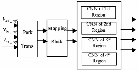
B. Region and sector Detection
Classification algorithm is used to find the number triangle in which the tip of the reference voltage vector lies. This algorithm employs a Classifier Network to distinguish between 4 separate decision areas in one sector (Figure 3).The proposed structure of Figure 4 consists of four different paths; each one is a Classifier Neural Network (CNN) and represents the region of one triangular area. When the tip of the reference voltage vector lies on area, the corresponding path will have a “1” in its output, while all other paths have “0” in their outputs.
Figure 3. First switching sector.
Figure 4. Sector and region detector based on CNN.
Figure 5. CNN for region # 3.
TABLE 1. Neutral Point Current.
Positive Small Vectors NP
i
Negative Small Vectors NPi
MediumVectors
i
NPONN
i
a POO−
i
a PONi
bPPO
i
c OON−
i
c OPNi
aNON
i
b OPO−
i
b NPOi
cOPP
i
a NOO−
i
a NOPi
bNNO
i
c OOP−
i
c ONPi
aPOP
i
b ONO−
i
b PNOi
cexample the detailed structure of the third path is shown in Figure 5. The mapping block in Figure 4, maps all other five sectors to sector # 1, by subtracting appropriate multiples of π/3 to the phase of Vref.
C. Neutral point voltage balancing
Allavailable voltage space vectors for 3-level VSIs are shown in Figure 2. Each phase a, b and c can be connected to either positive (P), negative (N), or neutral (O) points of the DC link. Not all the vectors affect the NP balance. The ones that do are summarized in Table 1 [12]. Large vectors do not affect the NP balance because they connect the phase currents to either the positive or negative DC rail, and the NP remains unaffected. Medium vectors connect one of the phase currents to the
NP, making the NP potential dependent, in part, on the loading conditions. They are the most important sources of the NP potential unbalance. Small vectors come in pairs. Each vector in a pair generates the same line-to-line voltages.
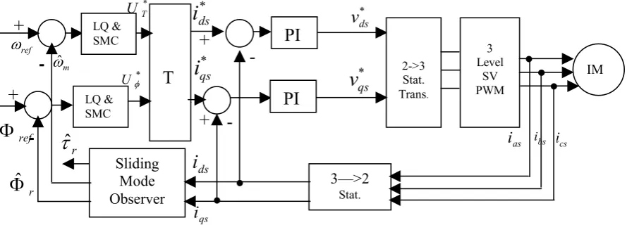
3 Level
SV PWM
Sliding Mode Observer
T
3—>2
Stat.
PI
2->3 Stat. Trans.
IM *
ds
i
*
qs
i
*
φ
U *
T
U
m
ωˆ
r
Φ
ˆ
r
τ
ˆ
ds
i
qs
i
as i ibs
*
qs
v
-+
LQ &SMC
LQ & SMC
cs
i
-ref
Φ
+
+
+
-ref
ω
PI
*
ds
v
Figure 6.Drive system block diagram.
TABLE 2. Motor Parameters.
Power 11 kW f 50 Hz
r
R .371Ω Lm 84.2 mH
s
R .415Ω Lr 87.5 mH
Pole 4 Ls 86.9 mH
f
B .00004 Jm .15 kgm2
to compensate for the error in the NP.
In [12], a good review on neutral point dc control is done and active, passive and hysteresis control methods are compared. Passive control, where the positive and negative small vectors are selected alternatively in each new switching cycle, is suggested for perfectly balanced loads. The hysteresis type control is the simplest method for NP control and requires the knowledge of current direction and then a suitable small vector is selected to compensate NP voltage. At last, the active control is a complicate method and requires measurements of NP voltage and phase currents to control current modulation indexes of small vectors. This method increases the switching losses due to additional switching states.
In our case, we use passive control to neutral point balancing, by a symmetric pattern in each switching period.
The voltage of dc link center tap point is given by [12]:
∫ τ τ
+ =
− 2dc C1 0tiNP( )d V
tap center
V (42)
6. SYSTEM SIMULATION
The block diagram of Figure 6 is proposed for closed loop speed sensorless control of the IM drive system.
A C++ computer program was developed to model the machine drive system. A static Runge-Kutta fourth order method was used to solve the system Equations. The effectiveness of the proposed control approach is verified by computer simulation and is tested with parameters shown in Table 2 for a (11kW, 380V, 50Hz), cage rotor IM by computer simulation. For this motor, the coefficients of SM controllers, SM observer and conventional PI regulators are obtained by trial and error method.
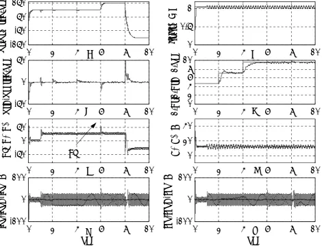
Computer simulation results shown in Figure 7 obtained for an operating condition of ω*r = 100rad/sec. (applied at zero second and stepped up to 150rad/sec at 6sec.), Tl = 73N.m at 1sec.
(Rr=1.5Rrn, at t = 4 sec) and (Rr = 2Rrn, at t = 6
sec.); where
ω
*r is the rotor speed reference, Tl is0
2
4
6
8
10
-150
-50
50
150
wr,
w
r*
(ra
d/
se
c)
sec
0
2
4
6
8
10
-50
0
50
wr
H-wr
(r
ad
/s
ec
)
sec
0
2
4
6
8
10
0
0.5
1
fir,
fir*
(Wb
)
sec
0
2
4
6
8
10
0
2
4
6
8
10
1/
T
r,1
/T
rH
(
1/s
ec
)
sec
0
2
4
6
8
10
-50
0
50
Tl,
uT,
uT
*
sec
0
2
4
6
8
10
0
20
40
uF
,u
F
* (
A
)
sec
0
2
4
6
8
10
-100
0
100
id
s,
id
sH
-id
s (
A
)
sec
0
2
4
6
8
10
-100
0
100
iq
s,
iq
sH
-iq
s (
A
)
sec
Tl
(a)
(b)
(c) (d)
(e) (f)
(g)
(h)
Figure 7. Drive system performance (a) rotor speed (b) estimated rotor flux (c) rotor speed estimation error (d) estimated rotor time constant (e) torque control signal (f) flux control signal (g,h)
stator d and q axis cur.
0 4 8 1 2 1 6
0 2 0 4 0 6 0 8 0 1 0 0
w
r,
w
r*
(
ra
d/
se
c)
0 1 0 2 0
0 0 .5 1 1 .5
fir
,fi
r*
(
W
b)
0 4 8 1 2 1 6
0 5 1 0
1/
T
r,1
/T
rH
(
1/s
ec
)
s ec s e c
Figure 9. Drive performance without an ac signal superimposed to the rotor flux reference command.
0 1 2 3 4
-5 0 5 10 15
wr,
w
r*
(re
d/
se
c)
0 1 2 3 4
0.35 0.4 0.45 0.5 0.55
R
s(
ohm
)
Figure 10. Rotor Speed response with stator resistance misestimating.
(a)
(b) (c)
From these results, one can see that the proposed system control scheme is robust and stable, subject to the motor parameter uncertainties and motor load torque disturbance. In addition, the rotor speed, rotor time constant, stator currents and estimated rotor flux magnitude track their objective reference values.
Some slow oscillations seen on the motor estimated quantities are due to the low-frequency ac signal component that superimposed on the rotor flux reference command ( *
r
φ ) in order to satisfy the P.E conditions. Moreover, from computer results obtained, the decoupling between the torque dynamic and dynamic of the rotor flux magnitude is quite obvious. That is because of the torque and rotor flux control states (UT,Uφ),
which perfectly track their respected reference signals ( *
T
U ,U*φ). Moreover, the drive system
performance in the low speed region can be seen in Figure 8. These results are obtained for ( *
r ω = 10rad/sec, applied to zero sec, stepped down to zero at 8sec and stepped up to 100rad/sec at 10sec.) for (Rr = 1.5Rrn, at t = 4 ec.), (Rr = 2Rrn, at t = 6 sec.) and (B=3Bn,J=3Jn, at 10sec.) Figure 9 shows that for constant rotor flux amplitude, the PE conditions a are not satisfied. As a result the steady-state error is expected in the rotor speed and rotor time constant estimations. Furthermore the stator resistance variation affects the performance in the IM low speed operating region is as shown especially in Figure 10.
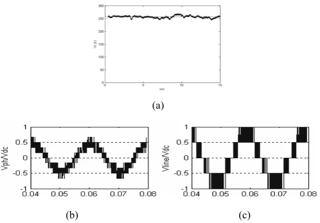
Finally, simulation results obtained corresponding to three-level SV-based PWM inverter are given in Figure 11.
7. CONCLUSIONS
Based on partial feedback linearization control, using the induction machine Equations in a stator
β −
α : fixed axis reference frame, the dynamics of the IM torque and rotor flux modulus have been decoupled first.
Combining SM control and LQ feedback control methods, the composite speed and rotor
flux controllers have been derived to make the IM states follow their nominal trajectory as obtained by the LQ controllers. An SM rotor flux observer has been developed in order to provide the estimation of rotor speed, rotor time constant and the α−β: axis rotor flux components simultaneously. The stability of this observer is proved by Lyapunov stability theory. A three-level SV-based PWM inverter has been employed that feeds the IM drive system. This inverter compared to conventional two-level PWM inverter, has a better utilization of the dc link voltage with less torque pulsation assuming the same switching frequency.
A low frequency, low amplitude ac signal is superimposed to rotor flux reference command, in order to satisfy the persistency of excitation condition.
Computer simulation results obtained have shown the validation of the proposed control approach. However these results have shown that for further improvement of the IM drive system robustness, especially in low speed operating regions, it is also required to estimate the stator resistance parameter. This needs more research which is out of the scope of the present paper.
8. REFERENCES
1. Do Ki, S., Sangwonwnich, S., et al., “Implementation of speed-sensorless field oriented vector control using adaptive sliding observers”, in Proc. IEEE IECON’92, (1992), 453-458.
2. Utkin, V. I., “Sliding mode control design principles and applications to electric drives”, IEEE Trans. Ind. Elect., Vol. 40, No. 1, (Feb. 1993), 23-36.
3. Benchaib, A., Rachid, A., Audrezet, E. and Tadjine, M., “Real-time sliding-mode observer and control of an induction motor”, IEEE Trans. Ind. Appl., Vol. 46, No.
1, (Feb. 1999), 128-138.
4. Tursini, M., Peralla R. and Parasiliti, F.,“Adaptive sliding mode observer for speed-sensorless control of induction motors”, IEEE Trans. Ind. Appl., Vol. 36,
No. 5, (Sept. 2000), 128-137.
5. derdiyok, A., Guven, M., Rahman, H., Inanc, N., Xu, L., “Design and implementation of a new sliding-mode observer for speed-sensorless control of induction machine”, IEEE Trans. Ind. Elect., Vol. 49, No. 5,
(Oct. 2002), 1177-1182.
(Sep.-Oct. 1994), 1219-1224.
7. Tajima, H., Guidi, G. and Umida, H., “Consideration about problems and solutions of speed estimation method and parameter tuning for speed-sensorless vector control of induction motor drives”, IEEE Trans. Ind. Appl., Vol. 38, No. 5, (Sep.-Oct. 2002), 1282-1289.
8. Mondal, S. K., Pinto, J. and Bose, B. K., “A neural-network-based space-vector PWM controller for a three-level voltage-fed inverter induction motor drive”, IEEETrans. Ind. Appl., Vol. 38, No. 3,
(May-June 2002).
9. Wai, R. J., “Adaptive sliding–mode control for induction servo motor drive”, IEE Proc. Electr. Power.
Appl., Vol. 147, No. 6, (Nov. 2000), 553-562.
10. Marino, R. and Tomei, P., Nonlinear Control Design-Geometric, Adaptive and Robust. Englewood Cliff, VJ: Prentice-Hall, (1995).
11. Bakhshai, A. R., Saligheh Rad, H. R. and Joos, G., “Space vector Based on classification method in three-phase multi-level voltage source inverters”, IEEE Proc., (2001), 597-602.
12. Celanovic, N. and Boroyovich, D., “A comprehensive study of neutral-point voltage balancing problem in the three-level neutral-point-clamped voltage source PWM inverters”, IEEE Trans. on Power Electr., Vol. 15, No.