https://doi.org/10.5194/gmd-10-4081-2017 © Author(s) 2017. This work is distributed under the Creative Commons Attribution 3.0 License.
Implementation of methane cycling for deep-time global warming
simulations with the DCESS Earth system model (version 1.2)
Gary Shaffer1,2, Esteban Fernández Villanueva3, Roberto Rondanelli3,4, Jens Olaf Pepke Pedersen5, Steffen Malskær Olsen6, and Matthew Huber7,8
1GAIA-Antarctica, Universidad de Magallanes, Punta Arenas, Chile
2Niels Bohr Institute, University of Copenhagen, 2100 Copenhagen Ø, Denmark 3Department of Geophysics, University of Chile, Santiago, Chile
4Center for Climate and Resilience Research, University of Chile, Santiago, Chile
5National Space Institute, Technical University of Denmark, 2800 Kongens Lyngby, Denmark 6Danish Meteorological Institute, 2100 Copenhagen Ø, Denmark
7Earth, Atmospheric and Planetary Sciences, Purdue University, West Lafayette, IN 47907, USA
8Institute for the Study of Earth, Oceans, and Space, University of New Hampshire, Durham, NH 03814, USA
Correspondence to:Gary Shaffer ([email protected]) Received: 27 January 2017 – Discussion started: 20 February 2017
Revised: 8 August 2017 – Accepted: 19 September 2017 – Published: 10 November 2017
Abstract. Geological records reveal a number of ancient, large and rapid negative excursions of the carbon-13 isotope. Such excursions can only be explained by massive injections of depleted carbon to the Earth system over a short dura-tion. These injections may have forced strong global warm-ing events, sometimes accompanied by mass extinctions such as the Triassic-Jurassic and end-Permian extinctions 201 and 252 million years ago, respectively. In many cases, evidence points to methane as the dominant form of injected car-bon, whether as thermogenic methane formed by magma intrusions through overlying carbon-rich sediment or from warming-induced dissociation of methane hydrate, a solid compound of methane and water found in ocean sediments. As a consequence of the ubiquity and importance of methane in major Earth events, Earth system models for addressing such events should include a comprehensive treatment of methane cycling but such a treatment has often been lacking. Here we implement methane cycling in the Danish Center for Earth System Science (DCESS) model, a simplified but well-tested Earth system model of intermediate complexity. We use a generic methane input function that allows variation in input type, size, timescale and ocean–atmosphere partition. To be able to treat such massive inputs more correctly, we ex-tend the model to deal with ocean suboxic/anoxic conditions and with radiative forcing and methane lifetimes
appropri-ate for high atmospheric methane concentrations. With this new model version, we carried out an extensive set of simu-lations for methane inputs of various sizes, timescales and ocean–atmosphere partitions to probe model behavior. We find that larger methane inputs over shorter timescales with more methane dissolving in the ocean lead to ever-increasing ocean anoxia with consequences for ocean life and global carbon cycling. Greater methane input directly to the atmo-sphere leads to more warming and, for example, greater car-bon dioxide release from land soils. Analysis of synthetic sediment cores from the simulations provides guidelines for the interpretation of real sediment cores spanning the warm-ing events. With this improved DCESS model version and paleo-reconstructions, we are now better armed to gauge the amounts, types, timescales and locations of methane injec-tions driving specific, observed deep-time, global warming events.
1 Introduction
excursions had typicalδ13C amplitudes of>2 ‰ and typ-ical timescales of <10 000 years. Some prominent exam-ples of this have been found at about 56, 120, 183, 201, 252 and 260 million years ago (Hesslebo et al., 2000; Jenkyns, 2003; McElwain et al., 2005; Retallack and Jahren, 2008; Ruhl et al., 2011; Shen et al., 2011; Wignall et al., 2009; Zachos et al., 2001). Such large, rapid carbon isotope excur-sions can only be explained by large, rapid injections of light carbon (i.e., carbon-13 depleted) to the ocean–atmosphere– land biosphere system, injections that forced global warming events for each of these excursions. As a starting point, the source of this carbon could be some combination of volcan-ism (δ13C∼ −7 ‰), terrestrial biosphere reduction (δ13C∼ −25 ‰), thermogenic methane input (δ13C∼ −40 ‰) and methane hydrate release (δ13C∼ −60 ‰), but the incorpo-ration of further constraints often allows us to rule out the first two options as important contributors to most if not all of these events.
For example, if we assume an initial carbon pool in the ocean–atmosphere–land biosphere of about 40 000 Gt C (1 gigaton of carbon ,Gt C, is 1015g C) with a mean δ13C of 1 ‰ as at present, mass balance calculations then show that a large carbon isotope excursion of−5 ‰, like for ex-ample that of the end-Permian event (Shen et. al., 2011), could be explained by injections of ∼44 400, 8900, 5300 and 3400 Gt C of volcanic carbon, biosphere carbon, ther-mogenic methane or methane hydrate, respectively. The vol-canic carbon explanation seems unlikely due to the required size and speed of the input. An explanation in terms of ter-restrial biosphere die-off seems unlikely since it would re-quire a biomass at least 4 times greater than the present-day biomass of around 2000 Gt C (Shaffer et al., 2008). Per-mafrost and peat carbon are other possible sources of ter-restrial carbon. Little permafrost could exist for the warm conditions leading up to the warming events considered here (Shaffer et al., 2016). An explanation in terms of global peat conflagration (Kurtz et al., 2003) or degradation seems un-likely since it would require peat carbon reserves almost 20 times greater than present reserves of around 500 Gt C (Brigham et al., 2006). Therefore the most likely expla-nations for the carbon isotope excursions and associated global warming events involve thermogenic methane and/or methane hydrate inputs (Berner, 2002; Hesselbo et al., 2000; McElwain et al., 2005; Retallack and Jahren, 2008; Ruhl et al., 2011; Svensen, H. et al., 2004; Shaffer et al., 2016).
Thermogenic methane and carbon dioxide are produced when magma intrudes into overlying sediments containing old organic carbon. Many more such intrusions would be ex-pected in association with increased volcanism that creates large igneous provinces and such provinces tend to correlate in time with the ancient carbon isotope excursions (Svensen et al., 2004). Magma contact with shale and coal favor pro-duction of CH4 and CO2, respectively, whereas such
con-tact with (isotopically heavy) limestone produces very lim-ited amounts of CH4and CO2(Arnes et al., 2011). Shale is
typically the main host rock through which magma intrudes in large igneous provinces (Svensen et al., 2004, 2007). Methane hydrate is a solid compound of methane and wa-ter formed by sufficiently high pressure and low tempera-ture and found mainly in ocean sediments. Within a hydrate stability zone, methane hydrate is formed when methane re-lease from bacterial remineralization of organic matter ex-ceeds that needed to sustain solubility levels in the face of vertical diffusive transport of methane. Warming will lead to methane hydrate destabilization and thereby feedback posi-tively on the warming (Dickens et al., 1995). Methane hy-drate dissociation was touted early on in a number of papers as an explanation for some deep-time carbon isotope excur-sions (e.g., Hesselbo et al., 2000; Berner, 2002; Kemp et al., 2005).
The discussion above underlines the need to consider in-put and ocean–atmosphere cycling of methane in modeling of such deep-time global warming events, yet in most cases models used to study such events have not included a full prognostic and interactively coupled approach incorporating methane into the climate as well as the biogeochemical cy-cles and isotope components. In addition to the question of the source of the light carbon inputs that force the events, other important aspects for understanding the workings of these events include the amounts, timings and locations of these inputs. For example, over what timescales is this car-bon injected and how are the inputs partitioned between the ocean and the atmosphere? In order to address these ques-tions, paleodata reconstructions should be compared with event simulations using Earth system models that consider methane input and cycling. For such a task, important aspects should be addressed like bacterial oxidation of methane in the ocean, air–sea gas exchange of methane, the dependency of atmospheric methane lifetimes on methane concentration there and the extreme radiative forcing for high atmospheric concentrations of methane. However, to our knowledge, such an Earth system model does not exist at present. Here we up-grade the Danish Center for Earth System Science (DCESS) Earth system model to fill this gap by designing appropri-ate methane input functions and by implementing methane cycling in the ocean, atmosphere and land biosphere. Since large, rapid inputs of methane to the ocean and oxidation of this methane there can lead to suboxic or anoxic oceanic con-ditions, we also upgrade our model to deal with ocean den-itrification, nitrogen fixation and sulfate reduction (Shaffer, 1989). Finally we present some test simulations of deep-time global warming events using this extended model to illustrate ways forward for future model data analyses.
2 The DCESS model up to now
Atmosphere
Ocean Land
biosphere
Ocean
sediment Lithosphere
Sun
Figure 1.Modules and interconnections for the Danish Center for Earth System Science (DCESS) Earth system model.
(Fig. 1). The model has been designed to simulate global change on timescales of years to millions of years. It has been calibrated and tested against Earth system data and against output from more complex models. Model formulation is de-scribed in great detail in Shaffer et al. (2008); below follows a condensed description for present purposes.
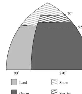
The DCESS model consists of one hemisphere, divided by 52◦latitude into a low–mid-latitude (LL) and a high-latitude (HL) zone (Fig. 2). Sea ice and snow cover are diagnosed from estimated meridional profiles of atmospheric tempera-ture (see below). Values for global reservoirs, transports and fluxes are obtained by doubling the hemispheric values. For the atmosphere module we use a simple, zonal mean, en-ergy balance model for the near-surface atmospheric temper-ature, forced by yearly-mean insolation, outgoing longwave radiation, meridional sensible and latent heat transports and air–sea heat exchange (Fig. 3). In combination with the sim-ple sea ice and snow parameterizations, the model includes the ice/snow albedo feedback and the insulating effect of sea ice. Prognostic equations for mean atmospheric temperature in each zone are obtained by integrating the energy balance over the zones. Meridional variations of atmospheric temper-ature are represented by a second order Legendre polynomial in sine of latitude, adjusted to fit zonal mean temperatures. Temperatures and gradients at the 52◦dividing latitude from this meridional profile are used in the calculation of merid-ional transports of sensible heat, latent heat and water vapor. The atmosphere exchanges heat and gases with the ice-free part of the ocean (Fig. 3). Gases are taken to be well-mixed in the atmosphere and those considered are carbon dioxide and methane (for all three carbon isotopes), nitrous oxide and oxygen. Methane is oxidized to carbon dioxide on timescales on the order of 10 years, increasing as methane concentra-tions increase (see below). In this original model, air–sea ex-change of methane is not considered. The model also deals
Figure 2.Model configuration. The model consists of one hemi-sphere divided by 52◦ latitude into 360◦ wide, low–mid-latitude (LL) and high-latitude (HL) sectors. Values for global reservoirs, transports and fluxes are twice the hemispheric values. The model ocean is 270◦wide and extends from the Equator to 70◦latitude. The ocean covers 70.5 % of the model surface. LL and HL ocean sectors have the area ratio 84:16. Sea ice and snow coverage are diagnosed from idealized, meridional profiles of atmospheric tem-perature.
with oxygen isotopes in atmospheric water vapor. Prognostic equations for atmospheric gases follow from internal sinks, exchanges with ocean surface layers and the land biosphere as well as input/outputs from weathering and lithosphere out-gassing.
The model ocean is 270◦wide, extends from the Equator to 70◦latitude and covers 70.5 % of the Earth surface (Fig. 2). Both the LL and HL ocean sectors have 55 vertical layers with 100 m resolution. An ocean sediment sector is assigned to each of the ocean layers with widths representing modern day hypsography (Fig. 3). Ocean circulation and mixing is characterized by four parameters:
1. A transport,q, associated with HL sinking and the deep-est LL upwelling.
2. Constant horizontal diffusion between the zones, Kh,
associated with the wind-driven circulation and deep re-circulation.
3. Strong, constant vertical diffusion in the HL zone,KvHL, associated with high-latitude convection.
4. A weak, depth-dependent vertical diffusion in the LL zone,KvLL.
Figure 3.Atmosphere, ocean and ocean sediment configurations. Temperatures of low–mid (LL) and high (HL) latitude atmosphere sectors derive from energy balance forced by yearly-mean insolation (SW), outgoing longwave radiation (LW), meridional transports of sensible (SH) and latent (LH) heat, and air–sea heat exchange (H). In combination with the simple sea ice and snow (hatched bars) parameterizations, the model includes the ice/snow albedo feedback and the insulating effect of sea ice. Meridional variations in atmospheric temperature are represented by a second order Legendre polynomial in sine of latitude, adjusted to fit sector mean temperatures. Temperatures and gradients at the 52◦ dividing latitude from this meridional profile are used to calculate sensible heat, latent heat and water vapor transports. The atmosphere exchanges heat and gases (G) with the ice-free part of the ocean. Gases are well-mixed in the atmosphere and their concentrations follow from internal sinks, exchanges with ocean surface layers and the land biosphere and input/outputs from weathering and lithosphere outgassing. Both LL and HL ocean sectors are continuously stratified with 100 m vertical resolution to maximum depths of 5500 m and each sector has a bottom topography based on real ocean depth distribution. Model ocean circulation and mixing are indicated by the black arrows and associated circulation/mixing type labels (see main text). Model ocean biogeochemical cycling is indicated by the colored arrows (acting in both sectors but for simplicity only shown for LL sector) and associated matter (particulate organic, POC; biogenic carbonate, PIC; and inert mineral, NCM). Each of the 110 model sediment segments has an area set by the real ocean depth distribution and consists of a 10 cm thick, bioturbated layer divided into seven sublayers. Sediment biogeochemical cycling is indicated by colored arrows and associated matter. Exchange of dissolved species at the sediment–water interface is also indicated. The sedimentation rate down out of the bioturbated layer (ws) is calculated from mass conservation.
production of particulate organic matter depends on surface-layer phosphate availability but with lower efficiency in the HL zone. The calcite to organic carbon rain ratio depends on surface-layer temperature. Remineralization and dissolu-tion of particles falling down out of the ocean surface are described by exponential functions with depth. Prognostic equations for each of the tracers in each of the ocean lay-ers follow from ocean transport and mixing, internal sinks and sources, and exchanges with the ocean sediment. Ocean surface layers are also acted upon by exchanges with the at-mosphere and river inputs associated with weathering.
The semi-analytical ocean sediment module considers cal-cium carbonate dissolution and both oxic and anoxic organic matter remineralization. The sediment is composed of cal-cite, non-calcite mineral and reactive organic matter. Sedi-ment porosity profiles are related to sediSedi-ment composition and a bioturbated layer 0.1 m thick is applied. Carbonate and
organic carbon burial are calculated from sedimentation ve-locities at the base of the bioturbated layer. Bioturbation rates and oxic and anoxic remineralization rates depend on or-ganic carbon rain rates and dissolved oxygen concentrations. The land biosphere module considers leaves, wood, litter and soil. Net primary production depends on atmospheric carbon dioxide concentration, and remineralization rates in the litter and soil depend on mean atmospheric temperatures. Methane production is a small, fixed fraction of the soil remineraliza-tion. The lithosphere module considers outgassing, weather-ing of carbonate and silicate rocks, and weatherweather-ing of rocks with old organic carbon and phosphorus. Weathering rates are related to mean atmospheric temperatures.
those of the best other Earth system models of intermediate complexity as seen in recent intercomparison studies of past, present and future carbon cycling and climate (Eby et al., 2013; Joos et al., 2013; Zickfeld et al., 2013). The results from these studies were also included in the recent Fifth Assessment Report of the Intergovernmental Panel for Cli-mate Change (IPCC, 2013). From the 2013 studies onward, the carbon fertilization parameter of the terrestrial biosphere module was decreased somewhat in the model (Eby et al., 2013).
The Paleocene–Eocene Thermal Maximum (PETM) warming event 56 million years ago was addressed in the most recent model application (Shaffer et al., 2016) whereby the very simplified methane cycling sketched above was im-plemented and the carbon input was taken to occur over a 10 000-year timescale. That is significantly longer than timescales associated with methane oxidation in the atmo-sphere or ocean overturning, and the system response is rather insensitive to input type and location (ocean or atmo-sphere). Therefore, for simplicity the carbon input was taken to be in the form of carbon dioxide that was injected into the atmosphere. To deal with this deep-time warming event, several other modifications were made to the basic DCESS model (Shaffer et al., 2016):
1. The solar constant was decreased by 0.5 % from present day, sea level was raised by 100 m while retaining the modern day hypsography, and mean ocean salinity was taken to be 33.8 (the modern value is 34.7).
2. Background albedo was reduced due to less land at sub-tropical latitudes and more vegetation cover.
3. Initial land biomass was increased to reflect more land at low and mid-latitudes.
4. To account for high-latitude cloud forcing, extra forcing was imposed poleward of the latitude of sea ice extent in the standard model, pre-industrial steady state. 5. Parameters in the simple Budyko-type formulation for
outgoing longwave radiation (Budyko, 1969) were ad-justed in concert with the other forcing changes to achieve late Paleocene temperatures and climate sensi-tivity estimates.
6. Ocean calcium and magnesium concentrations were ad-justed to late Paleocene values.
7. Model weathering formulation was extended to include the size of the weathering substrate, estimated for the late Paleocene to be less than that for the present. 8. Lithosphere outgassing was increased to conform to late
Paleocene estimates.
9. The formulation of the calcite to organic carbon rain ra-tio was extended to also depend on the calcite saturara-tion state of the ocean surface layer.
10. The dependence of carbon isotope discrimination dur-ing ocean surface-layer photosynthesis was extended to depend on concentrations of dissolved carbon dioxide and phosphate there.
3 Methane cycling implementation 3.1 Atmosphere
For an oxygenated atmosphere, the dominant sink for atmo-spheric methane is oxidation to CO2 by reaction with the
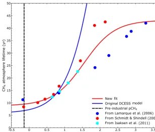
OH radical. Since this reaction depletes the concentration of these radicals, methane atmospheric lifetime, τ, grows as methane concentrations increase. In the original model (Shaffer et al., 2008), this effect and that of associated chem-ical reactions in the troposphere and stratosphere was ad-dressed by fitting results from a complex atmospheric chem-istry model (Schmidt and Shindell, 2003) to the equation
τ=τPI(M+b)/[(1−a)M+b], (1)
where τPI is the pre-industrial lifetime, a and b are
fit-ting constants andM≡(pCH4−pCH4,PI)/pCH4,PI, where pCH4 is the atmospheric partial pressure of methane and pCH4,PIis its pre-industrial value taken to be 720 ppb. The
Schmidt and Shindell (2003) target results and the model fit to them used in Shaffer et al. (2008) are shown in Fig. 4 (red dots and blue line). For this fitτPI=6.9 years,a=0.96 and b=6.6.
Figure 4 also shows results from several additional chem-istry modeling studies for the dependency of τ on pCH4
(blue dots from Lamarque et al., 2006; black dots from Isak-sen et al., 2011). For the range of low to medium methane concentrations considered in Schmidt and Shindell (2003) and Isaksen et al. (2011), these authors found rather low sen-sitivity of their results to atmospheric water vapor levels cit-ing methane lifetime changes of less than 10 % for tropo-spheric water vapor increases of 30–40 %. On the other hand, Lamarque et al. (2006) found that atmospheric lifetimes de-crease for extreme values ofpCH4 due to much more
en-hanced water vapor and OH production (and thereby greater methane oxidation) of a very warm climate. The red line in Fig. 4 shows a fit to all the chemistry modeling results of the figure using Eq. (1), a fit for whichτPI=9.5 years, a=0.78 andb=11. This new fit now also captures, in part, enhanced OH production and the associated limitation ofτ for very high values ofpCH4and has been adopted in our
en-hanced model whereby the model atmospheric methane sink in moles per year isυapCH4/τ withυa as the atmospheric
mole content.
(2006) (2003) (2011)
Figure 4.Atmospheric lifetime of methane as a function of atmospheric methane concentration. See text for a discussion of the model results and the functional fit to them.
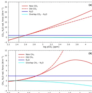
here. However, recent work has provided methane radiative forcing formulations, including nitrous oxide overlap, for methane concentrations up to 100 ppm (Byrne and Goldblatt, 2014a) and even up to 10 000 ppm (Byrne and Goldblatt, 2014b). We adopt these results and, for consistency, we also adopt the Byrne and Goldblatt (2014a) expressions for car-bon dioxide radiative forcing and for carcar-bon dioxide–nitrous oxide overlap. Figure 5 serves to illustrate these radiative forcings. Note that for very high methane concentrations, ra-diative forcing levels off and even decreases, an effect caused by enhanced shortwave absorption at such concentrations (Byrne and Goldblatt, 2014b). Taken together with the lev-eling off of methane atmospheric lifetimes at such concen-trations (Fig. 4), this limits the role that can be played by methane in enhancing global warming under such extreme conditions.
To illustrate the effects of these new radiative forcing for-mulations we consider several specific atmosphere composi-tions and the warming associated with them. If we consider an atmosphere withpCO2,pCH4andpN2O values of 500,
10 and 0.5 ppm, respectively, this corresponds to radiative forcings relative to pre-industrial conditions of 3.26, 2.32 and 0.73 W m−2but with a total forcing overlap of−0.16 W m−2, leading to a total forcing of 6.15 W m−2. With the origi-nal radiative forcing formulations used in the DCESS model (Myhre et al., 1998; Shaffer et al., 2008) the total radia-tive forcing is similar, 6.25 W m−2. For a nominal climate
sensitivity of 3◦C for apCO2doubling (0.81◦C W−1m−2),
such total forcings would lead to global mean temperature in-creases of 4.98 and 5.06◦C, respectively, above the DCESS pre-industrial mean global temperature of 15◦C. If we con-sider an atmosphere withpCO2,pCH4andpN2O values of
1000, 100 and 1 ppm, respectively, this corresponds to ra-diative forcings relative to pre-industrial conditions of 7.45, 6.50 and 1.88 W m−2 but with a total forcing overlap of
−0.93 W m−2, leading to a total forcing of 14.97 W m−2. With the original radiative forcing formulations, the total radiative forcing is considerably higher, 18.36 W m−2. For a 3◦C climate sensitivity, such total forcing would lead to global mean temperature increases of 12.13 and 14.87◦C, re-spectively; for a 5◦C climate sensitivity (Shaffer et al., 2016) the increases would be 20.22 and 24.79◦C, respectively. 3.2 Ocean
3.2.1 Simplified nitrogen and sulfur cycling
To be able to deal with suboxic and anoxic ocean conditions that would arise for significant oxidation of methane in the ocean interior, the model has been generalized to consider nitrogen and sulfur cycling with the introduction of nitrate (NO3), ammonium (NH4) and hydrogen sulfide (H2S) as
Red-Figure 5.Radiative forcing of carbon dioxide, methane and nitrous oxide as functions of their atmospheric concentrations.(a)CO2radiative forcing used here (new CO2; Byrne and Goldblatt, 2014a) compared to CO2forcing in the original DCESS model (old CO2; Shaffer et al., 2008). CO2–N2O overlap (Byrne and Goldblatt, 2014a) and N2O radiative forcing calculated for constant, pre-industrial N2O partial pressure of 270 ppb.(b)CH4radiative forcing used here (new CH4; Byrne and Goldblatt, 2014a, b) compared to CH4forcing in the original DCESS model (old CH4). CH4–N2O overlap (Byrne and Goldblatt, 2014a) and N2O radiative forcing calculated for constant N2O partial pressure as in(a).
field (mole) ratio, taken to be 16. Likewise, organic matter produced, remineralized or buried maintains this ratio of ni-trogen to phosphorus. Following Shaffer et al. (2008), we ne-glect dissolved organic matter such that the rate of export of particulate organic matter down out of the surface layer is equal to new production and we assume an exponential law for the vertical distribution of remineralization of “nutrient” and “carbon” components of this organic matter, each with a distincte-folding length,λNandλC, respectively.
Model new production of organic matter in the sur-face layer has been generalized to depend on the limit-ing nutrient, either phosphate or nitrate, such that NPl,h=
min(NPPl,h,NPNl,h), where NPPl,h,NPNl,h=
Al0,hnizeu(1, rNP)−1
Lfl,h/sy PO4l,h,NOl3,h nh
PO4l,h/PO4l,h+P1/2 i
,hNOl3,h/NOl3,h+N1/2 io
(2)
and l, h refer to LL and HL ocean zones,Al0,hniare the ice-free ocean surface areas,zeu is the surface-layer depth (100 m), rNPis a Redfield ratio (taken to be 16),syis the number of
seconds per year, POl4,hand NOl3,hare the surface layer, phos-phate and nitrate concentrations, and P1/2,N1/2are half
satu-ration constants (1, 16 µmol m−3).Ll,h
f are efficiency factors,
taken to be 1 and 0.36 for the LL and HL zones, respectively (Shaffer et al., 2008). This is how the model accounts for light and iron limitation in the HL zone.
The surface-layer sinks due to new production are−NPl,h for phosphate and−rNPNPl,hfor nitrate. Other source/sinks
and Redfield ratios are adopted from Shaffer et al. (2008). Since we will deal with water column denitrification, we also consider nitrogen fixation as a surface-layer source of nitrate when NOl3,hlevels there drop belowrNPPOl4,hor equivalently
when NPP>NPN. In that case, we take the rate of nitrogen fixation, NFl,h, to be
NFl,h=NF0 h
where NF0 has been chosen to be 1×10⁶moles NO3 per
second.
In the water column, remineralization takes place through oxidation of organic matter with dissolved oxygen as long as oxygen levels are above a certain minimum value O2,min,
chosen here to be 3 mmol m−3. Below that value, remineral-ization is assumed to occur by way of denitrification as long as nitrate levels exceed a certain minimum level NO3,min,
chosen here to be 0.03 mmol m−3. The oxidation equation for denitrification is taken to be
(C106H124O38)(NH3)16(H3PO4)+94.4HNO3→
106CO2+16NH3+47.2N2+H3PO4+109.2H2O. (R1)
Here, as for oxidation with dissolved oxygen in the original DCESS model (Shaffer et al., 2008), we consider that organic matter formed in the ocean surface layer consists of proteins and lipids in addition to carbohydrates and adopt the mean composition proposed by Anderson (1995). Such a composi-tion requires more oxygen for complete oxidacomposi-tion than carbo-hydrate alone would require (Anderson, 1995). This explains the enhanced nitrate sink in denitrification compared to stan-dard Redfield stoichiometry (factors 94.4 and 47.2 compared with 84.8 and 42.4 in Reaction R1).
When oxygen concentrations are below Omin and nitrate
concentrations are belowNmin, remineralization is assumed
to occur by way of sulfate reduction for which the oxidation equation is taken to be
(C106H124O38)(NH3)16(H3PO4)+44H2O+59SO24−→
106HCO−3 +59HS−+16NH3+H3PO4+47H+. (R2)
For the same reason as above, the sulfate sink is somewhat enhanced compared to standard Redfield stoichiometry (fac-tor 59 compared with 53 in Reaction R2). Note that the car-bon oxidation product in sulfate reduction is bicarcar-bonate that, as opposed to the carbon dioxide produced in denitrification, contributes to alkalinity as well as dissolved inorganic carbon (DIC). Both reactions show a minor contribution to alkalin-ity by way of ammonia production. In addition, for sulfate reduction with our organic matter model, the alkalinity de-crease from the production of hydrogen ions exceeds the al-kalinity increase from the production of bisulfide (HS−; by definition, alkalinity∝HCO−3+NH3+HS−−H+; Dickson,
1981). In summary, for our organic matter stoichiometry, we find alkalinity :DIC=0.151 and 1.038 for denitrification and sulfate reduction, respectively.
As shown in Reactions (R1) and (R2), NH3and HS−are
produced by denitrification and/or sulfate reduction. As we show below, additional bisulfide is produced by microbes for anoxic conditions by way of anoxic methane oxidation (AMO). In the model, these species are oxidized to nitrate and sulfate, respectively, when transported by advection and diffusion to oxygenated ocean layers where O2≥O2,min.
These oxidation reactions are NH3+2O2→NO−3 +H
++
H2O (R3)
and
HS−+2O2→SO24−+H +
. (R4)
Note that each of the reactions leads to an alkalinity decrease from production of hydrogen ions.
Oxygenation rates, 0oxl,h,n (in moles per second), are ex-pressed by
0ox,NHl,h 4,n, 0
l,h
ox,H2S,n= −V l,h n
[NH3]l,hn ,
HS−l,h
n
/τox,NS, (4)
where n is the layer number, Vnl,h are the layer volumes, [NH3]ln,h,HS−ln,h are the layer species concentrations and τox,NSis an ocean lifetime taken to be 200 days.
The simple ocean nitrogen and sulfur chemistry outlined above is intended to capture the most important processes that would occur in the ocean following a massive injection of methane without going into further details of the N and S cycles. Processes that are left by the wayside here include anaerobic ammonium oxidation (anammox), oceanic pro-duction of nitrous oxide and iron sulfide formation (Kuypers et al., 2003; Freing et al., 2012; Morse et al., 1987). Anam-mox has shown to be an important sink of nitrogen nutri-ents in the ocean but denitrification may still be the most important player here (Ward et al., 2009; Zehr and Kudela, 2011). Treatment of anammox and nitrous oxide would in-volve in-depth consideration of nitrogen cycling including nitrite production and consumption as well as approaches that transcend our simple, horizontally averaged model ge-ometry. This is beyond the scope of the present paper but is being addressed by our group in other DCESS model de-velopments in progress. Likewise, sulfide formation would require an explicit treatment of iron cycling, also beyond the scope of the model at present.
3.2.2 Methane oxidation and air–sea gas exchange We now include methane as a tracer in the ocean model acted upon by advection, diffusion, air–sea gas exchange and mi-crobial oxidation in the water column. Here we ignore any weak methane production that may take place in the sur-face ocean in anoxic microenvironments (Reeburgh, 2007) again with the goal of concentrating on massive methane in-jections. Oxidation of methane in oxygenated ocean layers (Ol2,,nh ≥O2,min) produces carbon dioxide and consumes
oxy-gen according to
CH4+2O2→CO2+2H2O. (R5)
Layer oxidation rates of methane under these conditions, 0oxl,h,CH
4,n, are taken to be 0oxl,h,CH
4,n= −V
l,h
n
[CH4]ln,h
/τox,CH4, (5)
From a joint analysis of ocean methane and chlorofluorocar-bons data, Rehder et al. (1999) found support for modeling methane oxidation as a first order process (Eq. 5) and deter-mined an oceanic methane lifetime of ∼50 years. A much shorter lifetime of∼4 months was deduced for strong, fast and localized methane emissions during the 2010 Deepwa-ter Horizon oil spill in the Gulf of Mexico (Kessler et al., 2011). Below we takeτox,CH4to be 50 years since this value
is likely more applicable to our global approach but in the following we also check the sensitivity of our results to the much shorter lifetime.
For suboxic/weakly anoxic conditions characterized by O2<O2,minand NO3>NO3,min, we adopt the following
re-action for nitrate-dependent microbial AMO (Raghoebarsing et al., 2006; Cui et al., 2015):
5CH4+8HNO3→5CO2+4N2+14H2O. (R6)
An alternative and slightly more energetic reaction involves nitrite, a species that we do not consider in our simplified nitrogen-cycling approach (Haroon et al., 2013).
For anoxic conditions for which O2<O2,minand NO3<
NO3,min, sulfate-dependent microbial AMO (Treude et al.,
2005; Cui et al., 2015) may be expressed as
CH4+SO−42→HCO3−+HS−+H2O. (R7)
Note that whereas nitrate-dependent AMO (Reaction R6) does not produce alkalinity, the production of bicarbonate and bisulfide in sulfate-dependent AMO (Reaction R7) is a strong alkalinity source leading to an alkalinity :DIC ratio of 2, considerably higher than for sulfate reduction of organic matter (Reaction R2). From carbonate chemistry, an increase in ocean alkalinity tends to depress dissolved carbon diox-ide concentrations in the ocean and, by way of air–sea gas exchange, also in the atmosphere.
Layer oxidation rates of methane for sulfate-dependent AMO,0anoxl,h ,CH
4,n, are taken to be 0anoxl,h ,CH
4,n= −V
l,h
n
[CH4]ln,h
/τanox,CH4, (6)
whereτanox,CH4is an ocean methane lifetime for anoxic
con-ditions (O2<O2,minand NO3<NO3,min) that may be
con-siderably longer than τox,CH4 since Reaction (R7) is much
less energetic than Reaction (R5) (Lam and Kuypers, 2011). To take this into consideration and to be consistent with much lower anoxic remineralization rates compared to oxic rates in the DCESS model sediment module (Shaffer et al., 2008), we adopt τanox,CH4 =0.1τox,CH4 or 500 years as our
stan-dard case. On the other hand, nitrate-dependent AMO (Re-action R6) is energetically similar to oxic methane oxidation (Reaction R5) so we take τox,CH4 for the methane lifetime
associated with nitrate-dependent AMO. Air–sea gas exchange for methane,9CHl,h
4, is calculated as 9CHl,h
4=k
l.h
w
ηlCH,h
4pCH4−[CH4]
l,h, (7)
where the gas transfer velocities kwl.h are 0.39u2(SclCH,h
4/660)
0.5 whereby ul,h are mean wind speeds
at 10 m above the ocean surface, taken to be 8 m s−1in both
zones, and SclCH4,h are Schmidt numbers for methane that depend on ocean surface-layer temperature (see below). The methane solubility, ηlCH4,h , was converted from the Bunsen solubility coefficients that depend on surface-layer tem-perature and salinity (Wiesenburg and Guinasso, 1979) to model units using the ideal gas mole volume. Furthermore, [CH4]l,his the dissolved methane concentration in the ocean
surface layers.
In recent work it was shown that the traditional calcula-tions ofScCO2 based on a third order polynomial of
surface-layer temperature (Wanninkhof, 1992) seriously underes-timated ScCO2 for temperatures (T) above 30
◦C (Gröger and Mikolajewicz, 2011). These authors proposed the form Sc=aexp(−bT )+cand fit that equation using experimen-tal data of Jähne et al. (1987) to find best fit values for CO2of 1956, 0.0663 and 142.6 fora, bandc,respectively.
Since we are dealing here with simulations of extreme global warming, we adopt this newScCO2 expression and fit here,
thereby superseding the traditionalScCO2 calculation
previ-ously used in our model (Shaffer et al., 2008). Gröger and Mikolajewicz (2011) did not consider methane but we di-rectly fit their proposed exponential function to the experi-mental data of Jähne et al. (1987) forScCH4 over 5◦C
in-tervals in the temperature range 0–40◦C. We found best fit values (R2=0.997) fora, b andc, respectively, such that ScCH4=1771 exp(−0.0650T )+128.8. We adopt this
rela-tionship here.
4 Sample simulations with methane cycling 4.1 Methane input specification
The rate of methane input, FCH4, we apply to the
atmosphere–ocean system is taken to be FCH4(t )=404F
tot CH4/(τin)
5exp(−6.27t /τ
in) , (8)
whereFCHtot
4 is the total input in Gt C, τin is a timescale in
years over which the first 75 % of the input is added andt is the time in years. This mathematical form has been used before within our group to characterize CO2input (Shaffer,
2009; Shaffer et al., 2016). As discussed in the Introduction section, the great bulk of both possible majorFCH4 sources
to fuel deep-time warming events (methane hydrate and ther-mogenic methane) are likely to enter via the ocean. Estimates of the timescale for the carbon input driving the deep-time global warming events have varied from years to tens of thou-sands of years (eg. Zeebe et al., 2009; Cui et al., 2011; Wright and Schaller, 2013). On the lower end of this timescale range, Earth system response toFCHtot
4 will vary significantly
in bubble plumes for example (McGinnis et al., 2006). Such response variation may be explained in part by much shorter timescales for methane oxidation to carbon dioxide (in both the atmosphere and ocean) than ocean diffusive and over-turning timescales. Escape to the atmosphere will cause im-mediate global warming since methane is a powerful green-house gas, much more so than carbon dioxide (Myhre et al., 1998). Oxidation of dissolved methane in the ocean will con-sume dissolved oxygen there (Reaction R5). For oxidation of large amounts of methane, suboxic or anoxic conditions may develop with complex nutrient and carbon cycling con-sequences, upon which we elaborate below. We address these questions here by taking the direct, undissolved methane es-cape to the atmosphere to be αFCH4 and the methane
dis-solution in the ocean to be (1−α)FCH4, whereby αis the
fraction of total input that directly enters the atmosphere. Furthermore, we must specify how methane dissolution is distributed between the two ocean sectors and among the 55 layers of each sector. Here we simply assume that 84 % of the dissolution occurs in the LL sector and 16 % in the HL sec-tor, a division that reflects model sector areas. Furthermore, we assume that the amount assigned to each sector is divided equally among the upper 30 model ocean layers, spanning the depth ranges over which methane hydrate and/or ther-mogenic methane inputs may be expected (e.g., Buffett and Archer, 2004; Svensen et al., 2004).
4.2 Pre-event steady state and a long sample simulation
In order to investigate the impacts of these model improve-ments on simulation results, we chose as an initial case study the late Paleocene (pre-PETM) configuration and associated model steady states constructed in Shaffer et al. (2016) but now including some changes like the adaption of the Byrne and Goldblatt (2014a) expressions for carbon dioxide radia-tive forcing and for carbon dioxide–nitrous oxide overlap. In this configuration we assume a solar constant decrease of 0.5 % from present day, sea level rise of 100 m, mean ocean salinity of 33.8, slightly reduced background albedo (to represent less land in the subtropics and more vegeta-tion cover), extra high latitude, longwave cloud forcing of 30 W m−2, pre-industrial atmospheric oxygen level, adjust-ments in ocean calcium and magnesium concentrations and adjustments in initial lithosphere outgassing and weather-ing inputs. Furthermore, parameters in the model’s simpli-fied treatment of outgoing longwave radiation were adjusted to yield a global mean temperature of 25◦C and a climate sensitivity in the range 4–5◦C for atmosphericpCO
2
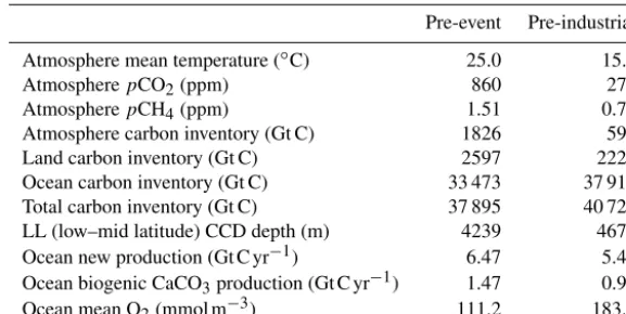
lev-els in the range 800–900 ppm (Shaffer et al., 2016). Open system steady states were then sought (by iteration and/or long time integration) such that external inputs (lithosphere outgassing and weathering) balanced external output (burial down out of the ocean sediment). Table 1 lists some proper-ties of the model steady state we chose among various pos-sibilities given the above constraints. This particular model
configuration with a global mean temperature of 25.0◦C and an atmosphericpCO2of 860 ppm has a climate sensitivity of
4.8◦C. While this steady state largely reflects late Paleocene conditions to ease comparison with our prior work, we em-phasize that a similar approach can be taken to design appro-priate initial conditions for any particular deep-time warming event, like the end-Permian event (Shen et. al., 2011), based on paleo-reconstructions for conditions prior to that particu-lar event.
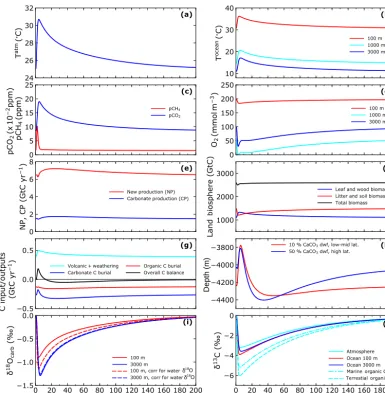
Figure 6 shows time evolutions of some relevant model variables from a 200 000-year simulation that started in equi-librium with the above initial conditions and was forced by methane input of 4000 Gt C over a timescale (τin) of 3 kyr,
whereby half of the input reaches the atmosphere and half is dissolved in the ocean (α=0.5). Furthermore, to be specific it is assumed that theδ13C of the methane input is−40 ‰. Such forcing leads to maximum event temperature andpCO2
rises of 5.7◦C and 1040 ppm, a peak atmosphericpCH 4 of
10.3 ppm and a LL calcite compensation depth (CCD) shoal-ing of 463 m (Fig. 6a, c and h).
The LL ocean warms by up to 5.5◦C at the surface, in-creasing to 6.0◦C at depth, reflecting modest polar ampli-fication of the warming by about 20 % (Fig. 6b). Mean LL dissolved O2concentrations at 1000 m depth approach 0
af-ter less than 2 kyr and remain so for an additional 3 kyr, driven, to a large extent, by oxidation of methane dissolved in the ocean (Fig. 6d). Considerable denitrification occurs during this 3 kyr long anoxic period, reflected in an associ-ated decrease in new production due to nitrogen limitation (Fig. 6e). After this decrease, ocean new production then steadily increases to about 12 % higher than pre-event lev-els by 24 kyr (due to more ocean phosphate from enhanced weathering) and then slowly decreases again as weather-ing decreases with temperature. There is only a slight ini-tial decrease of about 100 Gt C in land biosphere carbon inventory as more/less new production from CO2
fertiliza-tion was roughly balanced by more/less soil remineraliza-tion from warming/cooling (Fig. 6f). The initial decrease in both ocean new production and land biomass enhance atmo-sphericpCO2and warming while the subsequent ocean new
production increase followed by a slow decrease modulate the slow decrease inpCO2and slow cooling following peak
warming.
Weathering increases over the event are accompanied by an initial drop in carbonate burial as dissolution decreases the amount of sediment CaCO3 as well as the burial
ve-locity (Fig. 6g and h). There is little initial change in or-ganic carbon burial as the opposing effects tend to bal-ance: decreasing burial velocity and increased organic mat-ter preservation from decreasing O2concentrations. During
this period there is a net source of carbon to the ocean– atmosphere system (in addition to the prescribed methane input) as volcanic/weathering inputs exceed burial outputs. After the methane input event, both CaCO3and organic
Table 1.Pre-event steady-state solution properties compared to pre-industrial properties. CCD is the calcite compensation depth.
Pre-event Pre-industrial
Atmosphere mean temperature (◦C) 25.0 15.0
AtmospherepCO2(ppm) 860 278
AtmospherepCH4(ppm) 1.51 0.72
Atmosphere carbon inventory (Gt C) 1826 590 Land carbon inventory (Gt C) 2597 2220 Ocean carbon inventory (Gt C) 33 473 37 910 Total carbon inventory (Gt C) 37 895 40 720 LL (low–mid latitude) CCD depth (m) 4239 4673 Ocean new production (Gt C yr−1) 6.47 5.40 Ocean biogenic CaCO3production (Gt C yr−1) 1.47 0.97 Ocean mean O2(mmol m−3) 111.2 183.5
production. Together with decreasing weathering in response to cooling, this results in a weak but long-lived net sink of carbon from the ocean–atmosphere system (Fig. 6g). In combination with decreasingpCO2and associated
increas-ing ocean [CO23−], the biogenic CaCO3production increase
drives an overshoot of the LL CCD to depths greater than the pre-event depth, in agreement with theory and sediment core data (Dickens et al., 1997; Leon-Rodriguez and Dick-ens, 2010; Penman et al., 2016). This overshoot, which is even more pronounced at high latitudes, peaks by 35–45 kyr into the simulation (Fig. 6h).
The LL pelagicδ18O excursion in biogenic CaCO3is
sig-nificantly muted compared to the benthic one due to en-hancedδ18O in the surface layer (δ18Ow) from a more
vigor-ous hydrological cycle during the warming event (Fig. 6i) The carbon isotope excursion is slightly muted in the at-mosphere and enhanced in the LL ocean surface layer due to warming and temperature-dependent fractionation in air– sea gas exchange (Fig. 6j). The LL marine organic matter isotope excursion is greater still, in agreement with paleo-reconstructions (McInerney and Wing, 2011), as a conse-quence of model dependence of carbon isotope discrimina-tion during ocean photosynthesis on concentradiscrimina-tions of dis-solved carbon dioxide and phosphate in the ocean surface layer (Shaffer et al., 2016). Use of apCO2-dependent carbon
isotope fractionation leads to a still greater isotope excursion in terrestrial organic matter, also in agreement with paleo-reconstructions (Jahren and Schubert, 2013). Note that the model carbon isotope excursion is more protracted than the initial warming or theδ18O excursion related to the warm-ing (Fig. 6a, i and j). Relaxation back to about half of maxi-mum carbon isotope excursion values takes place over about 80 kyr compared to about 40 kyr for comparable temperature orδ18O relaxation. This can be explained by enhanced burial ofδ13C-enriched CaCO3after the methane input event. After
200 kyr, most of model Earth system properties have relaxed back toward pre-event values. This long timescale is dictated by external input/output balances of the global carbon cycle
(Fig. 6g), in particular by the slow, negative silicate weather-ing feedback on climate (Shaffer et al., 2008).
4.3 Sensitivity to input size, timescale and distribution
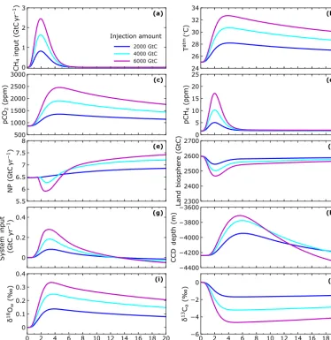
Figure 7 shows selected model results for the first 20 000 years of simulations like that of Fig. 6 but with methane input amounts of 2000, 4000 and 6000 Gt C. Both pCO2 and especiallypCH4 increase more than linearly in
response to the linear increase in methane input (Fig. 7a, c and d). For pCO2 this is due to positive feedbacks from
the land biosphere and ocean. Initial warming from the methane injection leads to greater soil remineralization, land carbon inventory decrease and input of CO2 to the
atmo-sphere (Fig. 7f). Increasing methane oxidation in the ocean leads to denitrification that draws down ocean new produc-tion leading to increased ocean CO2outgassing that was
al-ready enhanced in response to decreased ocean CO2
solu-bility from warming (Fig. 7e). The non-linear increase in pCH4is due mainly to the increase in CH4atmospheric
life-time withpCH4 (Fig. 4). On the other hand, warming
in-creases less than linearly (Fig. 7b) as expected from the radia-tive forcing dependencies shown in Fig. 5 and from our ne-glect here for simplicity of climate sensitivity increase with warming (Shaffer et al., 2016). Net carbon input from vol-canism/weathering minus burial follows process sequences as described for Fig. 6 above (Fig. 7g). The CCD shoals as more methane is oxidized to CO2 in the atmosphere and
ocean leading to more acidic conditions that drive calcite dis-solution in the sediment (Fig. 7h). However, CCD shoaling increase is damped for large methane dissolution in the ocean since this leads to anoxic conditions, methane oxidation with sulfate (Reaction R7) and associated alkalinity inputs that oppose dissolution. This also has had the effect of damp-ing the atmosphericpCO2increase. In response to warming,
p p
o o
b
δ18O
δ18O
Depth (m)
Figure 6. Results from a 200 000-year simulation with a methane input of 4000 Gt C over a timescale of 3000 years and with half the input dissolved in the ocean and half escaping as gas to the atmosphere.(a)Global mean atmospheric temperature,(b)LL ocean tempera-ture,(c)atmosphericpCO2andpCH4,(d)LL ocean-dissolved O2concentration,(e)ocean new and biogenic CaCO3production,(f)land biosphere carbon inventories for leaves+wood, litter+soil and their total, and(g)external input/outputs of carbon. The black line is vol-canic/weathering inputs minus burial outputs.(h)Depths to the LL 10 % (LL CCD) and HL 50 % CaCO3wt%,(i)LL excursions ofδ18O in biogenic CaCO3formed and those excursions corrected for excursions in ambientδ18Ow.(j)Carbon isotope excursions for the atmosphere, the LL ocean, LL marine organic carbon and terrestrial organic carbon (see text; the methane input hasδ13C= −40 ‰).
same reason and the salinity excursion can be approximated very well by multiplying the results in Fig. 7i by 2.8. At-mospheric carbon isotope excursion values are directly pro-portional to the size of the methane input and exhibit a long decay timescale as noted in Fig. 6 above (Fig. 7j):
Figure 8 shows selected model results for the first 20 000 years of simulations like that of Fig. 6 but with methane injection times τin of 300, 1000, 3000 and
10 000 years. For the shortest injection times, input rates in terms of carbon equal or exceed those of present-day anthro-pogenic carbon emissions exceeding 10 Gt C yr−1 (Fig. 8a; IPCC, 2013). Global warming spikes to much higher
val-ues for short injection times in response to large instanta-neous methane radiative forcing and under the influence of slow ocean exchange times (Fig. 8b and d). Warming tops out at 8.0, 6.7, 5.7 and 4.8◦C for the shortest to the longest injection times. Atmospheric pCO2 is also enhanced for
i
d
b
Figure 7.Results for 20 000-year simulations for different methane input amounts over a timescale of 3000 years and with half the in-put dissolved in the ocean and half escaping as gas to the atmosphere.(a)methane input rate,(b)global mean atmospheric temperature, (c)atmospheric partial pressure of carbon dioxide,(d) atmospheric partial pressure of methane,(e)total ocean new production,(f)total land biosphere biomass,(g)volcanic/weathering inputs minus burial outputs (as black line in Fig. 6g),(h)LL CCD depth (10 % CaCO3 dry weight in sediment),(i)oxygen isotope excursion of LL ocean surface-layer water, and(j)atmospheric carbon isotope excursion (the methane input hasδ13C= −40 ‰).
(Fig. 8a). One consequence of this situation is the muted CCD shoaling for shorter injection times following from en-hanced methane oxidation with sulfate (Reaction R7) and associated alkalinity inputs that oppose CaCO3 dissolution
(Fig. 8h). Both net carbon input and especially oxygen isotopes from LL ocean surface-layer water follow global warming due in large part to climate-dependent weathering and temperature-dependent atmospheric water vapor trans-port (Fig. 8a, g and i; Shaffer et al., 2008). The atmospheric carbon isotope excursion is much enhanced for short injec-tion times. This can be understood as follows: the carbon isotope signal from the methane injected to the atmosphere, and transferred there to CO2via oxidation of the methane,
builds up in the atmosphere and in the ocean surface layer
(not shown) due to long exchange times of about 1 kyr with the deep ocean (Fig. 8j). The atmospheric isotope excursion tops out at−5.24,−3.80,−3.21 and−3.03 for the shortest to the longest injection times.
Figure 9 shows selected model results for the first 20 000 years of simulations like that of Fig. 6 but with 0, 50 and 100 % of the methane input reaching the atmosphere (α=0, 0.5 and 1). Global warming, atmosphericpCH4and,
to a lesser extent, atmosphericpCO2are enhanced for more
input directly to the atmosphere (Fig. 9b–d). Warming is en-hanced by 1.7◦C for all methane input to the atmosphere compared to all input dissolved in the ocean. Even with all methane input dissolved in the ocean, atmosphericpCH4
b
d
Figure 8.Results for 20 000-year simulations for different methane input timescales for an input of 4000 Gt C with half the input dissolved in the ocean and half escaping as gas to the atmosphere. Properties plotted in(a–j)as in Fig. 7.
from the ocean via air–sea gas exchange (Fig. 9d). The pos-itive land biosphere feedback on atmospheric pCO2 is
en-hanced for all methane to the atmosphere due to enen-hanced warming (Fig. 9f). On the other hand, ocean feedbacks on at-mospheric pCO2are more nuanced. The positive solubility
feedback is enhanced for all methane to the atmosphere due to enhanced warming whereas the positive feedback from re-duced ocean new production is enhanced for all methane to the ocean (Fig. 9e). The latter effect is due to methane oxida-tion in the ocean leading to denitrificaoxida-tion and nitrogen limi-tation of new production. Increased CaCO3dissolution in the
ocean sediment is a further consequence of methane oxida-tion in the ocean when all methane is dissolved there. This leads to decreased calcite burial and enhanced net carbon input to the ocean–atmosphere system despite less weath-ering input from less global warming here (Fig. 9g). This also explains the enhanced CCD shoaling for all methane dissolved in the ocean (although modulated somewhat from
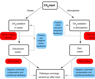
increased methane oxidation with sulfate and associated al-kalinity inputs as discussed above; Fig. 9h). Again, oxygen isotopes from LL ocean surface-layer water follow global warming due to temperature-dependent atmospheric water vapor transport (Fig. 9i). The atmospheric carbon isotope ex-cursion peaks slightly earlier for all methane to the atmo-sphere but, due to the long timescale of the methane input (3000 kyr) relative to ocean overturning times, the excursion amplitude is essentially the same for all cases (Fig. 9j). The flow diagram presented in Fig. 10 serves to compare and con-trast the pathways and feedbacks associated with (1) methane input to the ocean only and (2) methane input to the atmo-sphere only. These are the cases plotted as blue and maroon lines, respectively, in Fig. 9.
Figure 9.Results for 20 000-year simulations for different fractions of methane escape to the atmosphere for a methane input of 4000 Gt C over a timescale of 3000 years. Properties plotted in(a–j)as in Fig. 7. Also shown are results from a simulation with all methane input to the ocean (0 % fraction to atmosphere) and a much shorter ocean methane lifetime of 3 months (dashed blue lines; see main text).
Results for this new simulation are plotted as dashed blue lines in Fig. 9. The shorter lifetime leads to much re-duced methane concentrations in the ocean and less out-gassing to the atmosphere (Fig. 9d). Furthermore, faster methane oxidation in the ocean decreases dissolved oxygen there slightly, leading to slightly enhanced anoxia, sulfate-dependent anoxic methane oxidation and alkalinity inputs. As a consequence, CCD shoaling is damped somewhat as is the atmosphericpCO2increase (Fig. 9c and h). Together
with less methane outgassing, this leads to a reduction of maximum global warming of about 7 % compared to the standard case (Fig. 9b).
4.4 Modeled ocean distributions
Figure 11 shows selected LL model ocean results for the first 20 000 years of a simulation forced by a methane input
of 6000 Gt C withδ13C= −40 ‰ over a timescale (τin) of
3 kyr, whereby all the input is dissolved in the ocean (α=0). This forcing configuration was chosen to highlight the work-ings of the model for suboxic/anoxic conditions and leads to maximum event temperature andpCO2rises of 5.7◦C and
1095 ppm, a peak atmosphericpCH4of 6.2 ppm and a LL
CCD shoaling of 389 m (not shown).
LL ocean warming is greatest at depth, a reflection of polar amplification (Fig. 10a). Maximum warming there (6.2◦C) occurs about 1500 years after maximum surface-layer (or atmosphere) warming. Subsurface methane con-centrations build up to more than 30 mmol m−3(Fig. 11b).
Oxidation of this methane with dissolved oxygen (Reac-tion R5) forces suboxic condi(Reac-tions (O2<10 mmol m−3) for
Positive
feedbacks ocean negative
and warming
Fast, strong
warming Slower, weaker
ocean Oxic/anoxic
ocean Oxic
compensation and weathering feedbacks
Negative carbonate compensation and
weathering feedbacks Negative carbonate
Ocean Atmosphere
CH input4
Positive ocean
feedbacks and land biosphere CH oxidation
in ocean
CH oxidation
in atmosphere
Slow cooling Slow cooling
several kyr after input Pathways converge
4 4
Figure 10.Comparison of pathways and feedbacks for all methane injection into the ocean or into the atmosphere.
increased ocean new production (Figs. 5–7) maintains sub-oxic conditions at intermediate depths there well beyond the 20 000 simulation years shown here. As dissolved oxygen is forced below O2,min(3 mmol m−3), methane oxidation
pro-ceeds by way of nitrate-dependent anoxic methane oxida-tion (Reacoxida-tion R6), essentially eliminating nitrate for sev-eral thousand years at intermediate and mid-depths of the LL ocean (Fig. 11d). Over a period of several thousand years af-ter most methane is oxidized, nitrate concentrations recover to and even above pre-event values. This can be explained by a combination of nitrogen fixation (Eq. 3) and enhanced new production due to increased ocean phosphate concentrations from warming-enhanced weathering. As nitrate is forced be-low NO3,min(0.03 mmol m−3), methane oxidation proceeds
by way of sulfate-dependent anoxic methane oxidation (Re-action R7). This leads to the production of hydrogen sulfide that reaches concentrations over 10 mmol m−3at intermedi-ate depths almost 3 kyr into the simulation (Fig. 11e).
Figure 11f shows the model LL time–space distribution of omega () defined as the ratio of carbonate ion concen-tration to carbonate ion saturation concenconcen-tration for calcite. Calcite dissolution in the sediment increases asdecreases from 1 and model biogenic calcite production in the surface layer is proportional to(−1) /{1+(−1)}for≥1 and 0 for <1 (Shaffer et al., 2016). In response to methane oxidation to CO2, carbonate ions and therebyinitially
de-crease in intermediate and mid-depths where this oxidation occurs. However, as dissolved oxygen and nitrate are
con-sumed and sulfate-dependent anoxic methane oxidation takes over about 2 kyr into the simulation,increases in these lay-ers in response to alkalinity produced in this reaction. After the period of sulfate-dependent anoxic methane oxidation, decreases again followed by a slow increase driven by de-creasing CO2levels from carbonate compensation. LL
oxy-gen isotope excursions in biooxy-genic carbonate produced in situ (Fig. 11g) track temperature changes in the deep ocean but are reduced relative to these changes near the surface due to enhanced ambient water isotopes (Fig. 9i). After several thousand years, LL carbon isotope excursions in biogenic carbonate produced in situ (Fig. 11h) are slightly depressed in the deep ocean. This is due to dilution from additional less-depleted carbon inputs associated with sediment CaCO3
dissolution.
ex-Figure 11.LL ocean property results as functions of water depth and time for a 20 000-year simulation with a methane input of 6000 Gt C over a timescale of 3000 years, all of which dissolves in the ocean.(a)Temperature anomaly,(b)methane concentration,(c)dissolved oxygen concentration (model denitrification for O2<3 mmol m−3),(d)nitrate concentration (model sulfate reduction for NO3<0.03 mmol m−3), (e)hydrogen sulfide concentration,(f)omega, the ratio of carbonate ion concentration to the carbonate ion saturation concentration for calcite (see Fig. 11g),(g)oxygen isotope excursion in biogenic carbonate produced in situ.(h)Carbon isotope excursion. No corrections for the carbonate effect have been applied in(g)and(h)since these corrections were only derived for pelagic foraminifera (Spero et al., 1997).
change and the downwelling branch of the overturning circu-lation there (Fig. 12c). As a consequence, HL nitrate concen-trations remain elevated and there is no anoxic remineraliza-tion nor anoxic methane oxidaremineraliza-tion there (Fig. 12d). This also explains the essential lack of HL ammonium and hydrogen sulfate, <0.02 and <0.1 mmol m−3, respectively (Fig. 12e and f). Ammonium or hydrogen sulfate reaching the HL zone via horizontal exchange with the LL zone is quickly oxi-dized. By way of carbonate chemistry, addition of CO2 to
the water column via methane oxidation depresses carbonate ion concentrations (Fig. 12g). In terms of(see above) this reduction is relatively stronger in the HL surface layer, tend-ing to depress biogenic carbonate production there. However,
this reduction is largely offset by warming enhancement. Ad-dition of CO2 to the water column via methane oxidation
increases ocean acidity (Fig. 12h). For the simulation con-sidered here, surface-layer pH is reduced by 0.26 and 0.28 for the LL and HL zones, respectively, from pre-event levels already 0.47 and 0.48 lower than model pre-industrial levels (Shaffer et al., 2008).
4.5 Modeled ocean sediment properties and synthetic sediment cores
bio-Figure 12.Low–mid-latitude (LL) and high-latitude (HL) ocean property profiles at selected times for the simulation of Fig. 11. LL and HL results are plotted with red and blue lines, respectively. Line types for the selected times after the simulation start (0, 3 and 5 kyr) are defined in(a). COsat3 is the carbonate ion saturation concentration for calcite.
turbated sediment layers, each 10 cm thick, as well as sed-iment properties exported down out of these layers. In the original model, synthetic sediment cores (SSC) produced in this way only contained information on calcite and organic matter content of the buried sediment (Shaffer et al., 2008). We have extended this treatment to include carbon and oxy-gen isotopes and report the first results of this here for bulk carbonate, in the form of calcite in the model. For each sed-iment layer we consider conservation of calcite as well as conservation of carbon and oxygen isotopes in this calcite. This involves tracking the time-dependent inputs (from the rain of biogenic calcite produced in the ocean surface layer) and outputs (dissolution within the sediment layer and export down out of the layer by burial). Isotope effects for changes in surface-layer CO23−are applied in the production of
bio-genic calcite (Spero et al., 1997). The new model extension also accounts for effects of possible “mining” of buried sed-iment (i.e., upward directed “burial” velocities) in response to very strong dissolution events (Shaffer et al., 2008). For this, properties buried in each SSC are recorded to provide correct values for properties reentering the active sediment layer from below during any such “mining” event.
Figure 13.Comparison of bulk carbonate results from model synthetic ocean sediment cores at 3000 m depth with ocean surface-layer properties for the simulation of Fig. 11. Low–mid-latitude (LL) and high-latitude (HL) results are plotted with red and blue lines, respectively, and the methane input hasδ13C= −40 ‰.(a)Burial (downward) velocity relative to the base of the bioturbated sediment layer vs. synthetic sediment depth (SSD). SSD is referenced to zero at the start of the simulation and increases downcore by convention,(b)carbonate dry weight fraction vs. SSD,(c)LL bulk carbonateδ13C excursion vs. LL SSD (solid line). Also shown are theδ13C excursions in biogenic carbonate in the LL ocean surface layer (dashed line) and thisδ13C including the correction for change in surface-layer CO23− (dotted line; Spero et al., 1997), both plotted vs. simulation time (right sideyaxis). The time axis is “stretched/squeezed” relative to the SSD axis, a product of time-varying burial rates,(d)LL bulk carbonateδ18O vs. LL SSD (solid line). Also shown are (1) ocean surface-layer temperature anomaly (dashed line) on a temperature scale (topxaxis) related to the oxygen isotope scale (bottomxaxis) using temperature dependence of biogenic carbonateδ18O (Bemis et al., 1998), (2)δ18O in biogenic carbonate produced in the LL ocean surface layer (dashed-dot line) that includes the waterδ18O excursion (see Figs. 7–9i) and (3) thisδ18O including the correction for change in surface-layer CO23−(dotted line; Spero et al., 1997), all plotted vs. simulation time,(e)as(c)but for the HL ocean and sediment,(f)as(d)but for the HL ocean and sediment.
warmer than for the pre-industrial simulation (Shaffer et al., 2008). For this reason and due to slightly higher new pro-duction (Table 1), pre-event HL biogenic calcite rain is more than 3 times greater than for the pre-industrial case. On the other hand, pre-event, LL biogenic calcite rain is only about 15 % greater than for this case. Over the first 20 kyr of the simulation shown here, 38.7 cm of sediment is laid down at 3000 m depth in the HL zone compared to 14.0 cm in the LL zone. Burial velocities and sediment calcite content decrease initially in response to increased dissolution and, to a lesser extent, decreased rain rate, as a consequence of the methane
input and its oxidation in the ocean. Later on, both proper-ties increase to exceed their pre-event levels in response to increasing new production from increasing ocean phosphate levels.
in-put to it). The reservoir effect also leads to somewhat dis-tended bulk carbonate excursion maxima centered 3–4 kyr after surface-layer maxima (note that the time axis of the fig-ure is “stretched/squeezed” relative to the sediment length axis, a product of time-varying burial rates). Similar conclu-sions and interpretations also apply to the oxygen isotope ex-cursions in the SSC bulk carbonate and the ocean surface lay-ers in both model zones (Fig. 13d and f). Note that if, in lack of further knowledge, a linear timescale would be assigned to SSC length, the bulk carbonate excursions would appear sharper and shorter, particularly in the HL zone. When used as a paleothermometer, SSC bulk carbonate in the LL zone severely underestimates the model temperature excursion in the LL surface layer, primarily due to the positive ambient waterδ18O excursion demonstrated above, but with a minor contribution from the CO23−isotope effect (Fig. 13d). On the other hand, the slightly negative ambient waterδ18O excur-sion in the HL surface layer and the CO23−isotope effect there work to improve the estimate of the surface-layer warming from theδ18O excursion of SSC bulk carbonate, albeit with the 3–4 kyr time lag due to the reservoir effect (Fig. 13f).
5 Discussion and conclusions
Here we have extended the DCESS Earth system model to include methane cycling. This is a necessary step for dealing with deep-time global warming events, some of which cor-respond to major life extinction events, since most of these warming events were probably forced by massive methane inputs (Berner, 2002; Hesselbo et al., 2000; McElwain et al., 2005; Retallack and Jahren, 2008; Ruhl et al., 2011; Svensen et al., 2004; Shaffer et al., 2016). To be able to treat impacts of such inputs more correctly and consistently, we have also extended the model to deal with suboxic/anoxic conditions in the ocean and their consequences. For this we have now in-cluded denitrification, nitrogen fixation, sulfate reduction and nitrate/sulfate-dependent anoxic methane oxidation. Further-more, we have upgraded the treatment of methane for high concentrations in the model atmosphere with the latest radia-tive forcing relationships and with improved relationships for atmospheric lifetimes. To our knowledge, no other Earth sys-tem model of any degree of complexity has yet been formu-lated that can deal as comprehensively with extreme methane inputs and their Earth system consequences.
After formulating the model extensions we embark on ex-tensive tests of model behavior for methane inputs of vari-ous sizes, timescales and locations. We demonstrate model behavior over event timescales exceeding 100 kyr but con-centrate on the first 20 kyr of the simulations. The long, >100 kyr, simulation demonstrates how warming-driven weathering increases lead to a slow buildup of ocean phos-phate concentrations and ocean new production. This mod-ulates the evolution of atmospheric pCO2 and helps to
ex-plain model CCD deepening overshoot after the initial CCD
shoaling from the methane input. Extensive ocean anoxia develops for larger methane inputs over shorter timescales with more methane dissolving in the ocean. For such anoxia, there is much sulfate-dependent anoxic methane oxidation that produces hydrogen sulfide but also alkalinity that works to oppose calcite dissolution in the sediment and pCO2
rise in the atmosphere. Furthermore, extensive denitrification also occurs that initially depresses ocean new production, leading to pCO2 outgassing, until nitrogen fixation steps
in to fill the nitrate gap. The global warming excursion is greater when more methane escapes to the atmosphere, lead-ing to higherpCH4and more radiative forcing there. Initial
methane-driven warming forces increased soil remineraliza-tion and CO2input to the atmosphere until subsequentpCO2
rise and associated CO2fertilization turns the tables. Carbon
and oxygen isotope excursions of bulk biogenic carbonate in model SSCs are attenuated, distended and delayed relative to carbon and oxygen isotope excursions in the ocean surface layer where the carbonate is formed. Oxygen isotope excur-sions in surface-layer water compromise the use of oxygen isotope excursions in bulk carbonate to gauge surface-layer warming in the low-latitude ocean zone. However, such an oxygen-isotope-based paleo-thermometer works well in the HL ocean zone.