https://doi.org/10.5194/gmd-11-1887-2018 © Author(s) 2018. This work is distributed under the Creative Commons Attribution 4.0 License.
The Bern Simple Climate Model (BernSCM) v1.0: an extensible and
fully documented open-source re-implementation of the Bern
reduced-form model for global carbon cycle–climate simulations
Kuno M. Strassmann1,aand Fortunat Joos1,2
1Climate and Environmental Physics, Physics Institute, University of Bern, Bern, Switzerland 2Oeschger Center for Climate Change Research, University of Bern, Bern, Switzerland anow at: Institute for Atmospheric and Climate Science, ETH Zurich, Zurich, Switzerland Correspondence:Kuno Strassmann ([email protected])
Received: 22 September 2017 – Discussion started: 2 November 2017
Revised: 2 March 2018 – Accepted: 19 March 2018 – Published: 25 May 2018
Abstract. The Bern Simple Climate Model (BernSCM) is a free open-source re-implementation of a reduced-form car-bon cycle–climate model which has been used widely in pre-vious scientific work and IPCC assessments. BernSCM rep-resents the carbon cycle and climate system with a small set of equations for the heat and carbon budget, the parametriza-tion of major nonlinearities, and the substituparametriza-tion of complex component systems with impulse response functions (IRFs). The IRF approach allows cost-efficient yet accurate substitu-tion of detailed parent models of climate system components with near-linear behavior. Illustrative simulations of scenar-ios from previous multimodel studies show that BernSCM is broadly representative of the range of the climate–carbon cy-cle response simulated by more complex and detailed mod-els. Model code (in Fortran) was written from scratch with transparency and extensibility in mind, and is provided open source. BernSCM makes scientifically sound carbon cycle– climate modeling available for many applications. Support-ing up to decadal time steps with high accuracy, it is suit-able for studies with high computational load and for cou-pling with integrated assessment models (IAMs), for exam-ple. Further applications include climate risk assessment in a business, public, or educational context and the estimation of CO2and climate benefits of emission mitigation options.
1 Introduction
Simple climate models (SCMs) consist of a small number of equations, which describe the climate system in a spa-tially and temporally highly aggregated form. SCMs have been used since the pioneering days of computational cli-mate science to analyze the planetary heat balance (Budyko, 1969; Sellers, 1969) and to clarify the role of the ocean and land compartments in the climate response to anthropogenic forcing through carbon and heat uptake (e.g., Oeschger et al., 1975; Siegenthaler and Oeschger, 1984; Hansen et al., 1984). Due to their modest computational demands, SCMs en-abled pioneering research using the limited computational resources of the time and continue to play a useful role in the hierarchy of climate models today.
Recent applications of SCMs are often found in research in which computational resources are still limiting. Exam-ples include probabilistic or optimization studies involving a large number of simulations, or the use of a climate compo-nent as part of a detailed interdisciplinary model. SCMs are also much easier to understand and handle than large climate models, which makes them useful as practical tools that can be used by non-climate experts for applications for which detailed spatiotemporal physical modeling is not essential. This applies to interdisciplinary research, educational appli-cations, or the quantification of the impact of emission re-ductions on climate change.
mS1
Net air-to-sea carbon ux,fO
Radiative forcing Carbon dioxide
Non-CO₂ agents Carbon change
in surface ocean mS= ∑kmSk
ΔT1cS ΔT2cS Net air-to-sea heat ux, fOH
Global mean SAT change
ΔT = ∑kΔTk
mL1
aL1 . fNPP
Net primary productivity, fNPP mS1
1
τO1 1mS2 τ1mSk
Ok
mSn 1 τΟn
mL1 1 τL1
mLn 1 τLn
mL2 1 τL2
mLk 1 τLk mL2
aL2 . fNPP
mLk
aLk . fNPP
mLn
aLn . fNPP
Carbon in land biosphere mL = ∑k mLk
Emissions
Biomass decay, fdecay Regional climate
change Δv(x,t)
Pattern scaling
1 τO1ΔT1cS
1 τO2ΔT2cS
1 τOkΔTkcS
1 τOnΔTncS ΔTkcS ΔTncS
mS2 mSk mSn
aO2. fO
aO1. fO aOk. fO aOn. fO
aO2. fH O aO1. fH
O aOk. fHO aOn. fHO
τO2
Figure 1.BernSCM as a box-type model of the carbon cycle–climate system based on impulse response functions. Heat and carbon taken up by the mixed ocean surface layer and the land biosphere, respectively, is allocated to a series of boxes with characteristic timescales for
surface-to-deep ocean transport (τO) and of terrestrial carbon overturning (τL). The total perturbations in land and surface ocean carbon
inventory and in surface temperature are the sums over the corresponding individual perturbations in each box (mSk, 1Tk, mLk). Using
pattern scaling, the response in SAT can be translated to regional climate change for fieldsv(x, t )of variables such as SAT or precipitation.
to simulate emissions and their climate consequences. An-other application of simple models (e.g., Boucher and Reddy, 2008; Bruckner et al., 2003; Enting et al., 1994; Good et al., 2011; Hooss et al., 2001; Huntingford et al., 2010; Joos and Bruno, 1996; Oeschger et al., 1975; Raupach, 2013; Siegen-thaler and Oeschger, 1984; Smith et al., 2017; Tanaka et al., 2007; Urban and Keller, 2010; Wigley and Raper, 1992) is to compare, analyze, or emulate more complex models (Geof-froy et al., 2012a, b; Meinshausen et al., 2011; Raper et al., 2001; Thompson and Randerson, 1999). Simple models also play a significant role in previous assessments of the Inter-governmental Panel on Climate Change (e.g., Harvey et al., 1997). The comprehensive scope and interdisciplinarity of such models raise the challenge of maintaining a high and balanced scientific standard across all model components, es-pecially when human resources are limited. This may apply particularly to the climate component, as IAMs are mostly used within the economic and engineering disciplines. Cli-mate and carbon cycle representation are central parts of an IAM and have been critically assessed in the literature (Joos et al., 1999a; Schultz and Kasting, 1997; van Vuuren et al., 2011).
BernSCM is a zero-dimensional global carbon cycle– climate model built around impulse-response representations of the ocean and land compartments, as described previ-ously in Joos et al. (1996) and Meyer et al. (1999). The linear response of more complex ocean and land biosphere
models with detailed process descriptions is captured using impulse-response functions (IRFs). These IRF-based substi-tute models are combined with nonlinear parametrizations of carbon uptake by the surface ocean and the terrestrial biosphere as a function of atmospheric CO2 concentration and global mean surface temperature. Pulse response models have been shown to accurately emulate spatially resolved, complex models (Joos et al., 1996; Joos and Bruno, 1996; Meyer et al., 1999; Joos et al., 2001; Hooss et al., 2001).
solubility, are found to be smaller in magnitude than uncer-tainties arising from imperfect knowledge of surface-to-deep physical transport (see Fig. 2d and e in Friedlingstein et al., 2006). The exchange of CO2 between the atmosphere and the surface ocean is described by two-way fluxes, from the atmosphere to the surface ocean and vice versa, and the net flux of CO2into the ocean is proportional to the air–sea par-tial pressure difference. CO2reacts with water to form car-bon and bicarcar-bonate ions (Dickson et al., 2007; Orr et al., 2015), and acid–base equilibria are described here using the well-established Revelle factor formalism (Siegenthaler and Joos, 1992; Zeebe and Wolf-Gladrow, 2001). The first-order climate–carbon feedback of a decreasing solubility in warm-ing water is considered. Surface-to-deep exchange, the rate limiting step of ocean carbon and heat uptake, is described using an IRF. On timescales of up to a few millennia, pro-cesses associated with ocean sediments and weathering can be neglected. In such a closed ocean–atmosphere–land bio-sphere system, excess CO2is partitioned between the ocean and the atmosphere and a substantial fraction of the emit-ted CO2remains in the atmosphere and in the surface ocean in a new equilibrium (Joos et al., 2013). This corresponds to a constant term (infinitely long removal timescale) in the IRF representing surface-to-deep mixing. On multimillen-nial timescales, excess anthropogenic CO2is removed from the ocean–atmosphere–land system by ocean–sediment in-teractions and changes in the weathering cycle (Archer et al., 1999; Lord et al., 2016), and the IRF is readily adjusted to ac-count for these processes, important for simulations extend-ing over many millennia.
BernSCM simulates global mean surface temperature and the heat uptake by the planet. The latter is equivalent to the net top-of-the-atmosphere energy flux. Changes in the Earth’s heat storage in response to anthropogenic forcing are dominated by warming of the surface ocean and the interior ocean (T. F. Stocker et al., 2013) due to their large heat ca-pacity in comparison with that of the atmosphere and their large thermal conductivity in comparison to that of the land surface. Consequently, the atmospheric and land surface heat capacity is formally lumped with the heat capacity of the sur-face ocean in the BernSCM. The uptake of heat by the ocean (or planet) is, as for carbon, formulated as a two-way ex-change flux. The flux of heat from the atmosphere into the surface ocean is taken to be proportional to the radiative forc-ing resultforc-ing from changes in CO2and other agents (Etminan et al., 2016). The upward loss of heat from the surface is proportional to the product of the simulated surface temper-ature perturbation and the (prescribed) climate sensitivity λ
(Siegenthaler and Oeschger, 1984; Winton et al., 2010). As with carbon, surface-to-deep transport is the rate-limiting step for ocean heat uptake and thus for the adjust-ment of surface temperature to radiative forcing. This trans-port is key to determine the lag between realized warm-ing and equilibrium warmwarm-ing (Frölicher and Paynter, 2015). Again, this transport is described using an IRF. This IRF
en-capsulates the finite volume of the entire ocean. It also rep-resents the range of transport timescales associated with ad-vection, diffusion, and convection ranging from decades for the ventilation of thermocline to more than a millennium for deep Pacific ventilation as evidenced by transient tracers such as chlorofluorocarbons and radiocarbon (Olsen et al., 2016). The simulated surface ocean temperature perturbation, taken as a measure of global mean surface air temperature (SAT) change, may be combined with spatial patterns of change in temperature, precipitation, or any other variable of interest to compute regionally explicit changes (Hooss et al., 2001; Joos et al., 2001; B. D. Stocker et al., 2013) (Fig. 1).
Non-CO2 radiative forcing may be prescribed, e.g., fol-lowing estimates from complex climate–chemistry models (Myhre et al., 2013) or from simple emission-driven non-CO2 modules of radiative forcing related to CO2chemistry (Joos et al., 2001; Smith et al., 2017) and reconstructions of solar and volcanic forcing (Eby et al., 2012; Jungclaus et al., 2017) and considering the forcing efficacy of non-CO2 agents relative to CO2 forcing (Hansen et al., 2005). Climate sensitivity characterizing the response to radiative forcing is a free parameter in BernSCM. Climate sensitivity may change under increasing warming, particularly in high-emission scenarios (Geoffroy et al., 2012a; Gregory et al., 2015; Pfister and Stocker, 2017). Here, climate sensitivity is assumed to be time invariant and a potential state dependency of climate sensitivity is not considered. This may be changed when more solid information on state dependency becomes available or for the purpose of sensitivity analyses. Similarly, ocean heat uptake efficacy (Winton et al., 2010), influencing the atmospheric temperature response to ocean heat uptake forcing, is set to 1 here.
The present version 1.0 of BernSCM is fundamentally analogous to the Bern model as used already in the IPCC Second Assessment Report, Bern-SAR (whereas different versions of the Bern model family were used in the more recent IPCC reports). BernSCM represents the relevant pro-cesses more completely than Bern-SAR, thanks to additional alternative representations of the land and ocean compo-nents, which contain a more complete set of relevant sen-sitivities to temperature and atmospheric CO2.
Here, BernSCM model simulations are compared to pre-vious multimodel studies. The model is run for an idealized atmospheric pulse CO2 emission experiment of Joos et al. (2013), for an idealized CO2 forcing experiment similar to simulations from the Climate Model Intercomparison Project 5 (CMIP5), and for the SRES A2 emission scenario used in the C4MIP study (Friedlingstein et al., 2006).
steps are supported with high accuracy, suitable for the cou-pling with emission models of coarse time resolution, for ex-ample. However, the published code is a ready-to-run stand-alone model, which may also be useful in its own right.
BernSCM offers a physically sound carbon cycle–climate representation, but it is small enough for use in IAMs and other computationally tasking applications. In particular, the support of long time steps is ideally suited to the application of BernSCM as an IAM component, as these complex mod-els often use time steps on the order of 10 years.
BernSCM also offers a tool to realistically assess the cli-mate impact of carbon emissions or emission reductions and sinks, for example in aviation, forestry (Landry et al., 2016), blue carbon management, peat development (Mathi-jssen et al., 2017), life cycle assessments (Levasseur et al., 2016), or to assess the interaction of climate engineering in-terventions such as terrestrial carbon dioxide removal with the natural carbon cycle (Heck et al., 2016).
In this paper, we describe the model equations (Sect. 2 and Appendix), illustrative simulations in comparison with previ-ous multimodel studies, and uncertainty assessment (Sect. 3), followed by a discussion (Sect. 4) and conclusions (Sect. 5).
2 The BernSCM model framework and equations BernSCM simulates the relation among CO2 emissions, at-mospheric CO2, radiative forcing (RF), and global mean SAT by budgeting carbon and heat fluxes globally among the at-mosphere, the (abiotic) ocean, and the land biosphere com-partments. Given CO2emissions and non-CO2RF, the model solves for atmospheric CO2and SAT (e.g., in the examples of Sect. 3), but can also solve for carbon emissions (or residual uptake) when atmospheric CO2(or SAT and non-CO2RF) is prescribed, or for RF when SAT is prescribed.
The transport of carbon and heat to the deep ocean, as well as the decay of land carbon, results from complex but linear to first order behavior of the ocean and land com-partments. These are represented in BernSCM using IRFs (Green’s function). The IRF describes the evolution of a sys-tem variable after an initial perturbation, e.g., the pulse-like addition of carbon to a reservoir. It fully captures linear dy-namics without representing the underlying physical pro-cesses (Joos et al., 1996). More illustratively, the ocean and land models can be considered to consist of systems of un-coupled first-order ordinary differential equations or “box models”, which are an equivalent representation of the IRF model components (Fig. 1).
The net primary production (NPP) of the land biosphere and the surface ocean carbon uptake depend on atmospheric CO2and surface temperature in a nonlinear way. These es-sential nonlinearities are described by parametrizations link-ing the linear model components.
2.1 Carbon cycle component
The budget equation for atmospheric carbon is dmA
dt =e−fO−
dmL
dt , (1)
wheremA denotes the atmospheric carbon stored in CO2,e CO2 emissions,fO the flux to the ocean,mL the land bio-sphere carbon stock, andt time. Here,mLrefers to the (po-tential) natural biosphere. Human impacts on the land bio-sphere exchange including land use and land use changes are not simulated in the present version and are treated as ex-ogenous emissions (e). These emissions may be prescribed based on results from spatially explicit terrestrial models. An overview of the model variables and parameters is given in Tables A1 and A2.
The change in land carbon is given by the balance of NPP and decay of assimilated terrestrial carbon,
dmL
dt =fNPP−fdecay. (2)
Decay includes heterotrophic respiration (RH), fire, and other disturbances due to natural processes.
Carbon is taken up by the ocean through the air–sea inter-face (fO) and distributed to the mixed surface layer (mS) and the deep ocean interior (fdeep):
fO=
dmS
dt +fdeep. (3)
Global NPP (fNPP) is assumed to be a function of the par-tial pressure of atmospheric CO2(pCO2) and the SAT devia-tion from preindustrial equilibrium (funcdevia-tions for the imple-mented land components are given in Appendix A),
The net flux of carbon into the ocean is proportional to the gas transfer velocity (kg) and the CO2 partial pressure difference between surface air and seawater:
fO=kgAOε (pACO2−pCOS 2), (4)
whereAO is ocean surface area andεthe atmospheric mass of C per mixing ratio of CO2.
The global average perturbation in surface water1pCO2 S is a function of dissolved inorganic carbon change (1DIC) in the surface ocean at constant alkalinity (Joos et al., 1996) and SAT (Takahashi et al., 1993);1DIC andpCO2
A are related to model variables (see Appendix A),
1DIC= mS
HmixAO% Mµmol10−15Gt g−1
, (5)
pCO2
A =mAε
−1. (6)
The carbon cycle equation set is closed by the specification of
2.2 Climate component
BernSCM simulates the deviation in global mean SAT from the preindustrial state. SAT is approximated by the temper-ature perturbation of the surface ocean1T, which is calcu-lated from heat uptake by the budget equation
d1T
dt cS=f
H O −f
H
deep, (7)
wherecSis the heat capacity of the surface layer,fOHis ocean heat uptake, andfdeepH is heat uptake by the deep ocean (and accounts for the bulk of the effective heat capacity of the ocean). Continental heat uptake is neglected due to the much higher heat conductivity of the ocean in comparison to the continent.
fOHis taken to be proportional to RF (Forster et al., 2007) and the deviation of SAT from radiative equilibrium (1T = 1Teq(RF); see Table A2 for parameter definitions),
fOH=RF
1− 1T
1Teq
A
O
aO
. (8)
This relation follows from the assumption that feedbacks are linear in1T (e.g., Hansen et al., 1984).1Teqis given by
1Teq=RF1T2×
RF2×
, (9)
where1T2×is climate sensitivity (defined as the equilibrium
temperature change corresponding to twice the preindustrial CO2 concentration). Equation (8) describes ocean heat up-take as the difference between RF and the climate system’s response,λ·1T, withλ=RF/1Teqthe climate sensitivity expressed in W m−2K−1.
Climate sensitivity is an external parameter, as the model does not represent the processes determining equilibrium cli-mate response. RF of CO2 is calculated as (Myhre et al., 1998)
RFCO2=ln
pCO2
A
pCO2
A0 !
RF2×
ln(2), (10)
where pCO2
A0 is the preindustrial reference concentration of atmospheric CO2, and RF2× is the RF at twice the
prein-dustrial CO2 concentration. RF of other greenhouse gases (GHGs), aerosols, etc. can be parametrized in similar expres-sions involving GHG and pollutant emisexpres-sions and concentra-tions (Prather et al., 2001). In the provided BernSCM code, non-CO2RF is treated as an exogenous boundary condition. Total RF is then
RF=RFCO2+RFnonCO2. (11) The calculation of fdeepH (Sect. 2.3) completes the climate model.
2.3 Impulse response model components
The response of a invariant linear system to a time-dependent forcingf can be expressed by
m(t )=
t
Z
−∞
f (t0)r(t−t0)dt0. (12)
The functionris the system’s IRF, as can be shown by eval-uating the integral for a Dirac impulse (f (t0)=δ(t0)). The IRF indicates the fraction remaining in the system at timet
of a pulse input at a previous timet0. Because of linearity of the integral, any physically meaningful integrandf can be represented as a sequence of such impulses of varying size.
In BernSCM, an IRF is used to calculate the perturbation of heat and carbon in the mixed surface ocean layer (mixed layer IRF; Joos et al., 1996). For carbon,
mS(t )=
t
Z
−∞
fO(t0)rO(t−t0)dt0, (13)
and similarly, for heat
1T (t ) cS=
t
Z
−∞
fOH(t0)rO(t−t0)dt0. (14)
This approach has been shown to faithfully reproduce atmo-spheric CO2 and SAT as simulated with the models from which the IRF is derived (Joos et al., 1996). For temper-ature, the linear approach works since relatively small and homogeneous perturbations of ocean temperatures do not af-fect the circulation strongly and can be treated as a passive tracer (Hansen et al., 2010). Note that for compatibility with commonly used units, carbon fluxes are expressed in Gt yr−1, while heat fluxes are expressed in joules per second (watt) in Eqs. (13) and (14), respectively.
Equation (13) closes the ocean C budget equation (Eq. 3), as can be seen by taking the derivative with respect to time (usingr(0)=1),
dmS
dt =fO(t )−
−
t
Z
−∞
fO(t0)
drO dt (t−t
0
)dt0
| {z }
fdeep
, (15)
wherefdeepis the flux to the deep ocean. Similarly, Eq. (14) closes the heat budget equation (Eq. 7) for the surface ocean, d1T
dt cS=f
H O(t )−
−
t
Z
−∞
fOH(t0)drO
dt (t−t 0
)dt0
| {z }
fH deep
Another IRF is used for the carbon mL in living or dead biomass reservoirs of the terrestrial biosphere,
mL(t )=
t
Z
−∞
fNPP(t0)rL(t−t0)dt0. (17)
Again, Eq. (17) closes the budget equation for the land bio-sphere (Eq. 2), as shown by the derivative with respect to time,
dmL
dt =fNPP(t )−
−
t
Z
−∞
fNPP(t0)
drL dt (t−t
0
)dt0
| {z }
fdecay
. (18)
The time derivative of the land IRF is also known as the de-cay response function (e.g., Joos et al., 1996).
The IRFs above can be expressed as a sum of exponentials,
r(t )=a∞+
X
k
ake−t /τk, (19)
where the constant terma∞corresponds to an infinite decay
timescale.
The ocean IRF contains a positive constant coefficient
a∞, indicating a fraction of the perturbation that will remain
indefinitely (implied by carbon conservation in the ocean model). CaCO3 compensation by sediment dissolution and weathering (Archer et al., 1999) are not considered here, but could be described using analogous elimination processes with timescales on the order of 104to 105years (Joos et al., 2004). We emphasize that the implementation considering only the partitioning of excess carbon among atmosphere, land, and ocean (hencea∞6=0), neglecting ocean sediment
interactions and weathering flux perturbations, is only valid for timescales shorter than about 2000 years. In land bio-sphere models, in contrast, organic carbon is lost to the at-mosphere by oxidation to CO2at nonzero rates, and conse-quently all timescales are finite (i.e.,a∞=0), and the IRF
tends to zero (Fig. 2).
Inserting the formula (Eq. 19) in the pulse response equa-tion (Eq. 12) yields (f is a perturbation flux whena∞6=0)
m(t )=X
k t
Z
−∞
f (t0) ake−(t−t
0)/τ
kdt0+
t
Z
−∞
f (t0) a∞dt0. (20)
Thus the expression (Eq. 12) separates into a set of indepen-dent integralsmkcorresponding to the number of timescales
of the response. Taking the time derivative of the expres-sion (Eq. 20) reveals the equivalence to a system of uncou-pled first-order ordinary differential equations.
dmk
dt =f (t ) ak−mk/τk;
dm∞
dt =f (t ) a∞
m=X
k
mk+m∞ (21)
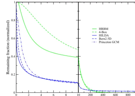
0 2 4 6 8 10
Time (yr) 0
0.2 0.4 0.6 0.8 1
Remaining fraction (normalized)
HRBM 4-Box HILDA Bern2.5D Princeton GCM
200 400 600 800 1000
Figure 2.IRFs of ocean (blue) and land (green) model compo-nents (without temperature dependence). Ocean compocompo-nents are normalized to a common mixed-layer depth of 50 m (multiplied by
Hmix/50 m), causing initial response to deviate from 1.
The direct numerical evaluation of Eq. (12) involves inte-grating over all previous times at each time step. The dif-ferential form Eq. (21) allows a recursive solution, which is much more efficient, especially for long simulations (the re-cursive solution implemented in BernSCM is described in Appendix B).
The differential equation system (Eq. 21) can be consid-ered to consist of several boxes, whereby each boxmk
re-ceives a fractionak of the input f and has a characteristic
turnover timeτk(Fig. 1). In the following this is referred to
as a box model. For the mixed ocean surface layer the carbon content of boxkis given by
dmSk
dt =fO(t ) aOk−mSk/τOk;
dmS∞
dt =fO(t ) aO∞ (22)
and the change in total carbon content in the mixed layer is
mS=
X
k
mSk+mS∞. (23)
Similar equations describe the heat content in the ocean sur-face layer, as well as the carbon stored in the land biosphere (Fig. 1).
functions to minimize the number of parameters needed for an accurate representation. In BernSCM, simple IRFs of the form (Eq. 19) are used exclusively. This allows adequate ac-curacy and a consistent interpretation as a multibox model.
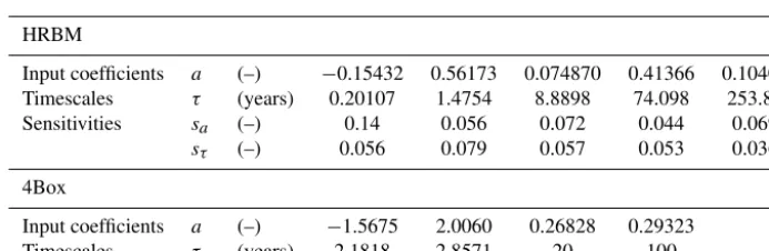
Thinking of IRF components as box models is concep-tually meaningful. The simple Bern 4-box biosphere model (Siegenthaler and Joos, 1992), for example, contains boxes corresponding to ground vegetation, wood, detritus, and soil (Appendix A). The High-Resolution Biosphere Model (HRBM) land component (Meyer et al., 1999), however, is abstractly defined by an IRF, but corresponds to boxes which correlate with biospheric reservoirs. However, since different box models may show a similar response, in practice the co-efficientsak and timescalesτk may not be uniquely defined
by the IRF and should be interpreted primarily as abstract fitting parameters (Enting, 2007; Li et al., 2009).
The IRF representation is, strictly speaking, only valid if the described subsystem is linear and the timescales of the system are time invariant. Then, the response functionr
does not depend on time and on state variables. In the Bern-SCM, major nonlinearities in the carbon cycle, namely air– sea gas exchange and the nonlinear carbonate chemistry, and changes in NPP in response to changes in environmental con-ditions are treated by separate nonlinear equations (Eqs. 4 and 5), while surface-to-deep ocean transport of carbon and heat and respiration of carbon in litter and soils are viewed as approximately linear processes using IRFs. However ocean circulation and the respiration of carbon from soil and litter is likely to change under global warming, violating the assump-tion of linearity. In practice, the IRF representaassump-tion remains a useful approximation as long as the impact of associated nonlinearities on simulated atmospheric CO2 and tempera-ture remain moderate.
The interpretation of the IRF representation as a box model provides a starting point for considering nonlinearities in the response. To account for nonlinearities, the response timescales τk and the coefficients ak may be gradually
ad-justed as a function of state variables such as temperature. As the integral form (Eq. 12) involves integration over the whole history at each time step, changing parameters along the way would result in inconsistencies. In contrast, the differential or box model form (Eq. 21) does not depend on previous time steps. Changing the model parameters from one step to the next thus equates to applying a slightly different model at each time step. Within each time step, the parameters remain constant, and the solution for the linear case applies. As time steps are small compared to the whole simulation, this dis-cretization yields accurate results, which is confirmed by the close agreement between the different time resolutions (Ta-ble B1).
Varying coefficients have been successfully implemented and tested for the HRBM land component and its decay IRF (Meyer et al., 1999). In this way, the enhancement of biomass decay by global warming is captured (see the Ap-pendix A and Sect. 3.1). In such a modification, the
advan-tage of the IRF and the equivalent box model representation – the faithful representation of the characteristic response timescale of a model system – is largely maintained, while at the same time the impact of time- and state-dependent sys-tem responses on simulated outcomes is approximated.
3 Illustrative simulations with the BernSCM 3.1 Model setup for sensitivity analyses and
uncertainty assessment
The carbon cycle–climate uncertainty of simulations with BernSCM can be assessed in two ways. First, to assess structural uncertainty, different substitute models for the ocean and land components can be used. Currently, this ap-proach is quite limited by the set of available substitute models (see Appendix A). Second, parameter uncertainty can be assessed by varying the temperature and CO2 sen-sitivities of the model, based on a standard set of compo-nents that represent the key dependencies as completely as possible (here, the IRF substitutes for the high-latitude ex-change/interior diffusion–advection (HILDA) ocean model (Joos et al., 1996) and for the HRBM land biosphere model (Meyer et al., 1999) are used in the standard setup).
The uncertainties of the global carbon cycle concern the sensitivity of the modeled fluxes of carbon and heat to chang-ing atmospheric CO2and climate. Key uncertainties strongly affecting the overall climate response are associated with land C storage: the dependency of NPP on CO2(CO2 fertil-ization), and the dependency of land C on temperature (fdecay increases with warming). This gives rise to large and op-posed carbon flux perturbations which are both very uncer-tain in magnitude (Le Quéré et al., 2016). While all substitute land models available for BernSCM include CO2 fertiliza-tion, only the HRBM substitute model represents tempera-ture sensitivity of biomass decay (Appendix A2).
As for the ocean, the uncertainty of heat uptake into the surface ocean is treated in terms of climate sensitivity (Eq. 8). The efficiency of the uptake of heat (fdeepH ) and carbon (fdeep) into the deep ocean is not sensitive to temperature, as the currently available substitute models all represent a fixed cir-culation pattern (IRF or box model parameters are not tem-perature dependent; Appendix A1). The nonlinear chemistry of CO2 dissolution in the surface ocean (Eq. 4), which de-termines the sensitivity of ocean C uptake to atmospheric CO2, is scientifically well established (Dickson et al., 2007; Orr and Epitalon, 2015) and is not treated as an uncertainty in BernSCM. The temperature sensitivities of NPP and CO2 dissolution in the surface ocean are treated as uncertain here, but have secondary influence on the climate response.
HILDA Bern2D Princeton
ECS 3.0 °C ECS 2.0 °C ECS 4.5 °C
ESMs EMICS
200 400 600 800 1000
0 50 100 150
Time (yr) 0
20 40 60 80 100
Fraction of realized warming (%)
200 400 600 800 1000
0 50 100 150
Time (yr) 0
20 40 60 80 100
Fraction of realized warming (%)
(a) (b)
Figure 3.Fraction of realized warming (temperature divided by the equilibrium temperature for the current RF) for idealized experiments
with prescribed atmospheric CO2concentration increase from preindustrial levels; panel(a)shows an exponential CO2increase by 1 % yr−1
over 140 years to approximately 4 times the preindustrial concentration (and linear increase in RF); panel(b)shows an abrupt increase to
4-fold CO2concentration. BernSCM simulations are shown for climate sensitivities of 2, 3, and 4.5 K and the three available ocean model
substitutes as indicated in the legend. Arrows in panel(a)indicate the corresponding warming fractions at year 99 compiled by Frölicher and
Paynter (2015, Tables 1, 2 in their Supplement) for Earth system models (ESMs, right-pointing) and Earth system Models of Intermediate Complexity (EMICs, left-pointing); arrow colors indicate climate sensitivities below 2.5 K (green), between 2.5 and 3.5 K (black), and above 3.5 K (red).
Coupled. All temperature and CO2 sensitivities are set to their standard values.
Uncoupled. All sensitivities are set to zero (except for the ocean CO2dissolution chemistry).
C-only. Only CO2dependencies are considered (CO2 fertil-ization).
T-only. Only temperature dependencies are considered in the land module (NPP, decay).
We performed simulations with these different setups. In Sect. 4.2, we probe the timescales of the temperature re-sponse in simulations in which atmospheric CO2is abruptly (instantaneously) quadrupled or by increasing CO2radiative forcing linearly within 140 years. In Sect. 4.3, we probe the response of the coupled system to a pulse-like release of 100 Gt C into the atmosphere. Finally in Sect. 4.4, we analyze carbon cycle–climate feedbacks relying on simulations over the industrial period and for the SRES A2 scenario. Bern-SCM results are compared with the results from three mul-timodel intercomparison projects: the Climate Model Inter-comparison Project 5 (CMIP5) with results as summarized by Frölicher and Paynter (2015), an analysis of carbon diox-ide and climate impulse response functions (Joos et al., 2013, here referred to as IRFMIP), and the C4MIP climate–carbon cycle feedback analysis (Friedlingstein et al., 2006).
3.2 Fraction of realized warming and idealized forcing experiments
The climate response of BernSCM is illustrated using ideal-ized simulations with prescribed forcing. One series of sim-ulations (a) was run for CO2 concentration increasing ex-ponentially from the preindustrial value by 1 % yr−1 over 140 years to approximately 4 times the preindustrial concen-tration, corresponding to a linear increase in RF (Fig. 3a); in a second series of simulations (b), CO2was abruptly in-creased to 4 times the preindustrial concentration (Fig. 3b).
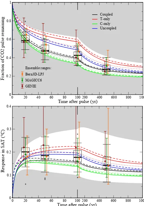
* **
* *
0 20 40 60 80 100
Time after pulse (yr) 0
0.1 0.2 0.3 0.4
Response in SAT (
°C
)
200 400 600 800 1000
0 20 40 60 80 100
Time after pulse (yr) 0
0.2 0.4 0.6 0.8 1
Fraction of CO2 pulse rem
aining
200 400 600 800 1000
Ensemble ranges: Bern3D-LPJ MAGICC6 GENIE
*
*
Coupled T-only C-only Uncoupled
Figure 4. IRFMIP pulse response range compared to BernSCM range for parameter uncertainty (colors according to legend) and structural uncertainty, with model versions HILDA–HRBM (solid lines), HILDA–4-box (dots), and Princeton–HRBM (dashed).
Stan-dard climate sensitivity is 3◦C, and a climate sensitivity range of 2–
4.5◦C is shown by the white area (envelope of all BernSCM runs).
Single-model ensemble ranges from IRFMIP are included as error bars indicating the 5–95 % range and dots indicating the median. The multimodel IRFMIP range is shown by box plots indicating median (bold black line), first quartiles (box), and extreme values (whiskers) excluding outliers deviating from the median by more than 1.2 times the interquartile distance (asterisks).
the ESMs (and lower on average than that of the EMICs). The validity of the IRF approach has also been shown by Good et al. (2011) using a SCM to reconstruct and inter-pret atmosphere–ocean general circulation model (AOGCM) projections. For the 150-year timescale of the CMIP5 exper-iments, Geoffroy et al. (2012a, b) show that the climate re-sponse of AOGCMs is well captured by a two-layer energy balance model with two effective response timescales.
In BernSCM, the fraction of realized warming depends primarily on the choice of climate sensitivity and is qualita-tively similar for the different model setups. Such a clear re-lationship is not seen in the EMS and EMICs. Thus the
struc-tural uncertainty and model differences of complex models are not fully represented in BernSCM. The BernSCM cli-mate response to abrupt warming (Fig. 3b) is qualitatively similar, especially on multicentennial timescales.
3.3 Impulse response experiment
Coupled carbon cycle–climate models can be characterized and compared based on their response to a CO2 emission pulse to the atmosphere (Joos et al., 2013). The airborne frac-tion (AF) denotes the fracfrac-tion of emissions found in the at-mosphere at a given time. In IRFMIP, the AF for a pulse of 100 Gt C, emitted on top of current (i.e., year 2010) at-mospheric CO2 concentrations, was simulated by a set of 15 carbon cycle–climate models of different complexity. For three of these models (Bern3D-LPJ, GENIE, MAGICC), en-sembles sampling the parameter uncertainty of these models are included in IRFMIP. Thus, IRFMIP captures structural as well as parameter uncertainty.
The IRFMIP pulse experiment was repeated with Bern-SCM, exploring parameter uncertainty of the carbon cycle (Sect. 3.1), as well as structural uncertainty, using the ocean model IRFs HILDA and Princeton (Sarmiento et al., 1992) in various combinations with the land biosphere components HRBM and the Bern 4-box model (Fig. 4). Simulations were run for equilibrium climate sensitivities of 3 (standard setup), 2, and 4.5◦C.
The AF simulated with BernSCM broadly agrees with the set of simulations from IRFMIP. At 100 years after the pulse, the AF is 0.40 (0.34–0.57) for a climate sensitivity of 3◦C (for coupled setup with uncertainty range in brackets). Cli-mate sensitivity uncertainty only slightly affects the upper end of this range (Fig. 4). For AF simulated with BernSCM, the standard coupled setup is close to the IRFMIP multi-model median. The BernSCM uncertainty range is asymmet-ric, like the IRFMIP multimodel range. For the MAGICC and GENIE ensembles, the medians also correspond with the BernSCM standard case, while the uncertainty ranges are more symmetric.
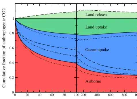
0 20 40 60 80 100 0
0.2 0.4 0.6 0.8 1
Cumulative fraction of anthropogenic CO2
200 400 600 800 1000
Time after pulse (yr)
Airborne Land uptake
Ocean uptake Land release
Figure 5.Land, ocean, and airborne fractions of the 100 Gt C CO2 pulse shown in Fig. 4 for the coupled (solid lines and colored ar-eas), T-only (dashed), C-only (dotted), and uncoupled (dash-dotted) model setups. In the T-only case, the land biosphere exhibits a net release (light green shading), and the ocean uptake consists of the sum of this area and the area delimited by the dashed line below the line at 1; for the uncoupled case, land uptake is zero and ocean uptake extends from the dashed–dotted line to unity.
ensembles (1.9–5.7◦C) and are compounded with RF differ-ences resulting from the uncertainty in atmospheric CO2.
Figure 5 shows how the added carbon is redistributed within the Earth system. In the coupled setup, the fraction of the initial pulse sequestered by the land and by the ocean increases over the first century, while the airborne fraction decreases. After 100 years, slightly more than 20 % of the added carbon is stored in the land and about 40 % in the ocean. The ocean continues to sequester excess carbon in the following centuries to become the dominant sink for excess carbon. In contrast, the land returns part of the sequestered carbon back to the atmosphere and ocean as decreasing at-mospheric CO2reduces the modeled CO2fertilization of the land biosphere. In the T-only setup, in which CO2 fertiliza-tion is not operating, the land is a source of carbon to the atmosphere due to accelerated soil turnover in response to warming. The largest land sink is simulated in the C-only setup, in which soil turnover timescales remain invariant and CO2fertilization is on. The different BernSCM setups span a range of plausible land biosphere and ocean responses to continued anthropogenic CO2 emissions as reflected in the simulated range in the airborne fraction (Figs. 4a and 5). 3.4 Carbon cycle–climate feedbacks
Climate models with explicit and detailed carbon cycle com-ponents exhibit a wide range of responses, as shown in the intercomparison studies of climate models with a de-tailed carbon cycle, C4MIP (Friedlingstein et al., 2006) and CMIP5 (Jones et al., 2013). The authors analyzed the
feed-back of carbon cycle–climate models using linearized sen-sitivity measures. These are derived from a simulation with temperature dependence (“coupled”) and one without (“un-coupled”; note that these names have a different meaning in BernSCM). Total CO2emissions for the coupled (left-hand side) and uncoupled (right-hand side) simulations can be ex-pressed as
1CAc (ε+βL+βO+α(γL+γO))=1CAu (ε+βL+βO), (24) where1CAis the cumulative change in atmospheric CO2(in parts per million) in the coupled (c) or uncoupled (u) cases, and the terms in parentheses represent the total sensitivity of C storage to1CA; in particular,βis the sensitivity of carbon storage to atmospheric CO2 (in Gt C ppm−1) on land (βL) or in the ocean (βO).γ is similarly the sensitivity in carbon storage to climate change, andα is the linear transient cli-mate sensitivity to CO2(◦C ppm−1) as in Friedlingstein et al. (2006);εconverts ppm to Gt C (see Table A2; the formula in the original paper implies identical units for atmospheric and stored carbon).
The climate–carbon cycle feedback is measured by the feedback metricg, defined by
1CAc
1CAu =
1
1−g (25)
and is thus estimated by
g= −α(γL+γO)
ε+βO+βL
. (26)
Thus the feedback strength scales with the assumed climate sensitivity and the temperature sensitivities and is reduced by CO2-induced sinks.
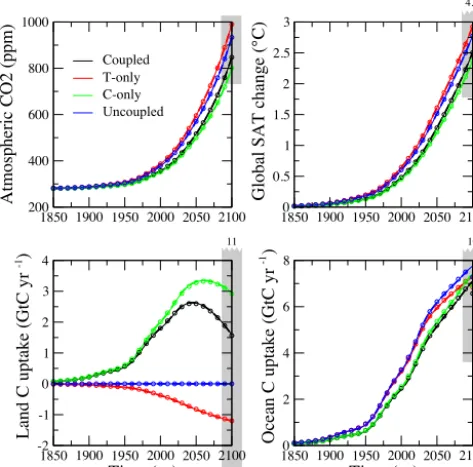
The C4MIP study used a SRES A2 emission scenario to compare the carbon cycle sensitivities of a range of mod-els. As in the C4MIP exercise, BernSCM was run for SRES A2 without any non-CO2 forcings (Fig. 6; prescribed his-torical and scenario emissions were smoothed with the R smooth.spline function (R Core Team, 2015) for 41 degrees of freedom for use with different time steps). Land use was treated as an exogenous CO2emission, while the land model simulates an undisturbed biosphere.
1850 1900 1950 2000 2050 2100 200
400 600 800 1000
Atmospheric CO2 (ppm)
Coupled T-only C-only Uncoupled
1850 1900 1950 2000 2050 21000 0.5
1 1.5 2 2.5 3
Global SAT change (°C)
1850 1900 1950 2000 2050 2100 Time (yr) -2
-1 0 1 2 3 4
Land C uptake (GtC yr )
1850 1900 1950 2000 2050 2100 Time (yr) 0
2 4 6 8
Ocean C uptake (GtC yr )
4.6
11
-6
10
-1 -1
Figure 6.BernSCM simulations of the SRES A2 scenario used for
C4MIP, with a climate sensitivity of 2.5◦C and the HILDA–HRBM
ocean–land components. Results for three numerical schemes are overlaid; (i) 0.1-year Euler forward time step (solid thin line), (ii) 1-year implicit time step (dashed bold line), (iii) 10-year implicit time step with piecewise linear approximation of fluxes (circles); the difference at this resolution is only visible in the C uptake. The C4MIP model range at 2100 is indicated by grey bars; numbers above or below the bars indicate values outside of the chart range.
warming. The resulting gaingis also smaller, though this re-sults in large part from the lower climate sensitivity in Bern-SCM (which corresponds to 2.5◦C as used for the Bern-CC model contribution to C4MIP). The lower end (in absolute terms) of the BernSCM carbon cycle sensitivity range is, however, zero per definition for all but the ocean-CO2 sen-sitivity βO (see Sect. 3.1). As a consequence, the climate– carbon cycle feedback range also includes zero. In contrast, the C4MIP range does not include zero for all sensitivity pa-rameters.
The land carbon uptake until 2100, under the different BernSCM configurations, varies over 500 Gt C (Fig. 6), more than 3 times the range of ocean uptake (180 Gt C). This partly reflects the limited coverage of the uncertainty in ocean mix-ing but also the fact that the land carbon sink is, together with the source related to land use, the most uncertain item in the budget (Le Quéré et al., 2009).
4 Discussion
We simulated illustrative scenarios from two recent multi-model studies, C4MIP and IRFMIP, to compare BernSCM to the literature of carbon cycle–climate models. The results
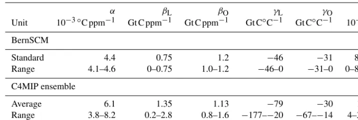
show that BernSCM is broadly representative of the current understanding of the global carbon cycle–climate response to anthropogenic forcing (in a time-averaged sense that does not address internal variability). The BernSCM uncertainty range in CO2 and SAT projections is broadly similar to the ranges spanned by probabilistic single-model ensembles and multimodel “ensembles of opportunity” such as the 15 IRFMIP models. The BernSCM uncertainty range shown consists mainly of parameter uncertainty and to a small ex-tent of structural uncertainty. For the standard coupled model setup, the sensitivities of ocean and land carbon uptake to changing CO2and climate (Table 1) of BernSCM are within the range of the detailed carbon cycle models in C4MIP. However, as some C4MIP models show much higher sensi-tivities, the BernSCM range does not capture the full C4MIP multimodel range. However, the C4MIP set is unlikely to sample uncertainty exhaustively, as each model contributed only a single, most likely simulation. Thus it does not include zero (or weak) sensitivities, whereas the BernSCM range does.
As Fig. 6 shows, solutions with different time steps and numerical schemes as implemented in BernSCM are largely equivalent for a sufficiently smooth forcing. This offers the flexibility to opt for simplicity of implementation or max-imum speed as required by the application (see also Ap-pendix B).
BernSCM does not explicitly distinguish between surface atmosphere and surface ocean temperature to compute global mean SAT perturbation. This is in contrast to some energy balance calculations used to analyze results from state-of-the-art ESMs (e.g., Geoffroy et al., 2012b). The BernSCM approach follows earlier work of Siegenthaler and Oeschger (1984). It is further guided by the similarity in reconstruc-tions of marine nighttime air and sea surface temperature perturbations (T. F. Stocker et al., 2013) that are consistent with the short, monthly relaxation timescale for air–sea heat exchange. The focus of the BernSCM is on the representation of the transport of heat from the surface into the thermocline and the deep ocean on decadal to multicentury timescales, while information on seasonal and spatial changes such as on land–sea air temperature differences or polar amplifica-tion may be obtained by applying suitable spatial perturba-tion patterns as derived from state-of-the-art models.
Currently, a limited set of substitute models is available and included with BernSCM. The simple structure and open-source policy of BernSCM allows users to address these cur-rent limitations according to the needs of their applications. More components can be added using the existing ones as a template. This requires the specification of the IRF and the parametrization of gas exchange for the surface ocean or NPP for the land biosphere (as described in Joos et al., 1996; Meyer et al., 1999).
trans-Table 1.C4MIP sensitivity metrics. The BernSCM range covers the carbon cycle settings as discussed in Sect. 3.1, and different combinations of model components (HILDA–HRBM, HILDA–4-box, Princeton–HRBM); the C4MIP range covers all participating models.
α βL βO γL γO g
Unit 10−3◦C ppm−1 Gt C ppm−1 Gt C ppm−1 Gt C◦C−1 Gt C◦C−1 10−2
BernSCM
Standard 4.4 0.75 1.2 −46 −31 8.3
Range 4.1–4.6 0–0.75 1.0–1.2 −46–0 −31–0 0–8.4
C4MIP ensemble
Average 6.1 1.35 1.13 −79 −30 15
Range 3.8–8.2 0.2–2.8 0.8–1.6 −177–−20 −67–−14 4–31
port parameters (aOk,τOk). It is in principle possible to repre-sent temperature dependency of ocean transport in a similar way as it is performed for the climate dependency of het-erotrophic respiration for the HRBM land biosphere substi-tute model (Meyer et al., 1999). In the current BernSCM ver-sion, the same IRF parameters are applied for the transport of carbon and heat from the surface ocean to the interior ocean. Thereby, it is implicitly assumed that the spatial pattern of change is the same for temperature and carbon. This appears to be a reasonable first-order approximation on decadal to century timescales as perturbations in temperature and car-bon show similar patterns with decreasing perturbations from the surface to depth. In future efforts, one may differentiate the ocean IRF for heat and carbon, in particular when more information from long-term multicentury to millennial-scale ESM simulations becomes available. The application of the same IRF for carbon and heat in individual model runs im-plies that modeled carbon and heat transport tend to be phys-ically consistent. In contrast, some other simple models em-ploy different transport parameters for heat and carbon and varied these parameters independently in probabilistic stud-ies.
A distribution of timescales applies to ocean transport pro-cesses as evidenced by observations of transient and time-dependent tracers such as chlorofluorocarbons and bomb-produced and natural radiocarbon and biogeochemical trac-ers (Key et al., 2004; Olsen et al., 2016). This continuum is sometimes approximated by one timescale, also termed heat uptake efficiency (e.g., Gregory et al., 2009), and by two timescales, as in Geoffroy et al. (2012b). The one-to-two timescale approximations were used to analyze relatively short ESM simulations that do not yet reveal the multicen-tury response timescales of the deep ocean. We note that the equivalent ocean depth of the simple energy balance model of Geoffroy et al. (2012b) for their AOGCM ensemble is only 1182 m compared to a mean ocean depth of about 3800 m. The ocean IRFs used in the BernSCM are derived from long simulations with ocean-only or simplified models. The range of distinct timescales used to construct the IRF faithfully ap-proximates the sub-annual to multicentury response
contin-uum of the parent models as shown in earlier work (Joos et al., 1996). Further, the BernSCM IRF model represents the heat capacity of the entire ocean.
The BernSCM model may be extended to model pertur-bation in the signatures and exchange fluxes of the carbon isotopes13C and14C as demonstrated in earlier work (Joos et al., 1996). This was not implemented here to keep the code as simple as possible and as most potential users are likely concerned with the evolution of climate and atmo-spheric CO2.
A potential future application of BernSCM is to use it as an emulator of the global long-term response of complex climate–carbon cycle models by adding the corresponding substitute model components. Additionally, pattern scaling can be applied to transfer the global mean temperature sig-nal into spatially resolved changes in surface temperature, precipitation, cloud cover, etc., exploiting the correlation of global SAT with regional and local changes (Hooss et al., 2001). This allows us to drive spatially explicit models, e.g., of terrestrial vegetation (as in Joos et al., 2001; Strassmann et al., 2008) or impacts related to climate change (e.g., as in Hijioka et al., 2009). Patterns of change are generally similar across models for temperature, whereas patterns in precipita-tion are more uncertain and show greater variability among models (Knutti and Sedlacek, 2013) and are forcing depen-dent (Shine et al., 2015). We also note that natural variabil-ity strongly influences the space-time evolution of climate change (Deser et al., 2012). Patterns may be scaled with changes in global mean SAT as indicated in Fig. 1 or depen-dencies on radiative forcing may be considered (Shine et al., 2015)
avail-able for observation-constrained probabilistic quantification of climate targets (Holden et al., 2010; Steinacher and Joos, 2016; Steinacher et al., 2013).
5 Conclusions
BernSCM is a reduced-form carbon cycle–climate model that captures the characteristics of the natural carbon cycle and the climate system essential for simulating the global long-term response to anthropogenic forcing. Simulated at-mospheric CO2concentrations and SATs are in good agree-ment with results from two comprehensive multimodel en-sembles. Process detail is minimal, due to the use of IRFs for system compartments that can be described linearly and nonlinear parametrizations governing the carbon fluxes into these compartments. This framework allows, in particular, the representation of the wide range of response timescales of the ocean and land biosphere and the nonlinear chemistry of CO2uptake in the surface ocean – both essential for reliably simulating the global climate response to arbitrary forcing scenarios.
Due to its structural simplicity and computational effi-ciency, BernSCM has many potential applications. In combi-nation with pattern scaling, BernSCM can be used to project spatial fields of impact-relevant variables for applications such as climate change impact assessment, coupling with spatially explicit land biosphere models, etc. With alterna-tive numerical solutions of varying complexity and stability to choose from, applications range from educational to com-putationally intensive integrated assessment modeling. Bern-SCM also offers a model-based alternative to global warming potentials for estimation of the climate impact of emissions and can be used to quantify climate benefits of mitigation options by applying emissions- or concentration-driven sim-ulations.
The generic implementation of linear IRF components offers a transparent, extensible climate model framework. Current limitations concern the number of available substi-tute models (limiting the uncertainty range represented), and ocean transport not influenced by climate change. An addi-tion of further alternative model components and more flex-ible representation of sensitivities in terms of continuously variable parameters would further increase the models’ use-fulness, for example for probabilistic applications.
Appendix A: Model parameters and parametrizations A1 Ocean
Currently available ocean components include substitute models for the high-latitude exchange/interior diffusion– advection model (HILDA Joos et al., 1996), Bern2D (Stocker et al., 1992), and the Princeton general circulation model (GCM) (Sarmiento et al., 1992). Ocean model parameters of the equations described in the main text are listed in Table A3 for the mixed-layer IRF/box models and in Table A2 for other equations. The IRF/box model parameters given here are recalculated by fitting a sum of six exponential functions and one constant to the original response functions as given in Joos and Bruno (1996). The original functions treated the first few years separately; the approximation to a purely ex-ponential form simplifies the equations and has a negligi-ble effect on accuracy. The parametrization of ocean surface CO2pressure is the same for all available ocean components and is given below.
Ocean surface CO2 pressure perturbations are fitted as a function of the globally averaged unperturbed surface tem-peratureT∗and perturbations in dissolved inorganic carbon (DIC) by Joos et al. (1996) using carbonate chemistry coef-ficients summarized by Millero (1995):
1 pCO2
S
T∗=(1.5568−1.3993×10
−2T∗
) 1DIC
+(7.4706−0.20207T∗)10−31DIC2
−(1.2748−0.12015T∗)10−51DIC3
+(2.4491−0.12639T∗)10−71DIC4
−(1.5468−0.15326T∗)10−101DIC5.
The expression holds for unperturbed global average sur-face water temperatureT∗between 17.7 and 18.3◦C and for
1pCO2
S between 0 and 1320 ppm.
Ocean surface CO2 pressure for global surface tempera-ture perturbation1T (Takahashi et al., 1993):
pCO2
S =p CO2 S
T∗·e
0.04231T.
A2 Land biosphere
Currently available land biosphere components include sub-stitute models for the High-Resolution Biosphere Model (HRBM) (Meyer et al., 1999) and the 4Box biosphere model (Siegenthaler and Joos, 1992).
For the HRBM model, temperature-dependent IRF/box model parameters as given by Meyer et al. (1999) are im-plemented:
eak=
akesakT
P
jajesajT ,
e
τk=τke−sτkT,
whereeak,eτkare the adjusted andak,τk the unperturbed pa-rameters. The IRF/box model parameter values for HRBM and the 4Box model are listed in Table A4. The temperature sensitivities of the HRBM IRF are parametrized for a warm-ing of up to 5◦C.
Net primary production for HRBM is given by (Meyer et al., 1999)
NPP(p)|1T=0= −e3.672801+e−0.430818·p −e−6.145559·p2+e−12.353878·p3 −e−19.010800·p4+e−26.183752·p5
−e−34.317488·p6−e−41.553715·p7 +e−48.265138·p8−e−56.056095·p9 +e−64.818185·p10,
wherepis atmospheric CO2pressure. This expression holds up to a CO2concentration of 1274 ppm and is capped at that value. The model includes growth enhancement by SAT in-crease (but without a dynamical vegetation):
NPP(p, 1T )=NPP0
·(1+0.11780208 tanh(1T /50.9312421) +0.002430513·tanh(1T /8.85326739)).
This expression holds up to a SAT increase of 5◦C.
Net primary production for the 4Box model is described after (Enting et al., 1994; Schimel et al., 1996):
NPP=NPP0+NPP0·β·log
pCO2/pCO2
0
,
where NPP0is undisturbed NPP.
Appendix B: Implementation of the pulse-response model
B1 Discretization
For the solution of the pulse-response equation (Eq. 12), two discrete approximations are implemented, using the separa-tion by timescales in Eq. (20) or, equivalently, in the differ-ential equation system (Eq. 21). The recursive solution for a time step1tcan be obtained from Eq. (20) by substituting
t=tn=tn−1+1t, ands=t0−tn−1,
mn=m∞n+
X
k
mkn
mkn=mkn−1e−1t /τk+
1t
Z
0
f (tn−1+s) ake−(1t−s)/τkds
m∞n=m∞n−1+
1t
Z
0
Table A1.Model variables.
Variable Meaning Unit
mA Atmospheric CO2carbon Gt C
mL Land biomass carbon Gt C
mS Dissolved inorganic C perturbation in ocean mixed layer Gt C
1DIC Perturbation of dissolved inorganic C concentration in mixed layer µmol kg−1
pCO2
A/S Atmospheric or ocean surface CO2pressure ppm
RF Radiative forcing W m−2
1T Global mean surface (ocean) temperature perturbation ◦C
1Teq Equilibrium1T for current RF ◦C
e CO2emissions Gt C yr−1
fO Air–sea C flux Gt C yr−1
fdeep Net C flux from mixed layer to the deep ocean Gt C yr−1
fNPP NPP Gt C yr−1
fdecay Decay of terrestrial biomass C Gt C yr−1
fOH Air–sea heat flux W
fO deepH Net heat flux from mixed layer to the deep ocean W
Table A2.Model parameters.
Parameter Meaning Unit HILDA Bern2D Princeton
Hmix Depth of mixed ocean surface layer m 75 50 50.9
AO Ocean surface area m2 3.62×10¹⁴ 3.5375×10¹⁴ 3.55×10¹⁴
kg Gas exchange coefficient yr−1A−O1 1/9.06 1/7.46 1/7.66
T∗ Global average ocean surface temperature ◦C 18.17 18.30 17.70
All models
aO Ocean fraction of Earth surface – 0.71
ε Atmospheric mass of C per mixing ratio Gt C ppm−1 2.123
% Density of ocean water∗ kg m−3 1028 (1026.5)
cp Specific heat capacity of water J kg−1K−1 4000
cS Mixed-layer heat capacity J K−1 cp%HmixAO
Mµmol Mass of DIC per micromole gC µmol−1 12.0107×10⁻⁶
RF2× RF per doubling of atm. CO2 W m−2 3.708
1T2× Equilibrium climate sensitivity for CO2doubling ◦C free
∗The first value is used in the climate component equations, the value in parentheses in the C cycle component equations.
wheremn=m(tn)=m(tn−1+1t ).
First,f can be taken as constant over a sufficiently short time step1t=ti−ti−1. Evaluating equations (Eq. B1) yields mkn=mkn−1e−1t /τk+f (t∗) akτk(1−e−1t /τk)
m∞n=m∞n−1+f (t∗) a∞1t, (B2)
wheret∗is chosen to betn−1(for explicit forward solution) ortn(for implicit backward solution).
Second, for longer time steps, a better approximation is obtained by assuming linear variation in f over each time step. This yields
mkn=mkn−1e−1t /τk
+fn−1akτk
τk
1t(1−e
−1t /τk)−e−1t /τk
+fnakτk
1− τk
1t(1−e
−1t /τk)
m∞n=m∞n−1+
fn−1+fn
2 a∞1t. (B3)
B2 Numerical schemes
For the solution of the BernSCM model equations, both ex-plicit and imex-plicit time stepping is implemented.
The stability requirement for the numerical solution de-pends on the equilibration time for the ocean surface CO2 pressurepCO2
Table A3.Mixed-layer IRF/Box parameters.
HILDA
Input coefficients a (–) 0.27830 0.24014 0.23337 0.13733 0.051541 0.035033 0.022936
Timescales τ (years) 0.45254 0.03855 2.1990 12.038 59.584 237.31
Bern2.5D
Input coefficients a (–) 0.27022 0.45937 0.094671 0.10292 0.0392835 0.012986 0.013691
Timescales τ (years) 0.07027 0.57621 2.6900 13.617 86.797 337.30
Princeton GCM
Input coefficients a (–) 2.2745 −2.7093 1.2817 0.061618 0.037265 0.019565 0.014818
Timescales τ (years) 1.1976 1.5521 2.0090 16.676 65.102 347.58
Table A4.Land C stock IRF/Box parameters.
HRBM
Input coefficients a (–) −0.15432 0.56173 0.074870 0.41366 0.10406
Timescales τ (years) 0.20107 1.4754 8.8898 74.098 253.81
Sensitivities sa (–) 0.14 0.056 0.072 0.044 0.069
sτ (–) 0.056 0.079 0.057 0.053 0.036
4Box
Input coefficients a (–) −1.5675 2.0060 0.26828 0.29323
Timescales τ (years) 2.1818 2.8571 20 100
buffer factor increases and the equilibration time shortens, making the equation system stiffer. Accordingly, when the model is solved explicitly with a time step of 1 year, insta-bility typically occurs after sustained carbon uptake by the ocean, which can occur in many realistic scenarios.
For the tested scenario range, the explicit solution is stable at a time step on the order of 0.1 year, for which the piecewise constant approximation is accurate. For a larger step size, an implicit solution is required to guarantee stability.
The piecewise constant approximation is adequate for time steps up to 1 year, and the piecewise linear approximation is adequate for up to decadal time steps. An overview of the performance of three representative settings (set at compile time) for the C4MIP A2 scenario is given in Table B1.
The explicit solution is only implemented for the piece-wise constant approximation (Eq. B2) and the implicit solu-tion for both the piecewise constant (Eq. B2) and the piece-wise linear approximation (Eq. B3). Equations (B2) and (B3) are expressed in a common equation by substituting
mk n=mk n−1pmk+fnpf k+fn−1pf kold. (B4)
In the following, the implicit solution for the piecewise con-stant discretization is derived. Here, the fully implicit scheme for land and ocean exchange is discussed, but for stability it is only crucial to treat ocean uptake implicitly. The parame-ters of Eq. (B4) for this case are
pmk=e−1t /τk
Table B1.Performance and accuracy for time steps of 1–10 years relative to a reference with a time step of 0.1 year. The reference simulation is solved explicitly; otherwise an implicit solution was used. The average execution time of the time integration loop is
given as a fraction of the explicit case. For atmospheric CO2and
SAT, the root mean square difference to the explicit case divided by the value range over the simulation is given. All values are for the C4MIP A2 scenario (years 1700–2100), using the HILDA ocean component and the HRBM land component with standard tempera-ture and carbon cycle sensitivities (coupled).
1t 1 year 10 years
Discretization Piecewise const. Piecewise lin.
Execution time 15 % 2 %
CO2 RMS/range 0.31 ‰ 0.45 ‰
SAT RMS/range 0.52 ‰ 0.53 ‰
pf k=akτk(1−e−1t /τk)
poldf k =0. (B5)
First consider the equation system for carbon, assuming temperature to be known (or neglecting temperature depen-dence of model coefficients). Equation (B4) is applied to land carbon exchange for the constant approximation (Eq. B5),
mLn=mcL1+1fNPP
X
k
mcL1=X k
mLk n−1pmkL+fNPPn−1
X
k
pf kL, (B6)
where mcL1 is the land carbon stock obtained after one time step if NPP remained constant (“constant flux commit-ment”), and 1fNPP=(fNPPn−fNPPn−1) is the change in NPP over one time step. For ocean carbon uptake,
mSn=mc0S +fOn
X
k
pf kO
mc0S =X
k
mSk n−1pmkO, (B7)
wheremc0S is the value ofmS after one time step iffOn=0
(“zero-flux commitment”).
To solve the implicit system, the nonlinear parametriza-tions need to be linearized around tn−1. Linearizing ocean surface CO2pressure as a function of surface ocean carbon and inserting in Eq. (4) yields
fOn'kgAO
mAn−ε pSCO,n2−1
+kgAOε dpCO2
S
dmS n−1
(mSn−1−mSn), (B8)
where Eqs. (5) and (6) were used. Similarly, NPP as a func-tion of atmospheric carbon is linearized,
1 fNPPn'
dfNPP dmA
n−1
(mAn−mAn−1), (B9)
using Eq. (6).
The system is completed with the discretized budget equa-tion (Eq. 1).
mAn=mAn−1+
en−1
2
−fOn
1t−(mLn−mLn−1) (B10) Here,en−1
2 is assumed to be known (though this only applies to the “forward” solution for atmospheric CO2 from emis-sions; solving for emissions from CO2is also implemented in the model code).
After calculating the “committed” values mcL1n, mc0S n
from the model state at tn−1, Eqs. (B7) through (B10) are solved:
1fNPP=
dfNPP dmA
n−1
U V +W (B11)
×
mLn−1−mcL1+1t en−12+1t kgAO
×ε pCO2
S,n−1−mAn−1+ε dpCO2
S
dmS n−1
×hmc0S −mSn−1
+X
k
pf kO
mLn−1−mcL1
1t +en−12
i
,
with the auxiliary variables
U=kgAOε
dpCO2
S
dmS
n−1 X
k
pf kO+1, (B12)
V = dfNPP
dmA n−1
X
k
pf kL+1, (B13)
W=1t kgAO, (B14)
and, after inserting into Eq. (B6),
fOn=
kgAO
U+W
mAn−1−ε pCOS,n2−1−ε
dpCO2
S
dmS n−1
(B15)
×(mc0S −mSn−1)−(mLn−mLn−1)+1t en−12
.
The remaining variables are then calculated using Eqs. (B7) and (B10), whereby first the components mk n are calcu-lated as in Eq. (B4) and then summed. Finally, the nonlin-ear parametrizations are recalculated with the updated model state.
The order of these equations matters, as the updated vari-ables are successively inserted into the following equations. The land part is solved first, and can be substituted by an ex-plicit step or a separate model, while keeping the ocean step implicit.
An implicit time step is also implemented for calculating SAT from RF (again, solving RF from SAT is also imple-mented but not discussed here). RF(tn)can be assumed as
known, as atmospheric CO2 is calculated first (i.e., no lin-earization necessary). Applying Eq. (B4) to temperature,
1TncS=1Tc1cS+1fOH
X
k
pf kO
1Tc1=X
k
1Tk n−1pmkO+fOHn−1/cS
X
k
pf kO, (B16)
where1Tc1is the committed temperature for constant heat flux to the ocean, and1fOH=fOHn−fOHn−1is the change in heat flux over one time step. Equations (8), (9), and (B16) are solved forfOH,
fOHn=
RFn−1TRF22××1Tc1+fH n−1Pkpf kO RF2× 1T2×cS RF2×
1T2×cS P
kpf kO+aO/AO
. (B17)
Temperature change1Tnthen follows from Eq. (B16).
The case of piecewise linear approximation (Eq. B3) differs from the piecewise constant one (Eq. B2) only in a nonzero contribution offn−1and a slightly different budget equation,
mAn=mAn−1 (B18)
+
en−1
2
−fOn+fOn−1
2
The first difference merely changes the calculation of com-mitted changes, and only the second difference affects the so-lution of the implicit time step. In practice, however, this can be neglected without loss of accuracy, and thus Eqs. (B11)– (B15) and (B17) are also used to solve the piecewise linear system (while Eq. B18 is used to close the budget).
B3 Temperature-dependent parameters
BernSCM allows for temperature-dependent model param-eters for IRF-based substitute models. This generalization of the IRF approach is possible using a box model form (Sect. 2.3). Currently, temperature-dependent coefficients and timescales are implemented for the HRBM land bio-sphere substitute model (Appendix A2).
BernSCM updates any temperature-dependent model pa-rameters by approximating the current temperature1Tn by
the committed temperature 1Tc1 as defined in Eq. (B16). Accuracy is further improved by substituting 1Tc1 for
1Tn in evaluating Eq. (B8) with temperature-dependent