www.geosci-model-dev.net/7/947/2014/ doi:10.5194/gmd-7-947-2014
© Author(s) 2014. CC Attribution 3.0 License.
A subbasin-based framework to represent land surface processes in
an Earth system model
T. K. Tesfa1, H.-Y. Li1, L. R. Leung1, M. Huang1, Y. Ke2, Y. Sun3, and Y. Liu1
1Pacific Northwest National Laboratory, 902 Battelle Boulevard, Richland WA, 99352, USA
2Base of the State Key Laboratory of Urban Environment Process and Digital Modelling, Department of Resource Environment and Tourism, Capital Normal University, 105 Xi San Huan Bei Lu, Beijing, 100048, China
3Department of Hydraulic Engineering, State Key Laboratory of Hydroscience and Engineering, Tsinghua University, Beijing, 100084, China
Correspondence to: H.-Y. Li ([email protected])
Received: 10 April 2013 – Published in Geosci. Model Dev. Discuss.: 3 May 2013 Revised: 14 March 2014 – Accepted: 25 March 2014 – Published: 20 May 2014
Abstract. Realistically representing spatial heterogeneity and lateral land surface processes within and between model-ing units in Earth system models is important because of their implications to surface energy and water exchanges. The tra-ditional approach of using regular grids as computational units in land surface models may lead to inadequate represen-tation of subgrid heterogeneity and lateral movements of wa-ter, energy and carbon fluxes. Here a subbasin-based frame-work is introduced in the Community Land Model (CLM), which is the land component of the Community Earth Sys-tem Model (CESM). Local processes are represented in each subbasin on a pseudo-grid matrix with no significant mod-ifications to the existing CLM modeling structure. Lateral routing of water within and between subbasins is simulated with the subbasin version of a recently developed physically based routing model, Model for Scale Adaptive River Trans-port (MOSART). The framework is implemented in two to-pographically and climatically contrasting regions of the US: the Pacific Northwest and the Midwest. The relative mer-its of this modeling framework, with greater emphasis on scalability (i.e., ability to perform consistently across spa-tial resolutions) in streamflow simulation compared to the grid-based modeling framework are investigated by perform-ing simulations at 0.125◦, 0.25◦, 0.5◦, and 1◦ spatial
res-olutions. Comparison of the two frameworks at the finest spatial resolution showed that a small difference between the averaged forcing could lead to a larger difference in the simulated runoff and streamflow because of nonlinear processes. More systematic comparisons conducted using
statistical metrics calculated between each coarse resolution and the corresponding 0.125◦-resolution simulations showed superior scalability in simulating both peak and mean stream-flow for the subbasin based over the grid-based modeling framework. Scalability advantages are driven by a combi-nation of improved consistency in runoff generation and the routing processes across spatial resolutions.
1 Introduction
Land surface processes play an important role in the ex-change of energy, moisture, and biogeochemical fluxes in the Earth system. It has been widely recognized that the devel-opment of a planetary boundary layer, initiation of shallow and deep convections, and cloud formation and precipitation are sensitive to spatial heterogeneity of hydrologic state vari-ables such as soil water distribution and snow cover (Chen and Avissar, 1994; Quinn et al., 1995; Leung and Ghan, 1995, 1998; Pielke, 2001). Hence parameterizations of spa-tial heterogeneity in land surface models must account for the lateral redistribution of water that subsequently affects the simulated water and energy exchange with the atmosphere (Liang et al., 1996; Niu et al., 2005; Huang et al., 2008; Li et al., 2011).
subbasin-based representation, i.e., dividing the study do-main into irregular subbasins, offers distinct advantages over the traditional grid-based representation. First, the subbasin-based representation follows the natural topographic divides and river network structure that strongly govern hydrolog-ical processes such as surface runoff and streamflow. Fig-ure 1 shows an example of the Columbia River basin (CRB) in the grid- and subbasin-based representations overlaid by a river network. As highlighted in Fig. 1 by the dashed red line, a single grid cell in the grid-based representation very often crosses over several channel reaches, which leads to great difficulties in parameterizing runoff routing (Guo et al., 2004; Wu et al., 2011, 2012; Wen et al., 2012). Second, a single grid cell in the grid-based representation also of-ten encompasses areas from several subbasins, which chal-lenges the conceptual basis of runoff schemes such as the TOPMODEL (Topographic model) formulation in which to-pographic variations at catchment scale are of primary im-portance to runoff generation (Beven, 1997; Huang and Liang, 2006). For example, the key parameter of such runoff schemes, the topographic index and its statistical distribution (within a spatial unit), essentially measures the accumulated contributing areas from natural divides to the valley and then to the channels, but its physical meaning is confounded in a grid-based representation. Third, at very high resolution, the grid-based approach must be modified to account for lateral redistribution of water from neighboring grid cells, which becomes important in determining the soil moisture states, but in a subbasin-based approach, such requirements are to some extent relaxed because surface water is not re-distributed across topographic boundaries of the subbasins. Last but not least, the subbasin-based representation provides a bridge that may enhance co-development of the hydrologic component in land surface models with contributions from the land surface modeling and hydrologic science commu-nities because the latter has mostly focused their theoretical and modeling advances on catchment or subbasin scales.
There have been a few attempts to implement subbasin-based representation in land surface models (Koster et al., 2000; Goteti et al., 2008). Koster et al. (2000) was among the first to adopt this approach to improve parameterizations of spatial variability of soil water in land surface and earth system models. Their study focused more on representing soil moisture; while surface water movements and storages, which are closely related to soil moisture, were not discussed explicitly. Goteti et al. (2008) developed a catchment-based hydrologic and routing modeling system (CHARMS) with explicit treatment of surface water bodies and storages. De-spite the important advances, their approach has several lim-itations in that (1) routing was essentially based on the unit-hydrograph approach so channel velocity and depth were not directly linked to the discharge; and (2) model inputs includ-ing forcinclud-ing and land surface parameters were remapped, or disaggregated, from the default CLM input data set provided by the National Center for Atmospheric Research (NCAR)
1 Figure 1. (a) The Columbia River basin (CRB) and US Midwest
(MW), elevation, stream network, USGS stations with drainage area greater than 15 000 km2and Midwest regions; (b) subbasin delin-eation overlaid with regular grids at 0.125◦resolution (highlighted with red dashed line are example grids containing multiple river channels).
at a resolution of 0.5◦(Lawrence and Chase, 2007), which is
too coarse compared to the average size of subbasins. Lastly, although catchments were used as the fundamental modeling units in Koster et al. (2000) and Goteti et al. (2008), the sub-basin representation has not been systematically compared with the grid-based representation to evaluate its potential advantages in land surface modeling.
conditions, examining modeling approaches from their scal-ability perspective is very much needed.
Following Koster et al. (2000) and Goteti et al. (2008), we implement another attempt on the use of subbasin-based representation in a land surface model and systematically compared it with the grid-based representation. Comparison on runoff generation revealed that the subbasin-based ap-proach is more consistent across multiple spatial resolutions compared to the standard grid-based land surface modeling approach (Tesfa et al., 2014). The improved scalability of runoff was attributed to scalability of snowfall/rainfall par-titioning related to air temperature and surface elevation, and scalability of a topographic parameter that influences rain driven saturated surface runoff.
In this study, we couple a land surface model with a phys-ically based routing model, Model for Scale Adaptive River Transport (MOSART), both using a subbasin-based repre-sentation, as a land surface modeling framework. We choose the Community Land Model version 4 (CLM4) (Lawrence et al., 2011) as the basis for our development because it has a large user community and its use of the TOPMODEL approach for parameterizing runoff may allow it to take more advantages of the subbasin-based representation. For brevity, hereafter we denote the subbasin-based representa-tion of CLM as SCLM, while CLM strictly refers to the grid-based representation of CLM4, which, after coupling with the routing model, are denoted as SCLM-MOSART and CLM-MOSART, respectively. Without parameter cal-ibration, we systematically investigated the relative merits of the subbasin-based modeling framework compared to the standard grid-based modeling framework on streamflow sim-ulation, which depends on both runoff generation simulated by the land surface model and river routing represented by MOSART. More specifically we compared the two modeling frameworks (1) to investigate how they simulate streamflow across multiple spatial scales, (2) to determine if the scalabil-ity advantage of the subbasin-based approach in simulating runoff is preserved in the coupled SCLM-MOSART frame-work, and (3) to determine if the understanding of differences in streamflow simulation between the two modeling frame-works is generalizable to other regions. In this paper, we first describe the implementation of the subbasin-based model-ing framework, includmodel-ing couplmodel-ing with the physically based routing model in Sect. 2. Section 3 describes the experimen-tal design, including forcings and land surface parameters for each modeling framework. This is followed by analysis to compare streamflow simulations with observations and be-tween the two modeling approaches in Sect. 4. To the best of our knowledge, this is the first attempt to document compar-isons between the two modeling frameworks on their scal-ability in terms of streamflow simulation. Section 5 closes with summary and conclusions.
2 Implementation of SCLM-MOSART
CLM applications at regional or global scales involve a large number of computational units. A customized parallel al-gorithm is embedded in CLM to facilitate such large simu-lations on clustering computers. To accommodate this par-allel algorithm, all CLM units are organized into a two-dimensional matrix with each node containing a single grid cell. To take advantage of the parallel algorithm without sig-nificantly modifying the original computational structure of CLM, the subbasins of a study domain are also organized into a two-dimensional matrix of subbasins, each treated as a single node, to be consistent with the grid-based represen-tation. Using this subbasin-based representation, all the lo-cal land surface processes such as water and energy trans-fer between the land surface and the atmosphere, as well as subgrid (or within-subbasin) processes such as runoff gener-ation, are represented assuming each subbasin as a pseudo grid cell without significantly modifying the existing CLM modeling structure. Note that the latest public versions of the Community Climate System model and the Community Earth System model (i.e., CCSM4 and CESM1) includes a suite of new coupling capabilities in the CPL7 coupler that allow coupling Earth system components configured on un-structured grids or subbasins (Craig et al., 2012). The SCLM structure has been tested in a preliminary manner at small watersheds (Li et al., 2011; Huang et al., 2013), but without invoking the routing component because the river transport model (RTM) embedded in CLM4 and its supporting param-eters are not intended for the subbasin-based representation. The next section introduces the coupling of a new river rout-ing model to SCLM.
The above matrix representation of CLM grids does not distort the real spatial arrangements among the grid cells, i.e., grid cells that are neighbors in a model domain of a region are still neighbors in the matrix because the grids have regular structure (e.g., each rectangular grid has exactly eight neigh-bors). For SCLM, each subbasin can have different numbers of neighboring subbasins, so the (2-D) matrix structure can-not reflect the real spatial arrangements or linkages among the subbasins. We therefore impose an extra indexing system by assigning a unique index to each individual subbasin. The linkages between the subbasins, i.e., upstream/downstream relationships and other parameters needed for the runoff rout-ing are all preprocessed and identified by their indices de-fined using the same indexing system and stored in the input data sets as a separate geographical location layer.
spatial resolutions. In this work, MOSART is modified to fol-low the subbasin structure for direct coupling with SCLM. The surface and subsurface runoff produced from the SCLM units is fed into the MOSART units by a one-to-one mapping based on the indexing system described above. MOSART then routes the runoff within and between the subbasins all the way to the ocean or basin outlet.
3 Experimental design
In this study, we applied the two modeling frameworks (CLM-MOSART and SCLM-MOSART) and performed de-tailed analysis over the topographically diverse region of the Columbia River Basin (CRB), which is located in the US Pa-cific Northwest (Fig. 1). The CRB region receives the major-ity of its precipitation during the cold season with its hydrol-ogy dominated by snow accumulation and melting. It encom-passes both mountainous and low-lying regions (Fig. 1a). The mountains are characterized by low temperature and higher precipitation dominated by snowfall, while the lower elevation regions have higher temperature and lower precip-itation mainly as rainfall. To determine if the understanding on differences between the two modeling frameworks is gen-eralizable to other regions, we also apply the models to the US Midwest (MW) study domain, which encompasses the Missouri, Upper Mississippi, and Ohio river basins. Com-pared to CRB, the MW region is dominated by a less com-plex topography and the majority of precipitation occurs as rainfall. Located further inland, the MW has a colder winter with less precipitation, but it receives more convective rain-fall during summer fed by moisture transported from the Gulf of Mexico. Analysis over the MW region is limited to key as-pects identified from analysis over the CRB.
To compare the two modeling frameworks, each is applied at four spatial resolutions (0.125◦, 0.25◦, 0.5◦, and 1◦) over the CRB and MW. The grid-based framework is applied di-rectly at 0.125◦, 0.25◦, 0.5◦and 1◦grid resolutions. For a fair comparison between the two modeling frameworks, the aver-age sizes of the subbasins delineated in this study are chosen to be equivalent to a 0.125◦, 0.25◦, 0.5◦and 1◦lat/long grid. Both modeling frameworks are driven by the same meteo-rological forcing and land surface parameters. Details of the subbasin delineation, model inputs, and analysis methods are provided in the subsections below.
3.1 Subbasin delineation
To set up SCLM, we utilize the 90 m digital elevation model (DEM) and the 15 arcsec river networks from the Hydro-logical data and maps based on SHuttle Elevation Deriva-tives (HydroSHEDS) (Lehner et al., 2008). Although DEMs at resolutions of 30 m or higher over the study area can be obtained from the United States Geological Survey (USGS) database, the goal of our study is to develop a framework
suitable for SCLM applications worldwide. Therefore, a global database (i.e., HydroSHEDS) is used in this study. The 15 arcsec river network is reconciled with the 90 m DEM over each study domain for hydrologic conditioning to ensure a consistent delineation of the river network with HydroSHEDS. Using ArcSWAT (soil and water assessment tool; Neitsch et al., 2005), we delineate subbasins within CRB and MW, as well as a river network consistent with the subbasin boundaries at four spatial resolutions, using the hydrologically conditioned DEMs as inputs. For comparison with the grid-based application of CLM4 at 0.125◦, 0.25◦, 0.5◦ and 1◦resolutions, the threshold area for the subbasin delineation is adjusted iteratively until the average subbasin size is roughly equivalent to the 0.125◦, 0.25◦, 0.5◦ and 1◦ grids, respectively. We eventually obtain 5999, 1139, 299 and 75 subbasins for CRB and 18 681, 4019, 1031, and 273 subbasins for MW with average drainage areas equivalent to 0.125◦(140 km2), 0.25◦(770 km2), 0.5◦(3000 km2)and 1◦
(1200 km2), respectively. These subbasins are then organized into a 77×78, 38×30, 20×15, and 10×8 matrices for CRB and 137×137, 67×60, 37×28, and 18×16 matrices for MW, respectively, where extra grid cells are masked out as nonland cells and therefore excluded from the simulations. Given that subbasins could only be defined over land, any pseudo grid cell in the matrix is either 100 % or 0 % land. This is different from the grid-based applications, in which a single grid can be occupied fractionally by land or ocean.
ArcSWAT also provides the subbasin parameters needed for the routing model (MOSART) including subbasin up-stream/downstream dependence information, accumulated contributing area and other channel parameters such as slope and length. The bankfull channel width and depth values are derived based on the empirical hydraulic geometry relation-ships estimated in Li et al. (2013), consistently for all SCLM-MOSART and CLM-SCLM-MOSART setups.
3.2 USGS stream gauges
data and simulation results at the stream gauges and the re-gions draining to the stream gauges.
3.3 Model inputs
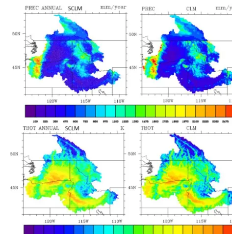
The meteorological forcing in this study was extracted from the phase-two North America Land Data Assimilation Sys-tem (NLDAS-2) at an hourly time step from 1979 to 2008 (Xia et al., 2012), including precipitation, shortwave and long-wave radiation, air temperature, humidity, surface pres-sure and wind speed at 0.125◦ resolution derived from the 32 km resolution 3-hourly North American Regional Reanal-ysis (NARR). For grid-based applications, the NLDAS-2 forcing data are either applied directly at 0.125◦resolution or spatially aggregated to the corresponding coarser resolutions. For SCLM, an area-average algorithm is applied to remap the NLDAS-2 forcing to the subbasins defined by their bound-aries at each spatial resolution. That is, the algorithm com-putes the value of each meteorological variable in a subbasin as the average of the corresponding variable from all the 0.125◦grid cells that intersect with the subbasin weighted by the overlapping areas. ArcGIS is used to link the subbasins to the intersecting grids and to compute the fractional areas of the intersecting grids. Figure 2 shows the spatial distribu-tions of annual mean precipitation and surface temperature of CLM and SCLM in the CRB domain at the finest (0.125◦) resolution. It can be seen from the figure that the differences between the two representations are very small.
Land surface parameters and leaf area index (LAI) are derived from the global land parameter data set developed by Ke et al. (2012) at 0.05◦ resolution based on the most
recent MODIS (Moderate Resolution Imaging Spectrora-diometer) land cover and improved MODIS LAI products. Soil texture is generated based on a hybrid of 30 arcsec State Soil Geographic Database (STATSGO, now referred to as the US General Soil Map) (for CONUS) and 5 min Food and Agriculture Organization (outside CONUS) 16-category two-layer soil-type data (Chen et al., 2007; Miller and White, 1998). The two-layer soil-type data is then converted to com-position of clay and sand (Cosby et al., 1984; Dai et al., 2003) within each 30 arcsec grid cells and interpolated to 10 verti-cal layers down to 3.8 m depth. Soil depth is a notoriously difficult input parameter for hydrology modeling. It is thus greatly simplified in CLM4 by assuming that soil depth has a globally uniform value of 3.8 m (Oleson et al., 2010) in both modeling frameworks. Even though it is a bold assumption, it is typical in the field of land surface modeling due to lack of global soil-depth data. Other land surface parameters such as soil color and soil organic matter are derived from the default 0.5◦CLM4 global input data set provided by NCAR. For the grid-based CLM simulations, the CLM4 preprocessing pack-age (Oleson et al., 2010) is used at each spatial resolution in this study.
The SCLM soil, land cover, and vegetation parameters are derived by overlaying the subbasin boundaries of each spatial
1
Figure 2. Comparison of precipitation and air temperature
repre-sentation in the two modeling frameworks.
resolution over the grids as described above. Similar to the forcing parameters, ArcGIS is used to link the subbasins to the grids and calculate the area weights of the intersect-ing grids. Consistent with the CLM4 preprocessintersect-ing package (Oleson et al., 2010), soil properties such as percent clay, percent sand etc. are calculated using an area-dominant al-gorithm, where each parameter value for the subbasins is as-signed to the value covering the largest fraction of the sub-basin. Land cover characteristics and plant functional types (PFTs) for each subbasin are determined using the area-average algorithm described above for the atmospheric forc-ing. The LAI and stem area index (SAI) parameters for each subbasin are calculated using a PFT-weighted area-average algorithm. Between the two representations, the differences of most land surface parameters are small due to the high res-olution of source data. But this is not the case for soil color since the resolution of source data is 0.5◦, which is much coarser (figure not shown).
(CTIs) are first derived following the definition used in TOP-MODEL (Beven; 1997; Quinn et al., 1995) using ArcGIS. The CTIs are then fitted to a distribution, within each sub-basin or grid, to estimate the topography-relevant hydrologic parameters (i.e.,fmaxandCs). In CLM4 and its previous ver-sions (e.g., CLM3, CLM3.5), these parameters are derived from coarse resolution (e.g., 1 km) DEMs (Niu et al., 2005) due to the lack of higher-resolution DEMs with a global do-main. However, as discussed in our previous study (Li et al., 2011), the estimation of these parameters using 1 km DEMs is problematic due to its inconsistency with hydrology the-ory. Interested readers are referred to Li et al. (2011) for details. With the newly available HydroSHEDS (Lehner et al., 2008) database, 90 m DEM data are now available glob-ally. We therefore estimatedfmaxvalues using the 90 m DEM from HydroSHEDS.
3.4 Methods of analyses
For a fair comparison of the two modeling frameworks, all simulations are driven by the same meteorological forcing (NLDAS-2 1979–2008) and land surface parameters, gen-erated using the same methods described above, and spun up until the state variables such as soil moisture and tem-perature reached equilibrium states. The relative merits of CLM-MOSART and SCLM-MOSART land surface model-ing frameworks in streamflow simulations are then investi-gated using streamflow simulated after the spin up. The two modeling frameworks are compared using two approaches.
In the first comparison, we investigate how the two mod-eling frameworks simulate streamflow across multiple spa-tial scales (defined as the size of upstream drainage area of gauge station) compared to the naturalized streamflow data from the Surface Hydrology Group, University of Washing-ton (http://www.hydro.washingWashing-ton.edu/2860). The sources of differences in simulated streamflow at the highest reso-lution (0.125◦)between the two modeling frameworks are explored in different climatic regions of the CRB and classi-fied based on rainfall/snowfall fractions. The USGS stream gauges are also classified based on the dominant climate regime in their catchment areas for insight on the role of climate in the scalability differences of the modeling works. In the second comparison, the two modeling frame-works are evaluated for their scalability across multiple spa-tial resolutions in both CRB and MW. Scalability is mea-sured by the ability of the models to produce simulations that asymptotically approach the high-resolution simulations as model resolution increases. Model scalability is thus demon-strated by using the simulations performed at 0.125◦ res-olutions (CLM0125-MOSART and SCLM0125-MOSART) as the “reference” solution for comparison with simulations performed at increasingly coarser spatial resolutions.
In both comparisons, we compare the streamflow simu-lated by the two modeling frameworks across multiple spatial scales at the USGS stream gauges selected to represent major
rivers of the CRB. Absolute differences in specific peak flows (ADP) (long-term average peak streamflow normalized by the corresponding contributing area) are calculated at all the stream gauges of the CRB and selected using the procedure described in Sect. 3.2 between each coarse-resolution simu-lation and the corresponding finest-resolution (0.125◦) sim-ulation. The ADP values are used to evaluate the scalability of the two modeling frameworks in simulating peak flow at multiple temporal scales. Furthermore, Nash–Sutcliffe effi-ciency (NSE) values are calculated at the same stream gauges between the streamflows simulated by each coarse resolution and the corresponding reference (finest resolution) simula-tion as shown below:
NSE=1− 6(Fr−Fc)
2
6(Fr−Frave)2
, (1)
where,Fr,Fc, andFraveare streamflow simulated by the ref-erence simulation, coarse-resolution simulation, and average streamflow from the reference solution, respectively. To un-derstand the role of contributing area on model scalability, the NSE values are also calculated using streamflow values normalized by the respective contributing area. A nonpara-metric statistical significance test is employed using the CRB stream gauges to evaluate the significance of the scalabil-ity differences between the two modeling frameworks. Fi-nally, NSE values are calculated at the USGS stream gauges of the MW domain that are selected based on the proce-dure described in Sect. 3.2 (Fig. 1) to investigate scalabil-ity of the two modeling frameworks at the spatial resolutions that showed statistically significant differences in scalability in the CRB study domain. The comparison at the MW do-main is further extended to the MW dodo-main basins (MSRB, UMRB and OHRB, respectively, Missouri, Upper Missis-sippi and Ohio river basins) to gain more insight on any dif-ferences at a regional scale. Results from these analyses are discussed in the following section.
4 Simulation results and analysis
4.1 Runoff and streamflow at the finest spatial resolution
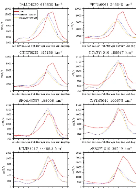
1 Figure 3. Streamflow from the finest SMOSART and
CLM-MOSART compared to naturalized flow (Qobs) across different spatial scales.
naturalized streamflow, both SMOSART and CLM-MOSART underestimate streamflow in the northern part of the CRB (as indicated by the comparison at the ARROW, CHIEF and PRIRA stream gauges) and overestimate stream-flow in the southern part (as indicated by the comparison at the MILNE, BROWN and HCANY stream gauges). Since the northern part is wetter and provides more runoff than the southern part (e.g., streamflow at CHIEF is much higher than HCANY although they have comparable drainage area), both SCLM-MOSART and CLM-MOSART slightly under-estimate streamflow at the DALLE stream gauge, which is downstream of the confluence where the two parts join each other. Also, at most stream gauges, both SCLM-MOSART and CLM-MOSART produce peak flow 1 month earlier than the naturalized streamflow. This can be attributed to the pa-rameterization of snow processes in CLM that very often leads to earlier snowmelt (Wang et al., 2008; Li et al., 2011). Due to the earlier snowmelt, one may conclude that SCLM-MOSART does not necessarily perform better than CLM-MOSART in simulating streamflow. One reason why SMOSART is not performing better than CLM-MOSART is that the runoff simulations in SCLM and CLM
are both governed by the same set of hydrological formula-tions and parameters originally calibrated for CLM based on the grid-based configuration at the global scale. If reproduc-ing the observed streamflow is the target, a fair comparison between SCLM-MOSART and CLM-MOSART should be conducted with separate parameter calibration for each. The effective and meaningful parameter calibration of SCLM and CLM, however, is itself challenging particularly over large regions. This has been a topic of research in separate stud-ies (Huang et al., 2013; Sun et al., 2013), and is beyond the scope of this study. Here, our main objective is to investi-gate the differences between the two modeling frameworks in streamflow simulation caused purely by different approaches to delineating the fundamental spatial units without changes in model parameters or adjustments of model parameteriza-tions to take advantage of one representation over the other.
Streamflow is a direct product of runoff routing processes that are fed by, and therefore directly controlled by, runoff generation in terms of both magnitude and timing. Runoff generation itself is controlled by the interactions between cli-mate and landscape properties and the latter two are very of-ten closely interrelated to each other. Thus, to explain the differences in streamflow simulation between the two mod-eling frameworks, we first explore their differences in sim-ulating runoff generation in different climate regimes. For this purpose, the subbasins/grids of the finest (0.125◦) reso-lution in the CRB domain are grouped into different regimes by rainfall fraction (ratio of rainfall to the total precipitation) as snow dominated (areas with rainfall fraction ranging be-tween 0.1 and 0.5), intermediate (areas with rainfall fraction ranging between 0.5 and 0.75), and rain dominated (areas with rainfall fraction ranging between 0.75 and 1.0) regimes (Fig. 4). The grids and subbasins are classified based on the same criteria, which result in spatial distributions of rainfall fraction largely consistent with the spatial distribution of el-evation in the basin in both representations. This is not sur-prising since rainfall/snowfall partitioning of precipitation is dominated by near-surface air temperature, which is closely related to elevation variation (Tesfa et al., 2014). The total area of each regime in the CRB is listed in Table 1. Using different thresholds of 0.1, 0.4, 0.7 and 1.0 does not change the conclusions except the snow-dominated area is rather small as the two middle thresholds decrease. Hence subse-quent analysis is based on the classification with thresholds of 0.1, 0.5, 0.75, and 1.0. In the subsequent sections, the cli-mate regimes are used to investigate the differences of the two modeling frameworks in runoff generation.
1 Figure 4. Climate regions based on model simulated
rain-fall/snowfall partitioning.
Table 1. The portion of areas within three climate regimes (km2).
SCLM CLM
Snow-dominated 71 064 87 756 Rain–snow mixing 254 267 223 440 Rain-dominated 327 687 340 240
Total 653 018 651 437
the snow-dominated areas, SCLM-MOSART produces less subsurface runoff due to drier soil (Fig. 5). The latter is be-cause the evaporation from bare soil and canopy simulated by SCLM-MOSART is overall slightly higher than that sim-ulated by CLM-MOSART, which affect the soil moisture simulations. Compared to the phase shift in the simulated streamflow shown in Fig. 3, the phase shift in the simu-lated runoff is less significant. However, the transformation from runoff to streamflow is captured by the routing pro-cess, which is nonlinear in nature. Therefore one could infer that it is this transformation that has amplified the phase dif-ference between the runoff simulated by the two modeling frameworks. It is then logical to ask whether and how this phase difference exists in the climatic forcings that are major drivers of runoff generation processes.
Figure 6 shows the seasonal variation of precipitation, temperature, and the partitioning of precipitation into rain-fall and snowrain-fall in the two modeling frameworks. From the plots for the whole CRB, one can see that there is no dif-ference between the mean precipitation and temperature av-eraged over all subbasins and grids, which is expected be-cause the remapping from grids to subbasins conserves the area-averaged forcings used as inputs to the models. How-ever, the total precipitation is noticeably larger in CLM than SCLM in the snow-dominated areas, which is compensated by slightly smaller precipitation in CLM than SCLM in the rain-dominated areas, as the latter occupies a much larger fraction of the total area of the CRB. Similarly, the differ-ences in rainfall and snowfall are more noticeable in the snow-dominated areas, with smaller differences in rainfall also noted in the rain-dominated areas. The models partition the total precipitation into rainfall/snowfall depending on air
1 Figure 5. Seasonality of runoff and soil water over the climate
re-gions. Note that soil water is included here because it is closely related to the runoff generation.
temperature. From the plots of air temperature for the differ-ent regimes, the difference between the two modeling frame-works is barely discernible in any climate regime. However, even very small differences in air temperature can lead to no-ticeable differences in the partitioning of rainfall/snowfall in areas with very high total precipitation. Hence larger total precipitation in CLM in the snow-dominated areas translates to larger snowfall in the cold season and larger rainfall in the warm season compared to SCLM, with opposite compen-sating effects in the rain-dominated areas. These differences reflect the dominant control of topography, hence air tem-perature, on the precipitation regimes; therefore, the model’s spatial structure has an impact on precipitation regimes that translate to differences in runoff (Fig. 5) and streamflow (Fig. 3) due to the runoff generation and river routing pro-cesses.
4.2 Scalability of streamflow simulations
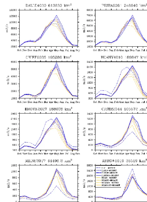
In this analysis, we explore how the two modeling frame-works simulate streamflow at different spatial resolutions. Figure 7 compares the streamflow simulated by SCLM-MOSART and CLM-SCLM-MOSART at all spatial resolutions (0.125◦, 0.25◦, 0.5◦, and 1◦) at the USGS stream gauges
1
Figure 6. Seasonality of forcing over the climate regions.
1◦resolution. This is particularly true over smaller drainage areas such as manifested at the HCANY, BROWN, CJSTR, MILNE and ARROW stream gauges. This issue is thus in-vestigated further at the stream gauges selected in Sect. 3.2 in the subsequent sections.
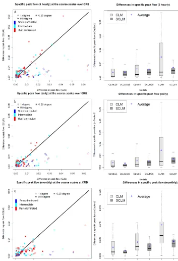
Shown in Fig. 8 are scatterplots and statistics boxplots of the absolute differences in specific peak flow (ADP) cal-culated, as described in Sect. 3.4, between each coarse-resolution simulation and the corresponding reference sim-ulation at 0.125◦resolution in each modeling framework at
3-hourly (Fig. 8a, d), daily (Fig. 8b, e) and monthly (Fig. 8c, f) timescales. In the figure, symbols represent spatial reso-lutions, while colors are used to identify the dominant cli-mate regimes in the catchment area of the stream gauges. From the scatterplots, it is obvious that the differences be-tween the coarse simulations and the reference simulation from SCLM are generally smaller than that from CLM, es-pecially in snow-dominated areas (e.g., the blue symbols are more often below the 1 : 1 line than the red symbols), consis-tent with the finding of Tesfa et al. (2014) for runoff. Hence in both types of plots (scatterplots and boxplots), SCLM-MOSART tends to show some scalability advantages com-pared to CLM-MOSART at all temporal scales, which be-comes more evident as one goes from 3-hourly to monthly temporal scales, particularly at the 0.5◦ and 1◦ resolutions.
In general, these results suggest that improved scalability in runoff generation combined with the routing processes re-sulted in better scalability in peak flow simulation for SCLM-MOSART compared to CLM-SCLM-MOSART at the stream gauges within the CRB domain.
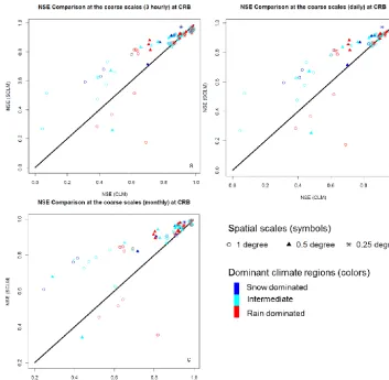
We also calculated NSE values between each coarse-resolution simulation and the reference simulation to com-pare scalability of the two approaches. Figure 9 comcom-pares the NSE values of the two modeling frameworks calculated
1 Figure 7. Streamflow from different resolution SCLM-MOSART
and CLM-MOSART simulations across different spatial scales (drainage area).
for each coarse resolution (0.25◦, 0.5◦, and 1◦) at the
1 Figure 8. Specific peak flow comparison at 3-hourly, daily and monthly temporal scales at the USGS stations with contributing area larger
than 15 000 km2: (a), (b) and (c) comparison over the climate regions and (d), (e) and (f) comparing their statistics.
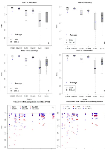
As streamflow simulated at the stream gauges depends on the contributing areas, it is important to determine if con-tributing area differences between the two approaches may play a role in the scalability differences and how scalabil-ity differences may vary across spatial scales (i.e., upstream drainage areas of the stream gauges). We calculated another set of NSE values by normalizing the simulated streamflow
1
Figure 9. Scalability comparison using a NSE of streamflow at 3-hourly (a), daily (b) and monthly (c) calculated between each coarse scale
and the corresponding fine scale in each modeling framework at the USGS stations with contributing area larger than 15 000 km2.
in streamflow simulation. Results also show more clearly that the scalability advantages of SCLM-MOSART are more sig-nificant at the 0.5◦ and 1◦ spatial resolutions. Comparison
of the two sets of NSEs across spatial scales shows that the slight differences between the area normalized (Fig. 10c) and nonnormalized (Fig. 10f) streamflow occur mostly at stream gauges with smaller drainage areas (less than ∼105km2), suggesting that the role of contributing area on the scala-bility differences of the two modeling frameworks dimin-ishes as the spatial scale increases. The results also show that both modeling frameworks have a threshold behav-ior with increasing spatial scale (drainage area), that is, in both sets of NSE values, the ability to reproduce the finest-resolution (0.125◦) simulations generally improve with in-creasing catchment size at all spatial resolutions (0.25◦, 0.5◦, and 1◦). But, in both sets of NSE values, SCLM-MOSART results converge to the reference simulation faster with in-creasing drainage areas than that of CLM-MOSART at all coarse spatial resolutions. Comparisons at 3-hourly and daily temporal scales show the same pattern (figures not shown).
Following the results discussed so far, it is logical to ask whether the scalability advantages of SCLM-MOSART have any statistical significance. Table 2 shows thepvalue results from a nonparametric statistical significance t test (Bauer, 1972) on the NSEs calculated from the nonnormal-ized streamflow at each coarse (0.25◦, 0.5◦, and 1◦) spatial resolution at 3-hourly, daily and monthly temporal scales. Using a confidence level of 95 %, the results show (1) sig-nificant differences in NSEs between SCLM-MOSART and CLM-MOSART at the 0.5◦ and 1◦ spatial resolutions at all (3-hourly, daily and monthly) temporal scales, (2) insignif-icant difference in NSEs at 0.25◦ resolution at all temporal scales, and (3) the significance of the differences in NSEs be-tween the two modeling frameworks increases from 3-hourly to monthly temporal scales.
1 Figure 10. Statistics of (a and b) area-normalized and (d and e) nonnormalized NSEs of streamflow at different temporal scales and (c and f) NSEs of monthly streamflow across the spatial scale over USGS stations with drainage area greater than 15 000 km2in the CRB.
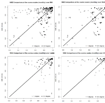
resolutions that showed statistically significant scalability differences in the CRB domain. For this purpose, NSE values are calculated using the nonnormalized streamflow simulated at the coarse (0.5◦ and 1◦) resolutions and the correspond-ing reference (0.125◦resolution). Figure 11a shows minimal scalability differences between the two frameworks in MW. Since the MW domain is large and more heterogeneous in climate and topographic regimes than the CRB, we further
1
Figure 11. NSE values from monthly streamflow compared at the USGS stations with contributing area larger than 15 000 km2located in the whole Midwest (a), and Missouri (b), Upper Mississippi (c) and Ohio (d) regions.
Table 2. Nonparametrict-testpvalues on NSE.
Spatial Scale
Temporal scale 0.25◦ 0.5◦ 1◦
3-hourly 0.9972 5.583×10⁻⁴ 9.0751×10⁻³
Daily 0.9964 3.670×10⁻⁴ 8.5951×10⁻³
Monthly 7.699×10⁻² 3.724×10⁻⁷ 2.133×10⁻³
and the CRB domains, the results at the whole MW domain, MSRB, as well as UMRB are not surprising. The MW do-main is dominated by flat topography and precipitation oc-curs mainly as rain, while the CRB domain is dominated by mountainous topography and precipitation occurs mainly as snow. Thus, these results are generally consistent with the findings in Tesfa et al. (2014), which showed the scalabil-ity advantages of the subbasin-based land surface modeling in runoff generation to be dominated by its superior scala-bility in mountainous and snow-dominated regions due to better consistency in representing mountainous topography
and snow over complex topographic regions. However, the results over OHRB deserve further investigation.
1
Figure 12. Topographic slope and rainfall fraction over the Missouri, Upper Mississippi and Ohio regions.the scalability of the rain driven saturated component of sur-face runoff. These results thus generally suggest that the scal-ability differences in streamflow simulation between the two modeling frameworks are generalizable to other regions.
5 Summary and conclusions
In this study, we have implemented a subbasin-based rep-resentation of CLM called SCLM, coupled with a physi-cally based river routing model (MOSART). The relative merits of the subbasin-based modeling framework (SCLM-MOSART) in streamflow simulation are compared to the grid-based modeling framework (CLM-MOSART) over to-pographically and climatologically contrasting regions: the Columbia River Basin (CRB) and US Midwest region (MW). For this purpose, the two modeling frameworks are ap-plied at four spatial resolutions (0.125◦, 0.25◦, 0.5◦, and 1◦) in both the CRB and MW, and streamflow simulated by SCLM-MOSART and CLM-MOSART are compared with each other and with naturalized streamflow data.
We found that in the CRB where topography dominantly controls the precipitation regimes, small differences be-tween the averaged atmospheric forcing for the two mod-eling frameworks could lead to larger differences in simu-lated runoff and streamflow at the finest (0.125◦) resolution because of the nonlinear runoff generation and streamflow routing processes. Our results showed that simply by using a spatial structure that follows subbasin boundaries defined by topography without any change in model parameteriza-tions, SCLM-MOSART exhibits improved scalability in sim-ulating both peak and mean streamflow compared to CLM-MOSART. The scalability advantages of SCLM-MOSART are more apparent in snow-dominated and intermediate cli-mate regimes, and in areas with steeper topography. This suggests that the scalability advantages of SCLM in runoff generation, discussed in Tesfa et al. (2014), are preserved
even after coupling with the routing model (MOSART). Both modeling frameworks showed a threshold behavior with spatial scales (drainage area of the stream gauges); i.e., for drainage area larger than a threshold, spatial reso-lution becomes less important so the coarse-resoreso-lution simu-lations resemble the fine-resolution simusimu-lations, but SCLM-MOSART converges to the high-resolution simulations faster with increasing drainage area than CLM-MOSART. Lastly, we found that the understanding on scalability differences in streamflow simulation between the two modeling frame-works is generalizable to other regions.
The scalability results presented in this study suggest that the subbasin-based representation is more robust than the grid-based representation across spatial scales. This reduced sensitivity to model resolution for both peak and mean flow is an important advantage for reliable hydrologic predictions. Given that the scalability advantages have been identified for both runoff generation and streamflow simulations, it would be valuable to further examine how the scalability advantages partition between the two nonlinear processes and further contrast scalability differences in different topographic and climate regions. This would include (1) analyses of runoff generation over the catchment area of each stream gauge; and (2) a detailed investigation of river routing parameters such as drainage density, topographic slope and channel ge-ometry, which are potential sources of differences between the streamflow simulated by the two modeling frameworks. Furthermore, given that the topography-relevant runoff gen-eration parameter,fmax, is derived from the HydroSHEDS (Lehner et al., 2008) 90 m DEM database, which is at a con-siderably finer resolution compared to the 1 km data provided with CLM4, it would be valuable to examine its relative mer-its on runoff generation/streamflow simulation in the two modeling frameworks across different spatial resolutions.
in CLM4, assuming a globally uniform soil-depth value of 3.8 m (Oleson et al., 2010). Even though it is a bold assump-tion, it is typical in the field of land surface modeling due to lack of global soil-depth data. Effective incorporation of spatially distributed soil depth in CLM requires two major steps: (1) deriving a large-scale soil-depth map; and (2) sig-nificant modifications of CLM source code to accommodate new soil-layer delineation and associated hydrology, ther-modynamics and biogeochemical processes. Both of these steps demand substantial efforts and cannot be achieved in a short period. We therefore leave the soil-depth issue for fu-ture study.
The analyses presented in this study, covering a wide range of model resolutions, are particularly useful as the land sur-face modeling community is exploring the feasibility and ad-vantages of ultra-high resolution (e.g., 1 km resolution glob-ally) (Wood et al., 2011). Conceptually, the differences be-tween the two approaches may be larger as lateral water redistribution becomes increasingly important in determin-ing soil moisture states at smaller spatial scales. The results in this study also suggest that without proper calibration, SCLM-MOSART may not necessarily perform better than CLM-MOSART. A fair comparison between the two model-ing frameworks in reproducmodel-ing the observed streamflow re-quires a separate proper parameter calibration for each; thus, future research to include parameter calibration of SCLM and CLM on smaller basins with good forcing and evalua-tion data would be useful to test this point. Given that CLM is the land component of an Earth system model and can interact with the atmosphere component and ocean compo-nent, it would be valuable to examine how the subbasin-based representation of terrestrial processes may affect the global cycling of water and energy between land, atmosphere and ocean. Such a scientific pursuit is now supported by re-cent progresses made in software engineering. With the lat-est public versions of the Community Climate System model and the Community Earth System model (i.e., CCSM4 and CESM1) there is a suite of new coupling capabilities in the CPL7 coupler that allow more flexibility and extensibility for very-high-resolution modeling and coupling Earth sys-tem components configured on unstructured grids (Craig et al., 2012).
Acknowledgements. This study is supported by the Office of
Science of the US Department of Energy as part of the Earth System Modeling and the Integrated Assessment Research pro-grams. The PNNL Platform for Regional Integrated Modeling and Analysis (PRIMA) initiative supported the development of various data sets and applications of the models to perform the numerical experiments. The Pacific Northwest National Laboratory is operated by Battelle for the US Department of Energy under Contract DE-AC06-76RLO1830.
Edited by: J. Neal
References
Bauer, D. F.: Constructing confidence sets using rank statistics, J. Am. Stat. Assoc., 67, 687–690, 1972.
Beven, K.: TOPMODEL: A critique, Hydrol. Process., 11, 1069– 1085, 1997.
Bloschl, G. and Sivapalan, M.: Scale Issues in Hydrological Mod-eling – a Review, Hydrol. Process., 9, 251–290, 1995.
Boone, A., Habets, F., Noilhan, J., Clark, D., Dirmeyer, P., Fox, S., Gusev, Y., Haddeland, I., Koster, R., Lohmann, D., Ma-hanama, S., Mitchell, K., Nasonova, O., Niu, G.-Y., Pitman, A., Polcher, J., Shmakin, A. B., Tanaka, K., Van Den Hurk, B., Ver-ant, S., Verseghy, D., Viterbo, P., and Yang, Z.-L.: The Rhône-Aggregation Land Surface Scheme Intercomparison Project: An Overview, J. Climate, 17, 187–208, doi:10.1175/1520-0442(2004)017<0187:TRLSSI>2.0.CO;2, 2004.
Bruneau, P., Gascuel-Odoux, C., Robin, P., Merot, P., and Beven, K.: Sensitivity to Space and Time Resolution of a Hydrological Model Using Digital elevation Data, Hydrol. Process., 9, 69–81, 1995.
Cerdan, O., Le Bissonnais, Y., Govers, G., Lecomte, V., van Oost, K., Couturier, A., King, C., and Dubreuil, N.: Scale effect on runoff from experimental plots to catchments in agricultural areas in Normandy, J. Hydrol., 299, 4–14, doi:10.1016/j.jhydrol.2004.02.017, 2004.
Chen, F. and Avissar, R.: Impact of land-surface moisture variabil-ities on local shallow convective cumulus and precipitation in large-scale models, J. Appl. Meteorol., 33, 1381–1394, 1994. Chen, F., Manning, K., LeMone, M. A., Trier, S. B., Alfieri, J. G.,
Roberts, R., Tewari, M., Niyogi, D., Horst, T., and Oncley, S. P.: Description and evaluation of the characteristics of the NCAR high-resolution land data assimilation system, J. Appl. Meteorol. Clim., 46, 694–713, 2007.
Cosby, B. J., Hornberger, G. M., Clapp, R. B., and Ginn, T. R.: A Statistical Exploration of the Relationships of Soil Moisture Characteristics to the Physical Properties of Soils, Water Resour. Res., 20, 682–690, 1984.
Craig, A. P., Vertenstein, M., Jacob, R.: A new flexible coupler for earth system modeling developed for CCSM4 and CESM1, Comput. Appl., 26, 31–42, doi:10.1177/1094342011428141, 2012.
Dai, Y. J., Zeng, X., Dickinson, R., Baker, I., Bonan, G., Bosilovich, M., Denning, S., Dirmeyer, P., Houser, P., Niu, G., Oleson, K., Schlosser, A., and Yang, Z.-L.: The Common Land Model, B. Am. Meteorol. Soc., 84, 1013–1023, 2003.
Famiglietti, J. S. and Wood, E. F.: Mutiscale modeling of spa-tially variable water and energy balances, Water Resour. Res., 30, 3061–3078, 1994.
Goteti, G., Famiglietti, J. S., and Asante, K.: A Catchment-Based Hydrologic and Routing Modeling System with explicit river channels, J. Geophys. Res., 113, D14116, doi:10.1029/2007JD009691, 2008.
Guo, J., Liang, X., and Leung, L. R.: A new multi-scale flow net-work generation scheme for land surface models, Geophys. Res. Lett., 31, L23502, doi:10.1029/2004GL021381, 2004.
Hou, Z., Huang, M., Leung, L. R., Lin, G., and Ricciuto, D. M.: Sensitivity of surface flux simulations to hydrologic parame-ters based on an uncertainty quantification framework applied to the Community Land Model, J. Geophys. Res., 117, D15108, doi:10.1029/2012JD017521, 2012.
Huang, M. and Liang, X.: On the assessment of the impact of re-ducing parameters and identification of parameter uncertainties for a hydrologic model with applications to ungauged basins, J. Hydrol., 320, 37–61, 2006.
Huang, M., Xu, L., and Leung, L. R.: A Generalized Subsurface Flow Parameterization Considering Subgrid Spatial Variability of Recharge and Topography, J. Hydrometeorol., 9, 1151–1171, 2008.
Huang, M., Hou, Z., Leung, L. Y. R., Ke, Y., Liu, Y., Fang, Z., and Sun, Y.: Uncertainty Analysis of Runoff Simulations and Parameter Identifiability in the Community Land Model – Evi-dence from MOPEX Basins, J. Hydrometeorol., 14, 1754–1772, doi:10.1175/JHM-D-12-0138.1, 2013.
Ke, Y., Leung, L. R., Huang, M., Coleman, A. M., Li, H., and Wig-mosta, M. S.: Development of high resolution land surface pa-rameters for the Community Land Model, Geosci. Model Dev., 5, 1341–1362, doi:10.5194/gmd-5-1341-2012, 2012.
Kirkby, M. J.: From Plot to Continent: Reconciling Fine and Coarse Scale Erosion Models, in: Sustaining the Global Farm, Selected papers from the 10th International Soil Conservation Organiza-tion Meeting held May 24–29, 1999, edited by: Scott, D. E., Mo-htar, R. H., and Steinhardt, G. C., 860–870, Purdue University and the USDA-ARS National Soil Erosion Research Laboratory, 2001.
Koren, V. I., Finnerty, B. D., Schaake, J. C., Smith, M. B., Seo, D. J., and Duan, Q. Y.: Scale dependencies of hydrologic models to spatial variability of precipitation, J. Hydrol., 217, 285–302, doi:10.1016/S0022-1694(98)00231-5, 1999.
Koster, R. D., Suarez, M. J., Ducharne, A., Stieglitz, M., and Ku-mar, P.: A catchment-based approach to modeling land surface processes in a GCM: 1. Model structure, J. Geophys. Res., 105, 24809–24822, 2000.
Lawrence, D., Oleson, K. W., Flanner, M. G., Thorton, P. E., Swenson, S. C., Lawrence, P. J., Zeng, X., Yang, Z. L., Levis, S., and Skaguchi, K.: Parameterization improvements and func-tional and structural advances in version 4 of the Commu-nity Land Model, J. Adv. Model. Earth Syst., 3, M03001, doi:10.1029/2011MS000045, 2011.
Lawrence, P. J. and Chase, T. N.: Representing a new MODIS con-sistent land surface in the Community Land Model (CLM 3.0), J. Geophys. Res., 112, G01023, doi:10.1029/2006JG000168, 2007. Lehner, B., Verdin, K., and Jarvis, A.: New global hydrograhy de-rived from spaceborne elevation data, Eos T. Am. Geophys. Un., 89, 93–94, 2008.
Leung, L. R. and Ghan, S. J.: A subgrid parameterization of oro-graphic precipitation, Theor. Appl. Climatol., 52, 95–118, 1995. Leung, L. R. and Ghan, S. J.: Parameterizing subgrid orographic precipitation and surface cover in climate models, Mon. Weather Rev., 126, 3271–3291, 1998.
Li, H., Huang, M., Wigmosta, M. S., Ke, Y., Coleman, A. M., Le-ung, L. R., Wang, A., and Ricciuto, D. M.: Evaluating runoff simulations from the Community Land Model 4.0 using observa-tions from flux towers and a mountainous watershed, J. Geophys. Res., 116, D24120, doi:10.1029/2011JD016276, 2011.
Li, H., Wigmosta, M. S., Wu, H., Huang, M., Ke, Y., Coleman, A. M., and Leung, L. R.: A physically based runoff routing model for land surface and earth system models, J. Hydrometeorol., 14, 808–828, doi:10.1175/JHM-D-12-015.1, 2013.
Liang, X., Wood, E. F., and Lettenmaier, D. P.: Surface soil moisture parameterization of the VIC-2L model: Evaluation and modifica-tions, Global Planet. Change, 13, 195–206, 1996.
Liang, X., Guo, J., and Leung, L. R.: Assessment of the effects of spatial resolutions on daily water flux simulations, J. Hydrol., 298, 287–310, doi:10.1016/j.jhydrol.2003.07.007, 2004. Miller, D. A. and White, R. A.: A Conterminous United States
Mul-tilayer Soil Characteristics Dataset for Regional Climate and Hy-drology Modeling, Earth Interact., 2, 1–26, 1998.
Neitsch, S. L., Arnold, J. G., Kiniry, J. R., Srinivasan, R., and Williams, J. R.: Soil and Water Assessment Tool Theoreti-cal Documentation, version 2005, Temple, TX: Grassland, Soil and Water Research Laboratory, Agricultural Research Service, available at: http://swatmodel.tamu.edu/documentation (last ac-cess: March 2013), 2005.
Niu, G.-Y. and Yang, Z.-L.: Effects of frozen soil on snowmelt runoff and soil water storage at a continental scale, J. Hydrome-teorol., 7, 937–952, doi:10.1175/JHM538.1, 2006.
Niu, G.-Y., Yang, Z.-L., Dickinson, R. E., and Gulden, L. E.: A simple TOPMODEL-based runoff parameterization (SIMTOP) for use in global climate models, J. Geophys. Res., 110, D21106, doi:10.1029/2005JD006111, 2005.
Oleson, K. W., Lawrence, D. M., Bonan, G. B., Flanner, M. G., Kluzek, E., Lawrence, P. J., Levis, S., Swenson, S. C., and Thornto, P. E.: Technical Description of version 4.0 of the Com-munity Land Model (CLM), 257 pp., National Center for Atmo-spheric Research, Boulder, 2010.
Pielke, RA Sr.: Influence of the spatial distribution of vegetation and soils on the prediction of cumulus convective rainfall, Rev. Geophys., 39, 151–177, 2001.
Quinn, P., Beven, K., Culf, A.: The introduction of macroscale hydrological complexity into land surface–atmosphere transfer models and the effect on the planetary boundary layer develop-ment, J. Hydrol., 166, 421–444, 1995.
Schulze, R.: Transcending scales of space and time in impact stud-ies of climate and climate change on agrohydrological responses, Agr. Ecosyst. Environ., 82, 185–212, doi:10.1016/S0167-8809(00)00226-7, 2000.
Shrestha, R., Tachikawa, Y., and Takara, K.: Input data resolution analysis for distributed hydrological modeling, J. Hydrol., 319, 36–50, 2006.
Sivapalan, M. and Kalma, J. D.: Scale Problems in Hydrology – Contributions of the Robertson Workshop, Hydrol. Process, 9, 243–250, 1995.
Sridhar, V., Elliott, R. L., and Chen, F.: Scaling effects on modeled surface energy-balance components using the NOAH-OSU land surface model, J. Hydrol., 280, 105–123, doi:10.1016/S0022-1694(03)00220-8, 2003.
Sun, Y., Hou, Z., Huang, M., Tian, F., and Ruby Leung, L.: Inverse modeling of hydrologic parameters using surface flux and runoff observations in the Community Land Model, Hydrol. Earth Syst. Sci., 17, 4995–5011, doi:10.5194/hess-17-4995-2013, 2013. Tesfa, T. K., Tarboton, D. G., Chandler, D. G., and McNamara, J. P.:
Water Resour. Res. 45, W10438, doi:10.1029/2008WR007474, 2009.
Tesfa, T. K., Leung, L.-Y. R., Huang, M., Li, H., Voisin, N., Wigmosta, M. S.: Scalability of grid- and subbasin-based land surface modeling approaches for hydrologic simulations, J. Geophys. Res.-Atmos., 119, 3166–3184, doi:10.1002/2013JD020493, 2014.
Wang, A., Li, K. Y., and Lettenmaier, D. P.: Integration of the variable infiltration capacity model soil hydrology scheme into the community land model, J. Geophys. Res., 113, D09111, doi:10.1029/2007JD009246, 2008.
Wen, Z., Liang, X., and Yang, S.: A new multiscale routing frame-work and its evaluation for land surface modeling applications, Water Resour. Res., 48, W08528, doi:10.1029/2011WR011337, 2012.
Wolock, D. M. and Price, C. V.: Effects of digital eleva-tion model map scale and data resolueleva-tion on a topography-based watershed model, Water Resour. Res., 30, 3041–3052, doi:10.1029/94WR01971, 1994.
Wood, E. F., Sivapalan, M., Beven, K., and Band, L.: Effects of spa-tial variability and scale with implications to hydrologic model-ing, J. Hydrol., 102, 29–47, 1988.
Wood, E. F., Roundy, J. K., Troy, T. J., van Beek, L. P. H., Bierkens, M. F. P., Blyth, E., de Roo, A., Döll, P., Ek, M., Famiglietti, J., Gochis, D., van de Giesen, N., Houser, P., Jaffé, P. R., Kol-let, S., Lehner, B., Lettenmaier, D. P., Peters-Lidard, C., Siva-palan, M., Sheffield, J., Wade, A., and Whitehead, P.: Hyperres-olution global land surface modeling: Meeting a grand challenge for monitoring Earth’s terrestrial water, Water Resour. Res., 47, W05301, doi:10.1029/2010WR010090, 2011.
Woods, R., Sivapalan, M., and Duncan, M.: Investigating the Rep-resentative Elementary Area Concept – an Approach Based on Field Data, Hydrol. Process., 9, 291–312, 1995.
Wu, H., Kimball, J. S., Mantua, N., and Stanford, J.: Automated up-scaling of river networks for macroscale hydrological modeling. Water Resour. Res., 47, W03517, doi:10.1029/2009WR008871, 2011.
Wu, H., Kimball, J. S., Li, H., Huang, M., Leung, L. R., and Adler, R. F.: A New Global River Network Database for Macroscale Hydrologic modeling, Water Resour. Res., 48, W09701, doi:10.1029/2012WR012313, 2012.