Estimating soil organic carbon stocks of Swiss forest soils by robust external-drift kriging

(1)

www.geosci-model-dev.net/7/1197/2014/ doi:10.5194/gmd-7-1197-2014

Estimating soil organic carbon stocks of Swiss forest soils by robust

external-drift kriging

M. Nussbaum1, A. Papritz1, A. Baltensweiler2, and L. Walthert2

1_{Institute of Terrestrial Ecosystems (ITES), ETH Zurich, Universitätstrasse 16, 8092 Zürich, Switzerland} 2_{Swiss Federal Institute for Forest, Snow and Landscape Research (WSL), Zürcherstrasse 111,}

8903 Birmensdorf, Switzerland

Correspondence to: M. Nussbaum (madlene.nussbaum@env.ethz.ch)

Received: 11 November 2013 – Published in Geosci. Model Dev. Discuss.: 23 December 2013 Revised: 15 April 2014 – Accepted: 19 May 2014 – Published: 25 June 2014

Abstract. Accurate estimates of soil organic carbon (SOC) stocks are required to quantify carbon sources and sinks caused by land use change at national scale. This study presents a novel robust kriging method to precisely estimate regional and national mean SOC stocks, along with truthful standard errors. We used this new approach to estimate mean forest SOC stock for Switzerland and for its five main ecore-gions.

Using data of 1033 forest soil profiles, we modelled stocks of two compartments (0–30, 0–100 cm depth) of mineral soils. Log-normal regression models that accounted for cor-relation between SOC stocks and environmental covariates and residual (spatial) auto-correlation were fitted by a newly developed robust restricted maximum likelihood method, which is insensitive to outliers in the data.

Precipitation, near-infrared reflectance, topographic and aggregated information of a soil and a geotechnical map were retained in the models. Both models showed weak but signif-icant residual autocorrelation. The predictive power of the fitted models, evaluated by comparing predictions with in-dependent data of 175 soil profiles, was moderate (robust R2=0.34 for SOC stock in 0–30 cm andR2=0.40 in 0– 100 cm). Prediction standard errors (SE), validated by com-paring point prediction intervals with data, proved to be con-servative.

Using the fitted models, we mapped forest SOC stock by robust external-drift point kriging at high resolution across Switzerland. Predicted mean stocks in 0–30 and 0– 100 cm depth were equal to 7.99 kg m−2 (SE 0.15 kg m−2) and 12.58 kg m−2 (SE 0.24 kg m−2), respectively. Hence, topsoils store about 64 % of SOC stocks down to 100 cm

depth. Previous studies underestimated SOC stocks of top-soil slightly and those of subtop-soils strongly. The comparison further revealed that our estimates have substantially smaller SE than previous estimates.

1 Introduction

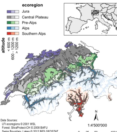
Greenhouse gas (GHG) reporting for the sector “LULUCF – Land Use, Land-Use Change and Forestry” of the United Na-tions Framework Convention on Climate Change and the Ky-oto PrKy-otocol requires national estimates of soil organic car-bon (SOC) stock. SOC stock estimates are needed as baseline and for quantifying carbon (C) sources and sinks caused by land use change. Switzerland, as an example, uses a Tier-2 approach (IPCC, 2003) for SOC stock changes due to con-version between settlements, wetlands, forest-, crop-, grass-land and other grass-land cover types (FOEN, 2012a). Respective estimates are reported for the five ecoregions Jura, Central Plateau, Pre-Alps, Alps and Southern Alps and for the entire country (Fig. 1, Brassel and Lischke, 2001).

(2)

0 25 50 100km

±

Data Sources:

1:4'500'000

ecoregion

al

tit

ud

e

<

60

0

m

60

0

- 1

20

0

m

>

12

00

m

Jura

Central Plateau Pre-Alps Alps Southern Alps

Figure 1. Ecoregions of Switzerland, stratified by altitudinal class.

Hence, CM capitalises on benefits of spatial stratification, but Perruchoud et al. (2000) demonstrated that respective gains may be small.

Perruchoud et al. (2000) and other authors (e.g. Leifeld et al., 2005; Meersmans et al., 2008, 2011, 2012a) used lin-ear models (LM) to relate SOC to covariates characterising soil formation by climate, vegetation, topography, geology and land management. More recently, Grimm et al. (2008), Martin et al. (2011) and Wiesmeier et al. (2011) used non-linear machine learning (ML) methods to the same end. Such statistical modelling of SOC needs covariates that are avail-able contiguously in space because mean stocks are esti-mated by averaging point predictions done by LM or ML for the nodes of a fine-meshed grid over a region of interest, which is equivalent to a discrete approximation of the geo-statistical block kriging approach (e.g. Gotway and Young, 2002). The restriction to contiguous spatial covariates as only predictors generally limits the predictive power of fitted mod-els seriously. Accurate spatial information on important, soil-related, SOC controlling covariates (pH, clay content, reac-tive aluminium and iron, mineral surface charge density, soil temperature and moisture; Schmidt et al., 2011) is com-monly unavailable.

If linear and ML models fit SOC data only poorly then spatially structured variation in data becomes likely apparent as residual spatial autocorrelation. Besides ordinary kriging (Mishra et al., 2009), regression kriging (RK, Hengl et al., 2004), a variant of external-drift kriging (EDK), was used by Mishra et al. (2010, 2012) and Kumar et al. (2012) to

map SOC stock at regional scale. Mishra et al. (2010, 2012) demonstrated that RK indeed improves on LM and CM by exploiting autocorrelation when computing SOC predictions; considering autocorrelation is also essential for unbiased sig-nificance testing of hypotheses on relations between SOC and environmental covariates. Many studies that built statis-tical SOC models based on significance testing (e.g. Leifeld et al., 2005; Meersmans et al., 2008, 2012a; Wiesmeier et al., 2013) neglected autocorrelation. The studies by Perruchoud et al. (2000) and Wiesmeier et al. (2012) are here notable exceptions.

Besides precise SOC estimates, standard errors of national SOC stocks are needed for GHG inventories, for example, to test the statistical significance of estimated stock changes (Lettens et al., 2005a, b; Meersmans et al., 2009, 2011). Quantification of uncertainties of spatial mean stock esti-mates (and changes) is straightforward for CM, where STR formulae can be employed. However, care is needed when mean stock estimates are obtained by averaging LM, EDK or ML point predictions: the point prediction errors for the nodes of the prediction grid are then mutually correlated. This is true even if there is no residual autocorrelation be-cause predictions are computed from the same set of fitted parameters. Thus, ignoring the correlation of fitted regres-sion coefficients of LM as in Meersmans et al. (2008, 2011, 2012b, J. Meersmans, personal communication, 2013) likely biases the standard errors (SE) of estimated mean stocks. If there is residual autocorrelation then the correlation of prediction errors at adjacent nodes of the prediction grid is stronger. Neglecting residual autocorrelation biases SE of es-timated mean SOC stocks even more.

The truthfulness of reported SE is best checked with in-dependent validation data, along with the actual precision of mean stock estimates. We are currently not aware of any study that validated modelled SE of stock estimates. As pointed out by Minasny et al. (2013) only few studies (Mishra et al., 2009, 2010, 2012; Wiesmeier et al., 2011) tested the precision of the estimates with independent data. Grimm et al. (2008), Martin et al. (2011) and Meersmans et al. (2012b) used cross-validation to the same purpose, which is clearly better than merely reporting notoriously over-optimistic goodness-of-fit R2 values as done in most studies.

(3)

stock estimates only mildly but will invalidate reported SE. Another error is to fit LM to untransformed SOC stocks, but at the same time to assume that the prediction errors have constant relative dispersion (Meersmans et al., 2011).

Last but not least, outliers are a common nuisance in SOC data sets (Meersmans et al., 2008; Mishra et al., 2009; Martin et al., 2011; Chiti et al., 2012; Wiesmeier et al., 2012, 2013). In most instances, they are genuine observations that do not follow the “majority pattern” of a data set. A com-mon but suboptimal recipe is to exclude such observations (Chiti et al., 2012) from the analyses. Outlier deletion bi-ases statistical inference if not properly taken into account (Maronna et al., 2006, Chap. 1). A better approach is there-fore to use robust methods that are insensitive to outliers. Apart from Martin et al. (2011) and Wiesmeier et al. (2011), who used non-parametric tree-based methods, no robust pro-cedures were used so far to estimate mean SOC stocks.

This review shows that there is scope to improve on previ-ously used statistical methodology for estimating SOC stocks at the regional and national scales. When estimating SOC stocks stored in the mineral soil of Swiss forests, our objec-tives were, therefore,

i. to employ a statistically sound, robust log-normal EDK approach that accounts for dependence of SOC stock on environmental covariates and autocorrelation;

ii. to fit such models for mapping SOC stocks of two com-partments (0–30 and 0–100 cm depth) of the mineral soil with 100 m spatial resolution across Switzerland; iii. to rigorously validate both precision of predictions and

truthfulness of modelled SE with independent valida-tion data; and

iv. to compute reliable estimates and associated SE of mean stocks for the whole of Switzerland and its ecoregions – stratified further by altitude into the groups≤600, 600– 1200,>1200 m above sea level – by robust log-normal block EDK.

The present study is confined to mineral soils under forests. Comprehensive, harmonised and georeferenced SOC data is for the time being available only for this land use. Data on SOC stock stored in organic layers of Swiss forest soils is at present too scarce to allow for a similar analyses, and com-prehensive legacy data on SOC stocks of Swiss crop- and grasslands will become available in the future only, as this data is currently being digitised and geo-referenced (NABO, 2014). Nonetheless, mineral forest soil stocks are important for GHG reporting because forest cover 45.5 % of the veg-etated area of Switzerland (Hotz et al., 2005). Furthermore, the currently available stock estimates for topsoils suggest that forest soils store 1.5 times more organic carbon (OC) than cropland and still 1.2 times more SOC than grassland soils (FOEN, 2012a). Lastly, Martin et al. (2011) showed for France that forest SOC stocks are more variable than stocks

on cultivated land. These figures underpin the importance of forest SOC stock, which, in our view, justifies a separate analysis of the respective data.

2 Materials and methods 2.1 Study area

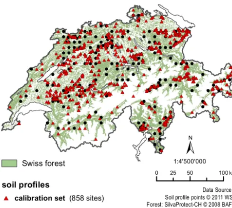
As our study focused on forest soils, we had to delimit the forest area of Switzerland (Fig. 2). We used the same criteria as Giamboni (2008): six categories rendered by VECTOR25 (Swisstopo, 2011b) as forest plus former forest areas, dev-astated in 1990 and 1999 by two hurricanes (Bundesamt für Umwelt BAFU, 2010) and currently not classified as forest by VECTOR25. Areas shared with the National Mire Inven-tory (FOEN, 2012b) were excluded. This removed some but not all organic soils because the inventory does not cover all bogs and fens under forest, in particular, if these had been drained in the past.

According to this definition, forests cover 11 800 km2 (29 % of total area of Switzerland). Forests extend over altitudes from 190 to 2390 m above sea level (Swisstopo, 2011a). Climatic conditions therefore vary notably within this area: mean annual precipitation ranges from 600 to 2900 mm and mean annual temperature from −1 to 13◦C (MeteoSwiss, 2011). Two thirds of the forested area is dom-inated by coniferous trees, deciduous forests prevail only at lower altitudes in the regions Jura, Central Plateau, Pre-Alps and Southern Alps (Swiss Federal Statistical Office, 2000b). Considerable variation is also found in geologic parent ma-terial for soil formation: predominantly limestones in Jura and in parts of the Pre-Alps, fluvioglacial sediments of sev-eral Quaternary glaciations and of the Tertiary on the Central Plateau, and igneous and metamorphic rocks in the Alps and Southern Alps. This large variation of pedogenetic factors is reflected in the development of very diverse soils (Walthert et al., 2004) with variable conditions for mineralisation and accumulation of SOC.

2.2 Data 2.2.1 Soil data Soil profiles

(4)

! ! ! ! ! ! ! ! ! ! ! ! ! ! ! ! ! ! ! ! ! ! ! ! ! ! ! ! ! ! ! ! ! ! ! ! ! ! ! ! ! ! ! ! ! ! ! ! ! ! ! ! ! ! ! ! ! ! ! ! ! ! ! ! ! ! ! ! ! ! ! ! ! ! ! ! ! ! ! ! ! ! ! ! ! ! ! ! ! ! ! ! ! ! ! ! ! ! ! ! ! ! ! ! ! ! ! ! ! ! ! ! ! ! ! ! ! ! ! ! ! ! ! ! ! ! ! ! ! ! ! ! ! ! !!!!! ! !!!! ! ! !!!!! ! ! !! ! !!!_! !_!!!!! !!!!! ! # * # * # * # * # * # * # * # * # * # * # * # * # * # * # * # * # * # * # * # * #* # * # * # * # * # * # * # * # * # * #* # * # * # * # * # * # * # *#* # * # * # * # *#* # * # * # * # * # * # * # * # * # * # * # * _#_* # * # * # * # * # * # * # * # * # * # * # * # * # * # * #* # * # * # * # * # *#* # * _*_#_*_##*#*#*#**##*#*#* # * # * # *#* # * # * _#_*_#_* # * # * # * #*#* # **# _#_*_#_*_*_#_#_*_#_*_#_*#* # *#* # * # * # * # * # * # * # * # *#*#*#* # * # * # * # *#*#* # * # * # * # * # * # * # * # *#*#* # * # * # * # * # * # * # * # * # *#*#*#*#* # *#* # * # *#*#*#*#*#*#* # * # * # *#* # * # * # * # * # * # * # * # * # * # * # * # * # * # * # * # * # *#*#*#*#*#*#* # * #* # * # * # * # * # * # *#*#* # *#* # * # *#* # * # * # * # * # * # *#*_#_* # * # * # * # * # * # *#*#* # * # *#* # * # * # * # * # * # * # * # * # * # * # *#* #*#* # * # * # *#**#*###*#*#*#**#* # * # * # * # * # * # *#* # * # * # * # * # * # * # * # *#* # *#*#* # * # *#* # * # *#* # * # * # * # * # * # * # * # * # * # * # *#*#* # * # * # * # * # * # *#* # * # * # * # * # * # *#*#* # * # * # * # * # * # * # * # *#*#*#* # * # * # * # * # * # * # *#*_#_* # * # * # * # *#* # *#*#* # * # * # * # * # * # *_#_* # *#*#*#* # * # * # * # * # * # * _#_*#* # * # * # * # * # *#* # * # * # * # * # * # * # * # * # * #* # * # * # * # * # * # * # * # * # * # *#* #*#*#* # * # * # * # * # *_#_* # * # * # * # *#* # *#* # * # *#* # * # *#*_#_* # * # * # * # * # * # * # * # * _#_* # *#*#*#*#*#* # * # * # * # * # * # **##*#* #*#*#*#*#**#*##* # * # * # * # * # * # * # * # * # * # *#* # * # * # * # * # * # * # * # * # * # * # * # * # *#* # * # * # * # * # * # * # * # * # * # * # * # * # * # * # * # * # * # * # * # * # *#*#*#* # * # * # * # * # * # * # * # * # * # * # * # * # *_#_*_#_*_#_* # * # *#*#* # *#* # * # * # * # **#*#*##**##* #*#*#*#* # * # *###**#***###*#***##*#*#* # * # * # * # * # *#* # *_#_* # * # * # * # * # * # * # * # **##*#*#*#***##*##*_#_*_#*_*##*##**#*#* # * # * # * # * # * # * # * # * # * # * # * # * # * # * # * # * # * # * # * # * # * # * # * # * # * # * # * # * # * # * # * # *#* # * # * # * # * # * # * # * # * # * # * # * # * # * # * # * # * # * # * # * # *#* # * # * # * # * # * # * # * # * # * # * # * # * # * #*#*_#_*_#_*_#_* # * # * # * # * # * # *#*#*_#_*#*_#_*_#_* # *#* # * # * # * # * # * # * # * # *#*#*#*#*#*#* # *#*#*#*#*#*#* # *#*#* # *#*#*#*#**#**##*##*#*#*#* # * # *#* # * # *#*#*#**##*#*#*#* # *#* # * # * # * # * # * # * # * # * #*#* # * # * # * # * # * # * # * #* # * # * # * # * # * # * # * # * # * # * # * # *#* # * # * # * # *#* # * # * # * # * # * _#_* # *#*#*#* # * # *#* # * # * # * # * # * # * # * # * # *#*#* # *#* # * # * # * # * # * # * # * # *#* # * # *#* #* # * # * # *#*#*#*#*#*#* # * # * # *_#_*_#_* # *#* # * #*#*#*#*#* # * # * # * # * # * # * # * # * # * # * # * # * # *#*#*#* # *#*#*_#_*#*#* # *#* # * # * # * # **##*#*#*#*#**#*#*# # * # * # * # * # *#* # * # * # * # * # * # * # * # *#* # * # *#*#*#*#*#* # *_#_*#*#*

0 25 50 100km

±

calibration set (858 sites)

soil profiles

validation set (175 sites)

Swiss forest 1:4'500'000

! # *

Figure 2. Locations of the 1033 soil profiles and Swiss forest area (subdivided into calibration and validation sets).

profiles was recorded in the field on topographic maps (scale 1:25 000), hence the error in the coordinates is about±25 m. We assigned 175 out of the 1033 soil profiles to the valida-tion set, which was used to check the predictive power of the fitted statistical models, and the remaining 858 soil profiles were used as a calibration set, used to build and fit these mod-els. All except three sites of the validation set with organic soils lay on the 1 km (38 sites) and 8 km grid (134 sites). This selection resulted in a fairly even and spatially repre-sentative distribution of the validation sites across Switzer-land (Fig. 2). When splitting the data, we strived for a bal-anced representation of soil map units and vegetation types between calibration and validation set.

The thickness of all soil horizons was recorded in the field on the faces of soil pits and subsequent soil sampling and laboratory analyses were all done by pedogenetic horizons. Stone content

The volumetric content of stones (particles with size > 2 mm) was estimated visually on the face of soil profiles, which is a common procedure (Baritz et al., 2010). These estimates are bound to some error that is very difficult to quantify because surveys were done by different staff. How-ever, neglecting stone content as in many other studies (e.g. Krogh et al., 2003; Meersmans et al., 2008; Xu et al., 2011) would lead to overestimation of SOC stocks as stone content is large for many Swiss forest soils.

Soil density

The density of the soil fraction with particle size≤2 mm was measured for 440 out of about 5000 mineral soil horizons

with soil samples of fixed volume (Walthert et al., 2004, p. 702) collected from the soil profiles. In addition, a field estimate (penetration resistance of blade) of soil density was available for all soil horizons (ordinal variable with 5 cate-gories, Walthert et al., 2004, p. 695).

We computed the median of the measured densities for each category of this variable and assigned these medi-ans to all soil horizons without density measurements. The accuracy of this pedotransfer function (PTF) was evalu-ated by tenfold cross-validation (by estimating and re-assigning the median densities computed from nine cross-validation subsets to the 10th subset). The median of the cross-validation errors was equal to 0.002 g cm−3 and the median absolute deviation (MAD, see below) was equal to 0.256 g cm−3. For comparison, we used also the PTF by Adams (1973) and Honeysett and Ratkowsky (1989), which performed best for forest soils in the evaluations of De Vos et al. (2005) and Baritz et al. (2010). Bias and MAD of the cross-validation errors ranged between 0.33–0.34 and 0.50– 0.52 g cm−3 without re-calibration and if the coefficients of the PTF were re-estimated with our own data these measures were 0.06 and 0.30 g cm−3. Hence, our PTF had better pre-dictive power than the PTF by Adams, but it was worse than the one by Jalabert et al. (2010) who recalibrated their PTF by ML methods.

SOC content

SOC content was measured for all mineral soil samples by an elemental C/N analyser (combustion at 1000◦C, Walthert et al., 2010). When pH of a soil sample was larger than 6.0 then carbonates were removed by fumigation with hy-drochloric acid prior to measuring C. Below this pH car-bonates were assumed to be absent, and the OC content of the sample was assumed to be equal to its total C content (Walthert et al., 2010).

SOC stock

The SOC stockSi stored in horizoniper unit area [kg m−2] was calculated from the thickness Di of the horizon [m], its volumetric stone content Gi [m3m−3], soil density ρi [kg m−3] and its SOC contentCi[kg kg−1] by

Si=Di(1−Gi)ρiCi, (1)

and the stockS in a given depth compartment was summed by

S= h

X

i=1

wiSi, (2)

(5)

2.2.2 Covariates for statistical modelling Parent material and soil

Detailed information on soils and parent material is not avail-able for the whole of Switzerland. Therefore, an overview soil map discriminating 25 units (map scale 1:200 000, Swiss Federal Statistical Office, 2000a) was used as a coarse representation of geologic and pedogenetic conditions. Be-ing mainly designed for agricultural usage, certain map units did not well reflect contrasting conditions of forest soil devel-opment. To lessen this drawbacks five additional units were created by intersecting the soil map with selected polygons of the Geological Map of Switzerland (map scale 1:500 000, Swisstopo, 2005) and the maps of the Last Glacial Maximum (map scale 1:500 000, Swisstopo, 2009) and of the biogeo-graphic regions of Switzerland (see Table S2 in Supplement, Gonseth et al., 2001). Besides, we used the geotechnical map (map scale 1:200 000, BFS, 2001) to extrapolate soil infor-mation available only at the 1033 soil profile sites (for de-tails on sampling see Appendix 2, Walthert et al., 2004) to the whole of Switzerland. Median values of soil properties measured at those sites that lay within a given geotechni-cal map unit were assigned to the respective unit. Then we checked whether these newly generated covariates correlated with SOC stocks. This was true for cation exchange capacity, iron and calcium stocks and mass of soil particles <2 mm that we consequently retained for the statistical analyses. Climate

Three climate data sets were available to us with spatial in-formation on mean annual/monthly temperature and precipi-tation, cloud cover, sunshine duration, radiation, degree days, continentality index (Gams, 1935), temperature variation, ra-tio of actual to potential evapotranspirara-tion and site water balance (Grier and Running, 1977). Two data sets contained spatial information (resolution 25 m and 2 km, respectively) on climatic means for period 1961–1990 (Zimmermann and Kienast, 1999; MeteoSwiss, 2011) and the third for 1975– 2010 (spatial resolution 250 m). Since it was not a priori clear which data set would be best, we used them all as covariates in the statistical analyses.

Vegetation

The percentage of coniferous trees was derived from spec-tral imagery (Swiss Federal Statistical Office, 2000a) and species composition data of the National Forest Inventory (NFI, Brassel and Lischke, 2001, both covariates rasterised with 25 m resolution). The SPOT5 mosaic of Switzerland (Mathys and Kellenberger, 2009) with spectral reflectance in green, red and near-infrared bands, band ratios, IHS colour space transformations and the normalised difference vege-tation index (NDVI, Kriegler et al., 1969) were available. Moreover, canopy height (difference of digital surface to

digital elevation model of 2 m resolution, Swisstopo, 2011a) was included in the set of covariates.

Topography

Two digital elevation models (DEM, resolution 2 and 25 m, Swisstopo, 2011a) allowed to compute a broad range of ter-rain attributes covering multiple scales: elevation, slope an-gle, aspect, north and east directions, planar, profile and com-bined curvatures and smoothed versions of these attributes. Furthermore, topographic position indices were calculated based on Zimmermann (2000) and Jenness (2006) with radii ranging from 6 m to 2 km. Flow accumulation area and topo-graphic wetness indices were computed by single and multi-flow algorithms (Tarboton, 1997).

Accounting for errors in locations of soil profiles

We mentioned above that coordinates of soil profiles had been recorded with a likely error of about ±25 m, which clearly exceeds the resolution of the highly resolved DEM. Therefore, the values of all covariates were averaged for cir-cular neighbourhoods, centred on the recorded profile loca-tions and having radii equal to 13, 19 or 26 m. Depending on the type of data, different summary statistics were computed: arithmetic means for real numbers, medians for integers and the most frequent category for nominal or ordinal variables. However, values of covariates aggregated with the different radii were highly correlated, Therefore, for statistical analy-ses we only used summaries computed with a radius of 26 m. 2.3 Statistical analyses

2.3.1 Model

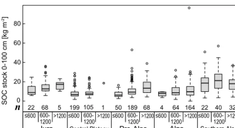
Given past experiences (Mishra et al., 2010; Kumar et al., 2012; Wiesmeier et al., 2012) and exploratory analyses (Fig. 3), we decided to use a log-normal model for the SOC stockS(s)at locations:

Y (s)=log(S(s))=x(s)Tβ+Z(s)+ε(s), (3) wherex(s)Tβ is the external drift that accounts for depen-dence ofS on environmental covariatesx, (withβ the re-gression coefficients), T denotes transpose andZ(s)is a sta-tionary autocorrelated Gaussian random field with zero mean and isotropic exponential variogram with sillσ2and rangeα

γ (h)=σ2(1−exp(−h/α)) . (4)

(6)

Figure 3. Boxplots of calculated soil organic carbon (SOC) stocks in 0–100 cm depth by ecoregion and altitudinal class (n: number of sites).

2.3.2 Model building

We used only the calibration set for model building, which involved the following steps:

1. Positively skewed covariates (e.g. some terrain at-tributes) were transformed by square root or natural log-arithm.

2. Strongly correlated and therefore redundant covariates were eliminated based on correlation biplots (Gabriel, 1981).

3. The least absolute shrinkage and selection operator (LASSO, Hastie et al., 2009, Sect. 3.4) – an algorithm that likely excludes non-relevant covariates – was used with various sets of covariates, partly enriched by first-order interactions between pairs of covariates, to find an external drift that minimised the mean squared error (MSE) in tenfold cross-validation.

4. The parameters of the geostatistical model (Eq. 3) were then estimated by a novel robust restricted maximum method (REML, Künsch et al., 2011, 2014) for the ex-ternal drift selected by LASSO.

5. Still using the external drift of the optimal LASSO fit, an optimal value of the tuning constantcthat controls the robustness of REML was chosen by tenfold cross-validation. We used the continuous ranked probability score (CRPS, see below and Gneiting et al., 2007) as main criterion for choosing the tuning constant (and for selecting covariates in step 6). We further tested whether other variogram functions (spherical, Whittle–Matérn, etc., e.g. Diggle and Ribeiro Jr., 2007) improved the fit but this was not the case.

6. Non-relevant covariates were then removed step by step by tenfold cross-validating the robust REML fit (and added back along with interaction terms at later stages if cross-validation results justified this).

7. The levels of categorical covariates (in particular of the soil map) were merged based on partial residual plots (e.g. Faraway, 2005) and cross-validation CRPS to ob-tain a final parsimonious geostatistical model.

The improvement of the cross-validation MSE from step 3 to 7 is shown in Fig. S1 of the Supplement.

2.3.3 Evaluating predictive performance of statistical models

The predictive power of the fitted geostatistical models was tested by comparing predicted (Eq. 15) with calculated SOC stocks (Eq. 2). The same criteria were used in model build-ing by cross-validation (see above). Marginal bias and overall precision were assessed by

BIAS= −1 n

n

X

i=1

(S(si)− ˜S(si))

S(s_i) , (5)

robBIAS= −median1≤i≤n

S(si)− ˜S(si) S(s_i)

!

, (6)

RMSE=





1 n

n

X

i=1

S(si)− ˜S(si) S(si)

!2

 1/2

, (7)

robRMSE=MAD1≤i≤n

S(si)− ˜S(si) S(si)

!

, (8)

whereS(s_i)stands for calculated,S(˜ s_i)for predicted SOC stocks and MAD for median absolute deviation. We com-puted summaries of the relative prediction errors because the log-normal model implies constant relative dispersion (i.e. constant coefficient of variation). We standardised the pre-diction errors bySinstead ofS˜to have a common standardi-sation when comparing different models.

We also computed a standard and robustR2by R2= Cov[S(si),

˜ S(si)]2

Var[S(si)]Var[ ˜S(si)]

, (9)

robR2=

1−

Pn

i=1|S(si)− ˜S(si)|

Pn

i=1|S(si)−median1≤i≤n(S(si))|

!2

. (10) Although the latter is tailored for robust L1 regression (Croux and Dehon, 2003), we found it useful for our approach.

In addition, we computed the strictly proper scoring cri-terion CRPS (Gneiting et al., 2007), which is equal to the integral over the Brier score (BS):

CRPS=

∞

Z

−∞

BS(u)du

≈ n

X

i=1

(7)

where S(i) is the ith largest calculated stock, S(0)=S(1), S(n+1)=S(n)and

BS(u)= 1 n

n

X

i=1

{ ˜Fi(u)−I (S(si)≤u)}2, (12)

where_F˜

i(u) is the (estimated) log-normal predictive distri-bution function of the ith datum and I (A) is an indicator equal to one if A is true and zero otherwise. CRPS mea-sures the sharpness of predictive distributions (smaller val-ues signal sharperF˜i), hence depends both on prediction pre-cision and quality how prediction uncertainty is modelled. Modelling of prediction uncertainty was further tested by counting how many observations fall into two-sided 95 %-prediction intervals and by checking the empirical distribu-tion of the probability integral transform (PIT, Gneiting et al., 2007)

PITi= ˜Fi(S(si)), (13)

which should be uniformly distributed.

2.3.4 Mapping SOC forest soil stocks across Switzerland

To get better parameter estimates for finally mapping SOC stocks by EDK we fitted the model to the merged calibration and validation data. This was done after computing valida-tion statistics (see above). SOC stocks were then predicted by robust log-normal kriging (Cressie, 2006; Künsch et al., 2014) for the nodes of a 100 m grid by

˜

S(s)=exp(Y (˜ s)+1/2{ ˆτ2+ ˆσ2−Var[ ˜Y (s)]}), (14) with

˜

Y (s)=x(s)Tβˆ_θˆ+γ_θˆ(s)T0 −1

ˆ

θ ˆ

Z_θˆ, (15)

whereˆdenotes robust REML estimates,γ_θˆ(s)is the vector

with the estimated covariances between Z andZ(s),0_θˆ is

the estimated covariance matrix of Z and Var[ ˜Y (s)] =γ_θˆ(s)T0−_ˆ1

θ ,x(s)

T ₍₁₆₎

·Cov

"

ˆ Z_θˆ

ˆ

β_θˆ

!

,

ˆ ZT_ˆ

θ, ˆ

βT_ˆ

θ

#

0−_ˆ1

θ γθˆ(s)

x(s)

!

.

Künsch et al. (2011) give in their Eq. (19) an approxima-tion for the covariance matrix of(ZˆT_ˆ

θ, ˆ

βT_ˆ

θ). Approximate, log-normal kriging variances were obtained from

Var[S(s)− ˜S(s)] =exp2x(s)Tβˆ_θˆ+ ˆτ2+ ˆσ2

(17) · {exp(τˆ2+ ˆσ2)−2 exp(Cov[ ˜Y (s), Y (s)])

+exp(Var[ ˜Y (s)])},

where

Cov[ ˜Y (s), Y (s)] =bγ_θˆ(s)T0−_ˆ1

θ ,x(s)

T ₍₁₈₎

·M−1

γ_θˆ(s)

XTγ_θˆ(s)

andb, X, M as in Künsch et al. (2011). Since outliers re-ceive small weight when computingβˆ_θˆandZˆ_θˆby the robust

REML algorithm, the prediction of SOC stock by Eqs. (14) and (15) is also insensitive to outlying observations.

2.3.5 Predicting regional and national mean SOC stocks The mean SOC stocks in the five ecoregions (and for the whole of Switzerland), stratified by altitude, were computed from the robust log-normal point kriging predictions at the nodes of the 100 m grid by

˜

S(Bk)=1/Nk X

si∈Bk

˜

S(si), (19)

where the notationP

si∈Bk means summation over theNk

nodes of the grid falling into region Bk. Equation (19) is

a discrete approximation to the log-normal block kriging pre-dictor (e.g. Cressie, 2006, Eq. 14). The block kriging vari-ance (i.e. the varivari-ance of the prediction error,S(Bk)− ˜S(Bk))

for regionBkcan similarly be approximated by the

covari-ance (Eq. S2 in Supplement)

Var[S(Bk)− ˜S(Bk)] =

1 N_k2

X

si∈Bk X

sj∈Bk

Cov[S(s_i)− ˜S(s_i), S(s_j)− ˜S(s_j)]. (20)

However,Nk is usually too large (in our case: 104–105) to

evaluate the double sum of Eq. (20) in acceptable comput-ing time. We used therefore a Monte Carlo approximation for Eq. (20), where the covariances were repeatedly com-puted and averaged for randomly selected subsets of nodes inBk. Full details can be found in the respective appendix of

the Supplement. Of course, this approximation can also be used if there is no residual autocorrelation, and it is straight-forward to derive analogous expression for untransformed data. For sufficiently large regions, one can safely assume – due to the central limit theorem – that the prediction errors S(Bk)− ˜S(Bk)are normally distributed, in spite of the fact

that point prediction errors follow log-normal laws.

(8)

3 Results

3.1 Calculated SOC stocks

SOC stock stored in the top 30 cm of the mineral soil at the 1033 sites varied considerably from 0.8 to 36.1 kg m−2 (me-dian 6.3 kg m−2), and to 100 cm depth stocks ranged from 1.0 to 96.4 kg m−2 (median 9.2 kg m−2). Stocks in both depths were strongly correlated (Spearman correlation 0.91). On av-erage, calculated stocks were slightly larger for the validation set (Table S1 of Supplement). Except for the Central Plateau and the Southern Alps, mean stocks down to 1 m depth in-creased with altitude (Fig. 3). For most strata, the frequency distribution of stocks was positively skewed and dispersion increased with the mean, calling for log-transformation for the statistical analyses.

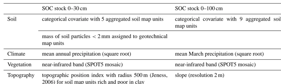
3.2 Models for SOC stocks in 0–30 and 0–100 cm depth Not surprisingly, given the strong correlation of stocks in the two depths, the structure of the external drifts did not differ much. Both drifts were parsimonious, with 10 and 12 fitted coefficients, respectively, and included covariates character-ising soils, vegetation, climate and topography (see Table 1 as well as Tables S3 and S4 of Supplement).

Tenfold cross-validation resulted for both depths in simi-lar robR2(0.31). However, based on CRPS, the fit was better for topsoil stocks (0.238 vs. 0.252). Residuals of both mod-els were spatially autocorrelated, but spatial dependence was rather weak with nugget/total-sill ratios and effective ranges of 0.37 and 600 m for 0–30 cm and 0.41 and 660 m for 0– 100 cm depth (see Table S5 of Supplement).

The optimal tuning constant was equal toc=2 for both models, and robustly estimated parameters fitted the data slightly better than customary Gaussian REML estimates (cross-validation CRPS of 0.239 for non-robust model fit for 0–30 cm and of 0.253 for 0–100 cm depth).

3.3 Validation of SOC stock predictions with independent data

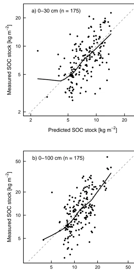
Figure 4 shows calculated SOC stocks in 0–30 and 0–100 cm of the mineral soil, plotted against respective predictions for the independent validation set. The solid lines of the loess scatterplot smoothers (Cleveland, 1979) are close to the 1:1 lines, indicating absence of conditional bias. This is con-firmed by the BIAS and robBIAS statistics (Table 2). Irre-spective how the statistics were computed, relative marginal bias was less than 15 %. However, variation of the data around the 1:1 line was quite large, which was reflected in large root mean squared relative errors. robRMSEs were about 40 % and non-robust RMSE 49 % for topsoils and 56 % for stocks down to 100 cm. As seen from the robust R2, the models explained about 34 % of the variation of calcu-lated SOC stock in 0–30 cm and 40 % of calcucalcu-lated SOC stock in 0–100 cm. The kriging variances overestimated the

● ● ● ● ● ● ● ● ● ● ● ● ● ● ● ● ● ● ● ● ● ● ● ● ● ● ● ● ● ● ● ● ● ● ● ● ● ● ● ● ● ● ● ● ● ● ● ● ● ● ● ● ● ● ● ● ● ● ● ● ● ● ● ● ● ● ● ● ● ● ● ● ● ● ● ● ● ● ● ● ● ● ● ● ● ● ● ● ● ● ● ● ● ● ● ● ● ● ● ● ● ● ● ● ● ● ● ● ● ● ● ● ● ● ● ● ● ● ● ● ● ● ● ● ● ● ● ● ● ● ● ● ● ● ● ● ● ● ● ● ● ● ● ● ● ● ● ● ● ● ● ● ● ● ● ● ● ● ● ● ● ● ● ● ● ● ● ● ● ● ● ● ● ● ●

Predicted SOC stock [kg m−2]

Measured SOC stock [kg

m

−

2 ]

2 5 10 20

a) 0−30 cm (n = 175)

● ● ● ● ● ● ● ● ● ● ● ● ● ● ● ● ● ● ● ● ● ● ● ● ● ● ● ● ● ● ● ● ● ● ● ● ● ● ● ● ● ● ● ● ● ● ● ● ● ● ● ● ● ● ● ● ● ● ● ● ● ● ● ● ● ● ● ● ● ● ● ● ● ● ● ● ● ● ● ● ● ● ● ● ● ● ● ● ● ● ● ● ● ● ● ● ● ● ● ● ● ● ● ● ● ● ● ● ● ● ● ● ● ● ● ● ● ● ● ● ● ● ● ● ● ● ● ● ● ● ● ● ● ● ● ● ● ● ● ● ● ● ● ● ● ● ● ● ● ● ● ● ● ● ● ● ● ● ● ● ● ● ● ● ● ● ● ● ● ● ● ● ● ● ●

Predicted SOC stock [kg m−2]

Measured SOC stock [kg

m

−

2 ]

5 10 20 50

5 10 20

50 b) 0−100 cm (n = 175)

Figure 4. Scatter plots of measured against predicted soil organic carbon (SOC) stocks in 0–30 cm (a) and 0–100 cm (b) of the min-eral soil, computed with the calibration data for the sites of the val-idation set (solid line: loess scatter plot smoothers,n: number of sites).

(9)

Table 1. Covariates of external drift selected by model building procedure for soil organic carbon (SOC) stocks in 0–30 cm and 0–100 cm depth.

SOC stock 0–30 cm SOC stock 0–100 cm

Soil categorical covariate with 5 aggregated soil map units categorical covariate with 9 aggregated soil map units

mass of soil particles<2 mm assigned to geotechnical map units

Climate mean annual precipitation (square root) mean March precipitation (square root)

Vegetation near-infrared band (SPOT5 mosaic) near-infrared band (SPOT5 mosaic)

Topography topographic position index with radius 500 m (Jeness, 2006) for soil map units rich and poor in clay

slope (resolution 2 m)

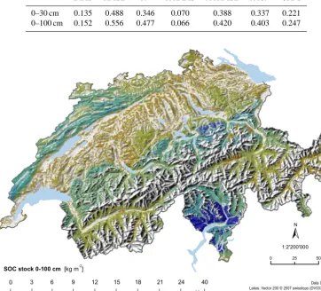
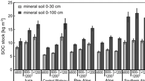
3.4 Prediction of SOC stocks for Swiss forest soils For computing the predictions, the parameters of the final models (Table 1) were estimated with data of 1022 sites (combined calibration and validation sets, excluding 11 sites with missing covariate information). Robust log-normal krig-ing predictions of stocks stored to 100 cm depth are mapped in Fig. 5 for the nodes of the 100 m grid. The map with the predicted topsoil SOC was very similar and is therefore not shown. Block kriging predictions of the mean stocks for the five ecoregions and for the entire Swiss forest area are shown in Fig. 6.

The largest SOC stocks were predicted for higher altitudes and for the Southern Alps in general. Predicted stocks were smallest for the Central Plateau and for lower altitudes of the Pre-Alps, where stocks down to a depth of 100 cm remained below 10 kg m−2_{. For the whole of Switzerland, predicted}

mean SOC stocks in 0–30 cm were equal to 7.99 kg m−2_(SE

0.15 kg m−2, 95 %-prediction interval [7.69, 8.29] kg m−2). Down to 100 cm a SOC stock of 12.58 kg m−2SOC was pre-dicted (SE 0.24 kg m−2) resulting in a 95 %-prediction inter-val of [12.11, 13.05] kg m−2. Thus, about 4.5 kg m−2 SOC are stored in subsoils (30–100 cm) of Swiss forests.

Our estimates do not include carbon stored in forest floor horizons. Spatially explicit estimation was not possible for this compartment because we largely lacked C and soil density measurements. Based on the available data, Nuss-baum et al. (2012) estimated that about 1.7 kg m−2 (SE 0.08 kg m−2) of C are stored in forest floors of Swiss forests.

4 Discussion

4.1 Model building and covariate selection

The model building procedure effectively reduced the 360 potential covariates and their first-order interactions to a small and meaningful set. Precipitation was a covariate of both models (with positive coefficients, Figs. S2 and S3 in

Supplement). Perruchoud et al. (2000), Martin et al. (2011), Meersmans et al. (2012b), Kumar et al. (2012), Chiti et al. (2012) and Wiesmeier et al. (2013) previously reported that wet climate favours SOC accumulation. Near-infrared re-flectance of the forest canopy was also selected for both mod-els: smaller reflectance of conifers for wavelength of 750 to 1300 nm (Cipar et al., 2004) and negative regression co-efficients imply larger SOC stocks under conifers than de-ciduous trees. Additionally, information on parent material was important for SOC prediction: aggregated units of the overview soil map were meaningful covariates despite repre-senting the heterogeneous pedogenetic conditions typical for Switzerland only coarsely (see Figs. S2 and S3 in Supple-ment).

4.2 Residual spatial autocorrelation

Spatial autocorrelation of residuals remained weak in both models, suggesting that spatial patterns in calculated SOC stocks were reasonably well modelled by the external drifts. Due to short-ranged spatial dependence, only 5 % of the nodes of the prediction grid were within a distance equal to the effective variogram ranges of the soil profile sites. From the validation set only 14 of 175 sites were within these zones. Neglecting spatial autocorrelation but using the same set of covariates would slightly lower the precision of SOC stock estimates for the 0–30 cm and increase precision for the 0–100 cm depth compartment (Table S6 in Supplement). Although kriging predictions differ only within the estimated range of spatial dependence from predictions obtained by the regression models, consideration of autocorrelation was im-portant for accurate modelling of prediction uncertainty. 4.3 Robust parameter estimation

(10)

Table 2. Statistics of relative prediction errors of soil organic carbon (SOC) stocks in two depth compartments (0–30, 0–100 cm) for the validation set.

BIAS RMSE R2 robBIAS robRMSE robR2 CRPS

0–30 cm 0.135 0.488 0.346 0.070 0.388 0.337 0.221 0–100 cm 0.152 0.556 0.477 0.066 0.420 0.403 0.247

0 25 50km

±

1:2'200'000 SOC stock 0-100 cm [kg m-2_]

0 3 6 9 12 15 18 21 24 40

Figure 5. Robust log-normal kriging prediction of the soil organic carbon (SOC) stock in 0–100 cm of the mineral soil of Swiss forests (computed with best-fit model with covariates according to Table 1 and tuning constantc=2, smoothed with focal mean with a radius of 1 pixel=100 m).

increase of robRMSE (0.6 % for SOC stock predictions in 0–30 cm and 0.5 % for stocks in 0–100 cm) compared to a non-robust fit of the model with the same covariates (Ta-ble S6 in Supplement). A further advantage of robust esti-mation is clear labelling of data that are fitted only poorly by the models. Scrutinising environmental conditions for those observations revealed that these were: (i) sites on calcare-ous bedrock in inner Alpine valleys where recurring drought hinders OC mineralisation, resulting in thick forest floor and SOC rich A horizons (Walthert et al., 2004); and (ii) sites in the Southern Alps with acid podsolic soils that show pro-nounced humus translocation down the profile. Moreover, these sites are influenced by forest fires (leading to accu-mulation of black carbon) and stabilise SOC effectively by large content of aluminium and iron weathered from silicate rich bedrock (Blaser et al., 1997). Using robust procedures ensured that SOC data resulting from sites subject to such special conditions did not confound statistical analyses.

4.4 Predictive performance of fitted models

(11)

Figure 6. Block kriging predictions of the soil organic carbon (SOC) stocks in 0–30 cm and 0–100 cm soil depth in the five ecore-gions stratified by altitude a.s.l. (m) into three classes (vertical lines: prediction intervals).

On the one hand, incompleteness and partly insufficient quality of covariates is likely responsible for the modest pre-dictive power of the fitted models. In particular, spatial in-formation on soil or vegetation parameters controlling SOC turnover was completely lacking in our set of potential co-variates. Also, data on forest management and land use his-tory (e.g. stand age), found to be relevant by Schroeder et al. (2009) and Schulp et al. (2013), was missing.

On the other hand, causes for the moderate precision of our predictions lie in the missing soil density measurements (Schrumpf et al., 2011). For most horizons soil density was derived from a PTF, which proved to be unbiased, but never-theless added additional variation to the data.

4.5 Spatial structure of SOC stock predictions

So far, no maps of SOC stocks have been published for Swiss forests that could be used for verification of Fig. 5. Never-theless, several patterns in our SOC stock map matched our expectations: small SOC stock was predicted for acid soils at lower altitude on the Central Plateau. Very small total SOC stock was estimated for areas in the eastern Pre-Alps and Alps where Permian Verrucano sand stones form the bedrock. On these sites, SOC accumulates in the forest floor. The map shows large stocks up to 40 kg m−2in parts of the eastern Pre-Alps where large annual precipitation and water-logged soils prevail, and also in the Jura region, where large stocks are likely related to organic matter stabilisation by cal-cium (Walthert et al., 2004). Very large SOC stock was pre-dicted for the Southern Alps, where a combination of forest fires and Al-rich soil on metamorphic parent material led to an accumulation of organic matter, even in deeper soil hori-zons. Excepting the special conditions in the Southern Alps, predictions of the mean stocks by ecoregions and altitudinal class (Fig. 6) reflected the increase of SOC stock with alti-tude described by Hagedorn et al. (2010).

4.6 Comparison with SOC stock estimates of previous studies

Perruchoud et al. (2000) estimated for the whole of Switzer-land a mean SOC stock of 7.59 kg m−2 (SE 0.30 kg m−2) for the top 30 cm of the mineral soil and 9.82 kg m−2 (SE 0.53 kg m−2) for mineral soils down to bedrock, which are both significantly smaller than our current estimates (p val-ues of one-sidedz tests: 0.004 and<10−12, respectively). The estimate of 11.86 kg m−2(SE 0.54 kg m−2) by Bolliger et al. (2008) for total SOC stock (forest floor plus mineral soil down to bedrock) of Swiss forests is also smaller than our estimate for 0–100 cm. Our standard errors (0–30 cm: 0.15 kg m−2_{; 0–100 cm: 0.24 kg m}−2_{) are smaller (by a}

fac-tor of about two) than those of Perruchoud et al. (2000) and Bolliger et al. (2008). Since we validated uncertainty mod-elling for point predictions and used a coherent framework to quantify the uncertainty of our regional and national mean estimates, one can trust that these figures accurately represent the uncertainty of our estimates.

Perruchoud et al. (2000) estimated that about 77 % of SOC stock of Swiss forests is stored in the mineral topsoil (0– 30 cm), whereas we predicted a proportion of only 64 %, which matches the proportion of 64.3 %, computed directly from the observed SOC data (n=1033) very well.

5 Summary and conclusion

Greenhouse gas reporting requires estimates of regional or national mean SOC stocks that are computed from observa-tions with quasi point support. The geostatistical block krig-ing approach is the method of choice for such change-of-support problems as it guarantees that estimates are unbi-ased and precise and prediction standard errors correctly ac-count for the spatial averaging. Rather surprisingly, our study seems to be the first to employ such an approach in the con-text of GHG reporting.

Based on spatially referenced data about 1033 soil profiles, we built parsimonious, pedologically interpretable, geosta-tistical models for SOC stocks in two depth compartments (0–30, 0–100 cm) of mineral soils of Swiss forests. The mod-els relate calculated stocks to environmental covariates that characterise the pedogenetic conditions at the profile sites and account for residual spatial auto-correlation. The fitted models were rigorously validated by comparing predictions with independent data. Using the models, we mapped forest SOC stock across Switzerland by robust external-drift krig-ing at high spatial resolution and aggregated the krigkrig-ing re-sults coherently to come-up with reliable block kriging esti-mates (and standard errors) of national mean SOC stocks in Swiss forests.

(12)

our (independently validated) standard errors were only half as large as the previously reported SE. As we used a sub-stantially larger database and sound geostatistical methods, we trust our estimate more and conclude that SOC stocks of Swiss forests have been considerably underestimated in the past.

The Supplement related to this article is available online at doi:10.5194/gmd-7-1197-2014-supplement.

Acknowledgements. We thank the Swiss Federal Office for the

Environment (FOEN) for funding this work. A special thank goes to the WSL for collecting and analysing innumerable soil samples and to the WSL GIS group for providing the infrastructure for spatial data processing.

Edited by: M.-H. Lo

References

Adams, W. A.: The effect of organic matter on bulk and true densi-ties of some uncultivated podzolic soils, J. Soil Sci., 24, 10–17, doi:10.1111/j.1365-2389.1973.tb00737.x, 1973.

Arrouays, D., Deslais, W., and Badeau, V.: The carbon content of topsoil and its geographical distribution in France, Soil Use Man-age., 17, 7–11, 2001.

Baritz, R., Seufert, G., Montanarella, L., and Ranst, E. V.: Carbon concentrations and stocks in forest soils of Europe, Forest Ecol. Manag., 260, 262–277, doi:10.1016/j.foreco.2010.03.025, 2010. BFS: GEOSTAT Benützerhandbuch, Bundesamt für Statistik, Bern,

2001.

Blaser, P., Kernebeek, P., Tebbens, L., van Breemen, N., and Lus-ter, J.: Cryptopodzolic soils in Switzerland, Eur. J. Soil Sci., 48, 411–423, doi:10.1111/j.1365-2389.1997.tb00207.x, 1997. Bolliger, J., Hagedorn, F., Leifeld, J., Böhl, J., Zimmermann, S.,

Soliva, R., and Kienast, F.: Effects of land-use change on carbon stocks in Switzerland, Ecosystems, 11, 895–907, 2008. Brassel, P. and Lischke, H. (Eds.): Swiss National Forest Inventory:

Methods and Models of the Second Assessment, Swiss Federal Institute for Forest, Snow and Landscape Research WSL, Bir-mensdorf, 2001.

Bundesamt für Umwelt BAFU: GIS-Daten Wald. Sturmschäden, available at: www.bafu.admin.ch/gis/02911/07405 (last access: 18 December 2013), 2010.

Chiti, T., Díaz-Pinés, E., and Rubio, A.: Soil organic carbon stocks of conifers, broadleaf and evergreen broadleaf forests of Spain, Biol. Fert. Soils, 48, 817–826, doi:10.1007/s00374-012-0676-3, 2012.

Cipar, J., Cooley, T., Lockwood, R., and Grigsby, P.: Distinguishing between coniferous and deciduous forests using hyperspectral imagery, in: Geoscience and Remote Sensing Symposium, 2004 (IGARSS’04) Proceedings, 2004 IEEE International, Vol. 4, 2348–2351, 2004.

Cleveland, W. S.: Robust locally weighted regression and smooth-ing scatterplots, J. Am. Statist. Assoc., 74, 829–836, 1979.

Cressie, N.: Block kriging for lognormal spatial processes, Math. Geol., 38, 413–443, 2006.

Croux, C. and Dehon, C.: Estimators of the multiple correlation co-efficient: local robustness and confidence intervals, Stat. Pap., 44, 315–334, 2003.

De Vos, B., Van Meirvenne, M., Quataert, P., Deckers, J., and Muys, B.: Predictive quality of pedotransfer functions for esti-mating bulk density of forest soils, Soil Sci. Soc. Am. J., 69, 500–510, 2005.

Diggle, P. J. and Ribeiro Jr., P. J.: Model-Based Geostatistics, Springer, New York, 2007.

ESRI: ArcGIS Desktop: Release 10, ESRI Environmental Systems Research Institute, Redlands, California, USA, available at: http: //www.esri.com/ (last access: 18 December 2013), 2010. Faraway, J. J.: Linear Models with R, Texts in Statistical Science,

Vol. 63, Chapman & Hall/CRC, Boca Raton, 2005.

FOEN: Switzerland’s Greenhouse Gas Inventory 1990–2010, Na-tional inventory report 2012, submission of 13 April 2012 under the United Nations Framework Convention on Climate Change and under the Kyoto Protocol, Federal Office for the Environ-ment FOEN, Climate Division, Bern, 2012a.

FOEN: GIS-Daten Biodiversität, Federal Office for the Environ-ment FOEN, available at: www.bafu.admin.ch/gis/02911/07403 (last access: 18 December 2013), 2012b.

Gabriel, K. R.: Biplot display of multivariate matrices for inspection of data and diagnostics, in: Interpreting Multivariate Data, edited by: Barnett, V., John Wiley & Sons, Chichester, Sheffield, 1981. Gams, H.: Zur Geschichte, klimatischen Begrenzung und Gliederung der immergrünen Mittelmeerstufe, Veröff. Geobot. Eidgenöss. Tech. Hochsch., Stift. Rübel, Zürich, 12, 163–204, 1935.

Giamboni, M.: SilvaProtect-CH – Phase I, Projektdokumentation, Bundesamt für Umwelt BAFU, 2008.

Gneiting, T., Balabdaoui, F., and Raftery, A. E.: Probabilistic fore-casts, calibration and sharpness, J. Roy. Stat. Soc. B, 69, 243– 268, 2007.

Gonseth, Y., Wohlgemuth, T., Sansonnens, B., and Buttler, A.: Die biogeographischen Regionen der Schweiz. Erläuterungen und Einteilungsstandard, Umwelt-Materialien Nr. 137, BUWAL, Bundesamt für Umwelt, Wald und Landschaft, 2001.

Gotway, C. A. and Young, L. J.: Combining Incompatible Spatial Data, J. Am. Stat. Assoc., 97, 632–648, 2002.

Grier, C. G. and Running, S. W.: Leaf area of mature northwestern coniferous forests: relation to site water balance, Ecology, 58, 893–899, 1977.

Grimm, R., Behrens, T., Märker, M., and Elsenbeer, H.: Soil organic carbon concentrations and stocks on Barro Colorado Island – digital soil mapping using Random Forests analysis, Geoderma, 146, 102–113, 2008.

Hagedorn, F., Moeri, A., Walthert, L., and Zimmermann, S.: Kohlenstoff in Schweizer Waldböden – bei Klimaerwärmung eine potentielle CO2-Quelle, Schweizerische Zeitschrift für

Forstwesen, 161, 530–535, 2010.

Hastie, T., Tibshirani, R., and Friedman, J.: The Elements of Statis-tical Learning; Data Mining, Inference and Prediction, 2nd Edn., Springer, New York, 2009.

(13)

Honeysett, J. L. and Ratkowsky, D. A.: The use of ignition loss to estimate bulk density of forest soils, J. Soil Sci., 40, 299–308, doi:10.1111/j.1365-2389.1989.tb01275.x, 1989.

Hotz, M.-C., Weibel, F., Ringgenberg, B., Beyeler, A., Finger, A., Humbel, R., and Sager, J.: Arealstatistik Schweiz: Zahlen – Fak-ten – Analysen, Bericht, Bundesamt für Statistik (BFS), Neuchâ-tel, 2005.

IPCC: Good Practice Guidance for Land Use, Land-Use Change and Forestry (IPCC GPG LULUCF), available at: http:// www.ipcc-nggip.iges.or.jp/public/gpglulucf/gpglulucf.htm (last access: 16 January 2013), 2003.

Jalabert, S. S. M., Martin, M. P., Renaud, J.-P., Boulonne, L., Jo-livet, C., Montanarella, L., and Arrouays, D.: Estimating forest soil bulk density using boosted regression modelling, Soil Use Manage., 26, 516–528, 2010.

Jenness, J.: Topographic Position Index (TPI) v. 1.2, available at: http://www.jennessent.com (last access: 31 August 2011), 2006. Kriegler, F. J., Malila, W. A., Nalepka, R. F., and Richardson, W.: Preprocessing transformations and their effects on multispectral recognition, in: Remote Sensing of the Environment, VI, p. 97, 1969.

Krogh, L., Noergaard, A., Hermansen, M., Greve, M. H., Bal-stroem, T., and Breuning-Madsen, H.: Preliminary estimates of contemporary soil organic carbon stocks in Denmark using mul-tiple datasets and four scaling-up methods, Agr. Ecosyst. Envi-ron., 96, 19–28, 2003.

Kumar, S., Lal, R., and Liu, D.: A geographically weighted regression kriging approach for mapping soil or-ganic carbon stock, Geoderma, 189–190, 627–634, doi:10.1016/j.geoderma.2012.05.022, 2012.

Künsch, H. R., Papritz, A., Schwierz, C., and Stahel, W. A.: Ro-bust estimation of the external drift and the variogram of spatial data, in: Proceedings of the ISI 58th World Statistics Congress of the International Statistical Institute, Dublin, doi:10.3929/ethz-a-009900710, available at: http://e-collection.library.ethz.ch/eserv/ eth:7080/eth-7080-01.pdf (last access: 18 December 2013), 2011.

Künsch, H. R., Papritz, A., Schwierz, C., and Stahel, W. A.: Robust geostatistics, in preparation, 2014.

Leifeld, J., Bassin, S., and Fuhrer, J.: Carbon stocks in Swiss agri-cultural soils predicted by land-use, soil characteristics, and alti-tude, Agr. Ecosyst. Environ., 105, 255–266, 2005.

Lettens, S., Van Orshoven, J., Van Wesemael, B., and Muys, B.: Soil organic and inorganic carbon contents of landscape units in Bel-gium derived using data from 1950 to 1970, Soil Use Manage., 20, 40–47, 2004.

Lettens, S., Van Orshoven, J., van Wesemael, B., De Vos, B., and Muys, B.: Stocks and fluxes of soil organic carbon for landscape units in Belgium derived from heterogeneous data sets for 1990 and 2000, Geoderma, 127, 11–23, 2005a.

Lettens, S., Van Orshoven, J., Van Wesemael, B., Muys, B., and Perrin, D.: Soil organic carbon changes in landscape units of Belgium between 1960 and 2000 with reference to 1990, Glob. Change Biol., 11, 2128–2140, 2005b.

Maronna, R. A., Martin, R. D., and Yohai, V. J.: Robust Statistics Theory and Methods, John Wiley & Sons, Chichester, 2006. Martin, M. P., Wattenbach, M., Smith, P., Meersmans, J., Jolivet, C.,

Boulonne, L., and Arrouays, D.: Spatial distribution of soil

or-ganic carbon stocks in France, Biogeosciences, 8, 1053–1065, doi:10.5194/bg-8-1053-2011, 2011.

Mathys, L. and Kellenberger, T.: Spot5 RadcorMosaic of Switzer-land, Tech. rep., National Point of Contact for Satellite Images NPOC: Swisstopo; Remote Sensing Laboratories, University of Zurich, Zurich, 2009.

Meersmans, J., De Ridder, F., Canters, F., De Baets, S., and Van Molle, M.: A multiple regression approach to assess the spa-tial distribution of Soil Organic Carbon (SOC) at the regional scale (Flanders, Belgium), Geoderma, 143, 1–13, 2008. Meersmans, J., Van Wesemael, B., De Ridder, F., Dotti, M. F.,

De Baets, S., and Van Molle, M.: Changes in organic carbon distribution with depth in agricultural soils in northern Belgium, 1960–2006, Glob. Change Biol., 15, 2739–2750, 2009. Meersmans, J., Van Wesemael, B., Goidts, E., Van Molle, M.,

De Baets, S., and De Ridder, F.: Spatial analysis of soil organic carbon evolution in Belgian croplands and grasslands, 1960– 2006, Glob. Change Biol., 17, 466–479, 2011.

Meersmans, J., Martin, M. P., De Ridder, F., Lacarce, E., Wetter-lind, J., De Baets, S., Bas, C., Louis, B. P., Orton, T. G., Bispo, A., and Arrouays, D.: A novel soil organic C model using climate, soil type and management data at the national scale in France, Agron. Sustain. Dev., 32, 873–888, 2012a.

Meersmans, J., Martin, M. P., Lacarce, E., De Baets, S., Jolivet, C., Boulonne, L., Lehmann, S., Saby, N. P. A., Bispo, A., and Ar-rouays, D.: A high resolution map of French soil organic carbon, Agron. Sustain. Dev., 32, 841–851, 2012b.

MeteoSwiss: Mean Monthly and Yearly Mean Norm Values of Pre-cipitation, Temperature and Relative Sunshine Duration (1961– 1990), available at: http://www.meteoschweiz.admin.ch/web/en/ services/data_portal/gridded_datasets.html (last access: 18 De-cember 2013), 2011.

Minasny, B., McBratney, A., Malone, B., and Wheeler, I.: Digital mapping of soil carbon, Adv. Agron., 118, 1–47, 2013.

Mishra, U., Lal, R., Slater, B., Calhoun, F., Liu, D., and Van Meir-venne, M.: Predicting soil organic carbon stock using profile depth distribution functions and ordinary kriging, Soil Sci. Soc. Am. J., 73, 614–621, 2009.

Mishra, U., Lai, R., Liu, D., and Van Meirvenne, M.: Predicting the spatial variation of the soil organic carbon pool at a regional scale, Soil Sci. Soc. Am. J., 74, 906–914, 2010.

Mishra, U., Torn, M. S., Masanet, E., and Ogle, S. M.: Improv-ing regional soil carbon inventories: combinImprov-ing the IPCC carbon inventory method with regression kriging, Geoderma, 189–190, 288–295, doi:10.1016/j.geoderma.2012.06.022, 2012.

NABO Nationale Bodenbeobachtung Schweiz: NABO-DAT, Aufarbeitung Bodendaten, available at: http: //www.nabodat.ch/index.php/aufarbeitung-bodendaten32.html (last access: 22 May 2014), 2014.

Nussbaum, M., Papritz, A., Baltensweiler, A., and Walthert, L.: Organic Carbon Stocks of Swiss Forest Soils, Final report, In-stitute of Terrestrial Ecosystems, ETH Zürich and Swiss Fed-eral Institute for Forest, Snow and Landscape Research (WSL), Zürich and Birmensdorf, available at: http://e-collection.library. ethz.ch/eserv/eth:6027/eth-6027-01.pdf (last access: 18 Decem-ber 2013), 2012.

(14)

Perruchoud, D., Walthert, L., Zimmermann, S., and Lüscher, P.: Contemporay carbon stocks of mineral forest soils in the Swiss Alps, Biogeochemistry, 50, 111–136, 2000.

R Core Team: R: A Language and Environment for Statistical Com-puting, R Foundation for Statistical ComCom-puting, Vienna, Austria, available at: http://www.R-project.org/ (last access: 18 Decem-ber 2013), 2013.

Schmidt, M. W. I., Torn, M. S., Abiven, S., Dittmar, T., Guggen-berger, G., Janssens, I. A., Kleber, M., Kögel-Knabner, I., Lehmann, J., Manning, D. A. C., Nannipieri, P., Rasse, D. P., Weiner, S., and Trumbore, S. E.: Persistence of soil or-ganic matter as an ecosystem property, Nature, 478, 49–56, doi:10.5167/uzh-51257, 2011.

Schroeder, W., Schmidt, G., and Pesch, R.: Regionalising the carbon fixation in forests of North Rhine-Westphalia using inventory data and digital maps, Umweltwissenschaften und Schadstoff-Forschung, 21, 516–526, doi:10.1007/s12302-009-0091-z, 2009. Schrumpf, M., Schulze, E. D., Kaiser, K., and Schumacher, J.: How accurately can soil organic carbon stocks and stock changes be quantified by soil inventories?, Biogeosciences, 8, 1193–1212, doi:10.5194/bg-8-1193-2011, 2011.

Schulp, C., Verburg, P., Kuikman, P., Nabuurs, G.-J., Olivier, J., Vries, W., and Veldkamp, T.: Improving national-scale carbon stock inventories using knowledge on land use history, Environ. Manage., 51, 709–723, doi:10.1007/s00267-012-9975-6, 2013. Swiss Federal Statistical Office: Swiss soil suitability map,

BFS GEOSTAT, available at: www.bfs.admin.ch/bfs/portal/ de/index/dienstleistungen/geostat/datenbeschreibung/digitale_ bodeneignungskarte.html (last access: 18 December 2013), 2000a.

Swiss Federal Statistical Office: Tree composition of Swiss forests. BFS GEOSTAT, available at: http://www.bfs.admin.ch/bfs/ portal/de/index/dienstleistungen/geostat/datenbeschreibung/ waldmischungsgrad.html (last access: 18 December 2013), 2000b.

Swisstopo: Geologische Karte der Schweiz 1:500 000, avail-able at: http://www.swisstopo.admin.ch/internet/swisstopo/de/ home/products/maps/geology/geomaps/gm500.html (last access: 18 December 2013), 2005.

Swisstopo: Switzerland during the Last Glacial Maximum 1:500 000, available at: http://www.swisstopo.admin.ch/ internet/swisstopo/en/home/products/maps/geology/geomaps/ LGM-map500.html (last access: 18 December 2013), 2009. Swisstopo: Höhenmodelle, available at: http://www.swisstopo.

admin.ch/internet/swisstopo/de/home/products/height.html (last access: 18 December 2013), 2011a.

Swisstopo: VECTOR25, available at: http://www.swisstopo.admin. ch/internet/swisstopo/de/home/products/landscape/vector25. html (last access: 18 December 2013), 2011b.

Tarboton, D. G.: A new method for the determination of flow direc-tions and upslope areas in grid digital elevation models, Water Resour. Res., 33, 309–319, doi:10.1029/96WR03137, 1997. Walthert, L., Zimmermann, S., Blaser, P., Luster, J., and Lüscher, P.:

Waldböden der Schweiz. Band 1. Grundlagen und Region Jura, Eidg. Forschungsanstalt WSL and Hep Verlag, Birmensdorf and Bern, 2004.

Walthert, L., Graf, U., Kammer, A., Luster, J., Pezzotta, D., Zim-mermann, S., and Hagedorn, F.: Determination of organic and inorganic carbon,δ13C, and nitrogen in soils containing carbon-ates after acid fumigation with HCl, J. Plant Nutr. Soil Sc., 173, 207–216, 2010.

Weiss, P., Schieler, K., Schadauer, K., Radunsky, K., and En-glisch, M.: Die Kohlenstoffbilanz des Österreichischen Waldes und Betrachtungen zum Kyoto-Protokoll, Tech. rep., Umwelt-bundesamt/Federal Environment Agency – Austria, Vienna, Aus-tria, 2000.

Wiesmeier, M., Barthold, F., Blank, B., and Kögel-Knabner, I.: Dig-ital mapping of soil organic matter stocks using Random Forest modeling in a semi-arid steppe ecosystem, Plant Soil, 340, 7–24, 2011.

Wiesmeier, M., Spörlein, P., Geuss, U., Hangen, E., Haug, S., Reis-chl, A., Schilling, B., Lützow, M., and Kögel-Knabner, I.: Soil organic carbon stocks in southeast Germany (Bavaria) as affected by land use, soil type and sampling depth, Glob. Change Biol., 18, 2233–2245, 2012.

Wiesmeier, M., Prietzel, J., Barthold, F., Spörlein, P., Geuss, U., Hangen, E., Reischl, A., Schilling, B., von Lützow, M., and Kögel-Knabner, I.: Storage and drivers of organic carbon in forest soils of southeast Germany (Bavaria) – implications for carbon sequestration, Forest Ecol. Manag., 295, 162–172, doi:10.1016/j.foreco.2013.01.025, 2013.

Xu, X., Liu, W., Zhang, C., and Kiely, G.: Estimation of soil or-ganic carbon stock and its spatial distribution in the Republic of Ireland, Soil Use Manage., 27, 156–162, 2011.

Zimmermann, N. E.: Calculation of Topographic Position, avail-able at: http://www.wsl.ch/staff/niklaus.zimmermann/programs/ aml4_1.html (last access: 18 December 2013), 2000.