temperature data downscaled from reanalyses
Bin Cao1,2, Stephan Gruber2, and Tingjun Zhang1
1Key Laboratory of Western China’s Environmental Systems (MOE), College of Earth and Environmental Sciences, Lanzhou University, Lanzhou 730000, China
2Department of Geography & Environmental Studies, Carleton University, Ottawa, K1S 5B6, Canada
Correspondence to:Bin Cao ([email protected])
Received: 9 March 2017 – Discussion started: 24 April 2017
Revised: 26 June 2017 – Accepted: 2 July 2017 – Published: 1 August 2017
Abstract. In mountain areas, the use of coarse-grid reanal-ysis data for driving fine-scale models requires downscal-ing of near-surface (e.g., 2 m high) air temperature. Exist-ing approaches describe lapse rates well but differ in how they include surface effects, i.e., the difference between the simulated 2 m and upper-air temperatures. We show that dif-ferent treatment of surface effects result in some methods making better predictions in valleys while others are better in summit areas. We propose the downscaling method RED-CAPP (REanalysis Downscaling Cold Air Pooling Parame-terization) with a spatially variable magnitude of surface ef-fects. Results are evaluated with observations (395 stations) from two mountain regions and compared with three refer-ence methods. Our findings suggest that the differrefer-ence be-tween near-surface air temperature and pressure-level tem-perature (1T) is a good proxy of surface effects. It can be used with a spatially variable land-surface correction factor (LSCF) for improving downscaling results, especially in val-leys with strong surface effects and cold air pooling during winter. While LSCF can be parameterized from a fine-scale digital elevation model (DEM), the transfer of model param-eters between mountain ranges needs further investigation.
1 Introduction
Air temperature (T) controls a variety of environmental pro-cesses (Jones and Kelly, 1983). Predicting T at fine scale, however, is challenging in hilly and mountainous terrain be-cause the lateral variability of T is larger and subject to a greater diversity of processes than in gentle terrain. Direct
observations of T are usually sparse in mountains (Daly, 2006; Minder et al., 2010) and correspondingly, their inter-polation is often not a reliable basis for estimating T over larger areas. Atmospheric reanalyses, which are produced by assimilating observational data into numerical weather pre-diction model runs (Kistler et al., 2001; Dee et al., 2011; Harris et al., 2014), are a valuable alternative as their out-put is available on regular grids. In order to make predic-tions at the fine scale (∼10–100 m), required for representing topography, the coarse-scale (∼10–100 km) reanalysis data need to be downscaled (Bürger et al., 2012). Previous studies (Fiddes and Gruber, 2014; Gupta and Tarboton, 2016; Gao et al., 2012) have reported how reanalysis data can be used to represent the elevation dependency ofT in downscaling. This study investigates how to further refine corresponding predictions and outlines a REanalysis Downscaling Cold Air Pooling Parameterization (REDCAPP) method.
(Yang et al., 2012). Statistical downscaling usually is com-putationally efficient (Chu et al., 2010; Hofer et al., 2010; Souvignet et al., 2010) but the requirement for observations inherent in many methods limits their applicability to moun-tains and remote areas.
A number of downscaling methods have been proposed that rely on physically based empirical–statistical relation-ships and thus do not require local station data (Fiddes and Gruber, 2014; Gao et al., 2012). The basic assumption of these methods is that vertical gradients imposed by topog-raphy are more important than horizontal ones. The sim-plest method, here referred to as REF1 (reference method 1), uses a fixed lapse rate, usually−6.5◦C km−1(Dimri, 2009; Giorgi et al., 2003), for describing the elevation dependence of T. Lapse rates are reported to be variable (Giorgi et al., 2003; Lundquist and Cayan, 2007) and many of the drivers of this variability are represented in reanalysis models. Upper-air temperature, described at different pressure levels (Tpl) in reanalyses, has been used to derive average lapse rates over large areas through linear regression against geopotential or elevation (Mokhov and Akperov, 2006; Gruber, 2012). Re-cently, Fiddes and Gruber (2014) presented T downscaling through direct interpolation of Tpl (REF2), and Gao et al. (2012) obtained fine-scaleT by adding a lapse rate derived fromTplto surface air temperature (Tsa) (REF3).
While REF2 and REF3 have achieved some successes due to the strong and well-described influence of elevation onT, they differ in their treatment of surface effects. The ground surface warms or cools near-surface air with respect to the upper-air temperature. For this reason, reanalyses provide separate variables for Tsa (surface air temperature) andTpl (upper-air temperature at several pressure levels). Surface ef-fects in mountains, however, are spatially heterogeneous. It is obvious that a peak, having only a small area of ground sur-faces in proximity, will on average be subject to much weaker surface effects than a valley. Additionally, during periods of strong radiative cooling, the lateral drainage of cold air can lead to cold air pooling (CAP) in valley bottoms, further dif-ferentiating surface effects spatially. For example, Lewkow-icz and Bonnaventure (2011) reported that T in valleys is lower than at higher locations in mountains due to strong winter inversion. In the reference methods, surface effects on T are either ignored (REF2) or treated as spatially invariant at the fine scale (REF1 and REF3). It is thus desirable to find a way to describe the spatial and temporal patterns of surface effects in mountainous terrain and to incorporate them into downscaling parameterization schemes.
In this study, we describe and test a method (REDCAPP) for parameterizing the temporal and spatial differentiation of surface effects and cold air pooling when downscaling re-analysis data in mountainous areas. The method is based on deriving a proxy of surface effects (1T) from reanalysis data and then adding it, in spatially varying amounts, to the fine-scale air temperature derived from pressure levels. This is accomplished with a land-surface correction factor (LSCF)
estimated based on terrain morphometry. Specifically, we ad-dress four research questions:
1. Is1T suitable for parameterizing CAP and surface ef-fects?
2. How well can we estimate LSCF from a fine-scale digi-tal elevation model (DEM)?
3. How much does REDCAPP improve downscaling when compared with reference methods?
4. Can REDCAPP parameters easily be transferred be-tween different mountain ranges?
In this study, we describe REDCAPP and its application with ERA-Interim data. We investigate patterns of1T spatially and in time series using differing topographic locations, such as deep valleys, slopes and peaks. We then compare LSCF fitted to station data with estimates derived from fine-scale DEMs. The performance and transferability of REDCAPP are evaluated using a large number of observations from the Swiss Alps and the Chinese Qilian Mountains in the north-east of the Qinghai–Tibetan Plateau.
2 Background
2.1 Near-surface and upper-air temperature
In this study, the difference between near-surface air temper-atureTsa and upper-air temperatureTplis important. Upper air refers to the portion of atmosphere well above the Earth’s surface, which is gently stirred towards the large-scale forc-ing field and in which the effects of the land-surface friction on the air motion are negligible (Van De Berg and Medley, 2016). In reanalyses, upper-air variables are typically avail-able at discrete vertical levels defined in terms of air pres-sure and ranging from near sea level to tens of kilometers in height. This makesTpl a four-dimensional variable (lon-gitude, latitude, pressure level, time) and it is given also at pressure levels corresponding to elevations lower than the model topography. The near-surface air temperature Tsa is directly influenced by the land surface via its energy bal-ance and roughness. Reanalysis data are produced by cou-pled atmosphere–land–ocean models, which usually repre-sent upper-air temperature and land-surface conditions rather well (Compo et al., 2011). SinceTsa and Tpl are available in reanalysis products, the strength of the simulated land-surface effects onTsa can be quantified by their difference (1T).
be used as a geomorphometric proxy for the relative strength of land-surface effects. The hypsometric position[0,1]refers to the cumulative density of fine-scale elevation being higher than a given location within a defined surrounding area. 2.3 Cold air pooling
CAPs, also known as “valley inversion” or “temperature in-version”, occur in topographic depressions, and often the air near the surface is colder there than the air above (Lareau et al., 2013). CAP is caused by downslope flow and accumu-lation of cold air (Kiefer and Zhong, 2015), usually during periods of strong radiative cooling (Lareau et al., 2013). The temperature inversion can vary from 1◦C to more than 10◦C depending on the surrounding terrain (e.g., land cover and valley geometry) and weather situation (Kiefer and Zhong, 2015; Whiteman et al., 2001). CAPs are common in almost all sizes of basins and valleys (Kiefer and Zhong, 2015; Mahrt et al., 2001), and their strength is expected to be re-lated to how low and sheltered valleys are (Lareau et al., 2013). In order to predict CAPs at the fine scale based on 1T, a geomorphometric variable is needed for identifying valleys and for comparing the “degree of valleyness”.
3 Data
3.1 ERA-Interim
ERA-Interim is a global reanalysis product produced by the European Centre for Medium-Range Weather Forecasts (ECMWF) using a fully coupled atmosphere–ocean–land model and four-dimensional variational assimilation (Berris-ford et al., 2011). It has 60 pressure levels in the vertical, with the top level at 1 mb. A reduced Gaussian grid with approx-imately uniform 79 km spacing for surface and other grid-point fields is used. ERA-Interim data cover the period from 1 January 1979 onward and are extended with current ob-servations with little delay (Dee et al., 2011). ERA-Interim produces four analyses per day at 00:00, 06:00, 12:00 and 18:00 UTC for the surface and 60 pressure levels in the up-per atmosphere. ERA-Interim has been evaluated for various mountain regions via field measurements and proved to re-solve large-scale climate well (Bao and Zhang, 2013; Mug-ford et al., 2012; Fiddes et al., 2015; Hodges et al., 2011;
temperatures of the lowermost 16 pressure levels covering 1000–500 mb (with respect to an elevation range of∼100– 6000 m a.s.l) are used as Tsac and Tplc (see Appendix A for subscript/superscript conventions).
3.2 Observations and quality control
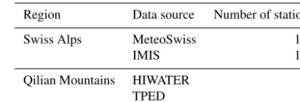
The observational mean daily air temperatures (Tobs) from the Swiss Alps and the Qilian Mountains are used for de-riving model parameters and for evaluating results (Table 1, Fig. 1). Observation datasets from the Swiss Alps were obtained from the MeteoSwiss automatic monitoring net-work (184 stations) and from the Inter-cantonal Measure-ment and Information System (IMIS) at the WSL Institute for Snow and Avalanche Research SLF (178 stations). In the Qilian Mountains, there are 30 stations from the Heihe Watershed Allied Telemetry Experimental Research (HI-WATER) and 3 stations from the Third Pole Environment Database (TPED) (Li et al., 2013). Temperatures are ob-served by automatic meteorological stations using intervals from 10 to 30 min. The temperature from MeteoSwiss is observed using the Thygan instrument which has an accu-racy of±0.01◦C, and temperatures from IMIS are measured by several different sensors (including Rotronic MP100H, Rotronic MP102H/HC2, Rotronic MP103A and Campbell Scientific CS215), with sensor accuracies ranging from±0.1 to ±0.9◦C. In the Qilian Mountains, temperature sensors HMP155 with a typical accuracy of±0.2◦C are used. The 395 stations used cover an elevation range of∼250–4150 m as well as different topographic positions including peaks, slopes, plains and deep valleys (Fig. 2a).
All temperature observations were filtered using a thresh-old (plausible values from−60 to 60◦C), and the outliers of
Figure 1.Location of experimental region(a): observation stations in the Swiss Alps(b)and the Qilian Mountains(c).
Figure 2.Elevation distribution of observation station(a)and number of observation stations (N) used in different years(b).
3.3 DEM
The fine-scale topography was represented using a DEM with a resolution of 3 arcsec (∼90 m). To avoid the noise in the original dataset, the DEM used in this study was aggre-gated from the original Global Digital Elevation Model ver-sion 2 (GDEM2) with a grid spacing of 1 arcsec (Tachikawa et al., 2011; Meyer et al., 2011) to a spacing of 3 arcsec by averaging (Fig. B1 in Appendix B).
4 Methods
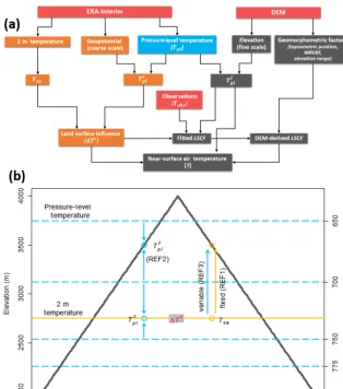
Figure 3 shows a flowchart (a) and schematic illustration (b) of REDCAPP. The main steps can be summarized as (1) ob-tainingTsa and interpolatingTplc andTplf from the pressure-level data (described in Sect. 4.1); (2) deriving 1Tc=
Figure 3.Model flow chart(a)and schematic illustration of interpolations and reference methods(b). Red squares denote input datasets. Variables at the elevation of coarse-scale topography are marked in yellow while the elevation of fine-scale topography is shown in grey.Tpl in blue could be at both the coarse and fine scales of elevation. Blue arrows and points are variable lapse rates and temperatures derived from
Tpl, while the yellow point is temperature derived fromTsa, and the yellow arrow is the fixed lapse rate of−6.5◦C km−1. Detailed symbol and variable names can be found in Appendix A. The schematic illustration is revised from Fiddes and Gruber (2014).
The fundamental of REDCAPP is coupling the1T to the Tplat each site and could be given by
T =Tpl+1T , (1)
whereTplis the air temperature of pressure level from ERA-Interim, and1T is the influence of land surface. In response to the required fine scale ofT, Eq. (1) could be changed to
T =Tplf+1Tf, (2)
whereTplf and1Tfis theTpland1T at the elevation of fine-scale topography.
4.1 Interpolation of air temperature
By following Fiddes and Gruber (2014), Tplf and Tplc at a given site are obtained by 3-D interpolation of Tpl. This is achieved in two steps: (1) 2-D interpolation: deriving the el-evation of each pressure level by normalizing geopotential
height (Eq. 3) and then conducting horizontal 2-D interpo-lation of temperature and elevation for each pressure level; (2) 1-D interpolation: vertically interpolatingTplat different heights over one location to the required elevation.
Elevation= φ
g0
4.2 Land-surface correction factor
The land-surface effect 1Tc on simulated near-surface air temperature is given by
1Tc=Tsa−Tplc. (4)
LSCF is introduced here as a scale factor to obtain1Tffrom 1Tc. Therefore, Eq. (2) becomes
Tf=Tplf+LSCF·1Tc, (5)
where LSCF describes the effect of fine-scale topography on the relative magnitude of land-surface effects. It is parame-terized as
LSCF=α·h+β·v, (6)
whereα,β are positive numbers obtained from fitting with observations, andhandv [0,1] are factors derived heuristi-cally from geomorphology on the fine-scale topography. The lowercase variables ofhandvare derived by scaling hypso-metric position (H) and the degree of valleyness (V) with a scaling factor
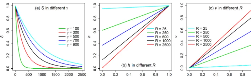
S=exp(−R
γ ), (7)
whereRis the elevation range in a prescribed neighborhood of analysis andγ is a fitting parameter. This scaling reflects the fact that stronger topographic effects on air temperature are to be expected with increasing elevation range.Sis equal to 1 forR=0 and 0 for very largeRvalues (Fig. 4a).
Hypsometric position H, the basis for h, is the ratio of the number of cells with higher elevation than a given site to the total number of cells in a prescribed neighborhood of analysis. It ranges from 1 (deepest valley) to 0 (highest peak). The prescribed neighborhood of analysis for bothH and R is taken as 30 km×30 km. For computational effi-ciency,His derived based on a DEM aggregated to 15 arcsec (∼450 m) by averaging and the results are nearly identical (Appendix B1). Then,His scaled to obtain
h=H·(1−S)+S. (8)
The lowest point in the landscape thus always receives a weight of 1 inh(Fig. 4b).
The factorvis based on scaling a measure of the degree of valleyness [0,1]:
v=V·(1−S), (9)
where v becomes larger with increasing elevation range (Fig. 4c) and V is described by the normalized multireso-lution valley bottom flatness (MRVBF) index (Gallant and Dowling, 2003):
V = MRVBF
MRVBFmax
, (10)
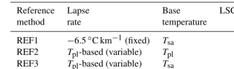
Table 2.Summary of reference methods.
Reference Lapse Base LSCF method rate temperature
REF1 −6.5◦C km−1(fixed) Tsa 1 REF2 Tpl-based (variable) Tpl 0 REF3 Tpl-based (variable) Tsa 1
REF2 is from Fiddes and Gruber (2014), while REF3 is from Gao et al. (2012).
where MRVBF identifies valley bottoms occurring at a range of scales (Gallant and Dowling, 2003), and MRVBFmax is a constant value of 8 based on the maximum MRVBF. The original slope threshold used to scale flatness of topogra-phy is increased to 50 % in this study, so that the MRVBF is smoother (Appendix B2).
The main parameters for REDCAPP, denoted by the greek lettersα, β and γ, are derived from fitting with observa-tional data. For this, values for LSCF were fitted where ob-servations exist. Then, model parameters for predicting these LSCFs were derived using global optimization function “dif-ferential_evolution” of the Python package SciPy (Storn and Price, 1997).
4.3 Reference methods
Three reference methods using different sources of air tem-perature and lapse rate are used to compare with the new downscaling scheme (Table 2, Fig. 3). Tsa is extrapolated by using a fixed lapse rate of−6.5◦C km−1(REF1) and by using variable lapse rate modeled fromTpl(REF3) (Giorgi et al., 2003; Gao et al., 2012). Linearly interpolatedTpl is referenced as REF2 (Fiddes and Gruber, 2014; Gupta and Tarboton, 2016). Since only the upper-air temperatures are used in REF2, this is equivalent to setting LSCF uniformly to 0 (no land-surface influence), while LSCF is uniformly considered to be 1 in REF1 and REF3, which useTsaas their base temperature. To evaluate the performance of REDCAPP against the three reference methods, the coefficient of deter-mination (R2), root mean squared error (RMSE) and mean bias (BIAS) were computed here.
RMSE= v u u u t N P
t=1
(OBSt−MODt)2
N (11)
BIAS= 1
N N X
t=1
(MODt−OBSt) (12)
5 Results
Figure 4. (a)Scale factor (S) decreases with increasing elevation range (R) by using differentγ values. Fraction influence of surface effect on T (h) increases with hypsometric position (H) and strength of CAP (v) increases with the normalized multiresolution valley bottom flatness (V).γis 500 in panels(b, c). The lowest point in the landscape always receives a weight of 1 inhand a weight of 0 inv.
Figure 5.Seasonal changes shown as monthly distributions of average daily1Tcderived from ERA-Interim for the locations of all stations. Red dots are median values.
1T and whether it can be used for parameterizing cold air pooling and surface effects. Then, we investigate LSCF and its estimation based on a fine-scale DEM. Finally, the perfor-mance of REDCAPP is evaluated.
5.1 Properties of1T
Figure 5 presents seasonal variations of daily1Tc. In gen-eral,1Tcis close to 0◦C in warm seasons with the median value sightly above 0◦C in the Swiss Alps from March to June and greater than−0.8◦C in the Qilian Mountains from April to June. In winter, lower median1Tcvalues are found in both the Swiss Alps and the Qilian Mountains. Further-more, a larger range of 1Tc in winter is caused by lower minima of1Tc, likely related to radiative cooling.
Figure 6 shows one year of daily 1Tc as well as T de-rived from observations and downscaling at selected sites. The downscaled series are either ignoring 1Tc (REF2) or adding it uniformly (REF3) to all stations. Daily1Tcshows a similar pattern to Fig. 5. At the mountain sites (COV, BEV1, DDS; see Table 3), Tplf describesTobs well without accounting for1Tc(REF2), and the RMSEs were less than 1.4◦C (Table 3). By contrast, REF2 does not describeTobs well at valley locations, especially in winter, and RMSEs are
markedly higher. In comparison, the results of REF3, through adding1Tc toTplf, followTobs better at valley sites (SAM, SIA, EBO) and worse at mountain sites. Although REF3 im-proves predictions in deep valleys (e.g., SAM), results in winter are still higher than the observations because winter inversions here are stronger than predicted by1Tc.
These results highlight the spatial and temporal variability of land-surface effects onT. As the full incorporation of1Tc in downscaling improves predictions in valley locations and degrades them in mountain sites, a spatially variable LSCF appears to be a promising means for better predicting land-surface effects onT at the fine scale.
5.2 Land-surface correction factor
Figure 6.Detailed time series of1Tc,Tobs, REF2 and REF3 at the selected stations from different geomorphometric positions.
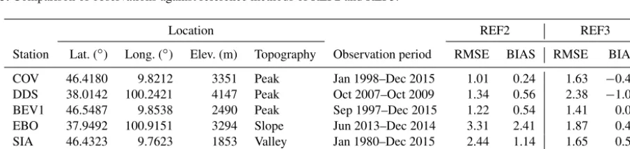
Table 3.Comparison of observations against reference methods of REF2 and REF3.
Location REF2 REF3
Station Lat. (◦) Long. (◦) Elev. (m) Topography Observation period RMSE BIAS RMSE BIAS COV 46.4180 9.8212 3351 Peak Jan 1998–Dec 2015 1.01 0.24 1.63 −0.41 DDS 38.0142 100.2421 4147 Peak Oct 2007–Oct 2009 1.34 0.56 2.38 −1.05 BEV1 46.5487 9.8538 2490 Peak Sep 1997–Dec 2015 1.22 0.54 1.41 0.04 EBO 37.9492 100.9151 3294 Slope Jun 2013–Dec 2014 3.31 2.41 1.87 0.43 SIA 46.4323 9.7623 1853 Valley Jan 1980–Dec 2015 2.44 1.14 1.65 0.50 SAM 46.5263 9.8789 1756 Valley Jan 1980–Dec 2015 3.85 1.95 2.81 1.39
LSCFs greater than 0 hint at the possibility of representing CAPs by using a LSCF and1Tc.
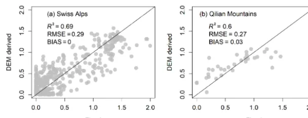
To assess the performance of DEM-derived LSCF (based on Eq. 5), we conducted a 10-fold cross validation separately for the Swiss Alps and the Qilian Mountains (Fig. 8). Each time, ∼90 % of the observations are randomly selected for deriving model parameters and the remaining 10 % are used for evaluation. Results show an RMSE of 0.29 and 0.26, a BIAS of 0 and 0.03, as well as an R2 of 0.69 and 0.60 in the Swiss Alps and the Qilian Mountains. These results in-dicate that LSCF can be estimated from a DEM based on
geomorphometry and that results will be useful in improving downscaling.
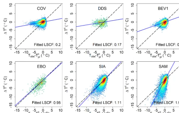
Figure 7.Difference of observed temperature and a prediction involving pressure levels (Tobs−Tplf) against1Tc. The representation is a smoothed color density of a scatter plot to make a quantity of points visual. The lines are results of LSCF×1Tcby using LSCF of 1 (black dash) and best-fitted LSCF (blue solid) at the selected stations. The time periods of the stations are presented in Table 3.
Table 4.Summary of model parameters for estimating LSCF from DEMs.
Area Model parameters Evaluation
α β γ R2 RMSE BIAS
Swiss Alps 0.61±0.03 1.56±0.04 465±50 0.69 0.29 0.00 Qilian Mountains 0.90±0.08 0.34±0.11 138±20 0.68 0.26 0.03
The values after±are standard deviations derived from 10-fold cross validation.
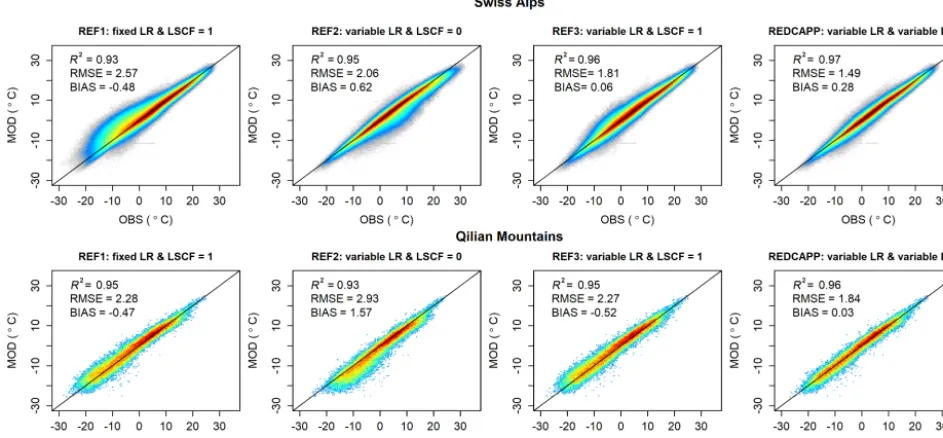
5.3 Performance of REDCAPP 5.3.1 Comparison with station data
Figure 10 shows plots ofTobsagainst results of REF1, REF2, REF3 and REDCAPP (MOD), and indicates that REDCAPP improves the prediction of T over reference methods. The downscaled results achieve better measures of agreements or reduce deviance by comparing the references methods. This is because REF3 resulted in air temperatures being too low at high elevation, while the influence of CAP was underesti-mated in valleys by applying a fixed LSCF of 1 to the entire area. As a result, the BIAS of REF3 is very close to 0 due to differing biases canceling out each other.
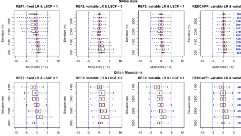
Figure 11 shows the seasonal deviance of downscaled daily results (MOD–OBS) for different methods. Similar to the detailed comparison of typical stations showed in Fig. 6, REF2 captures temperatures in summer well but has a warm bias in winter. By contrast, REF1 predictsT too low in win-ter. This is because the lapse rates are expected to increase due to the presence of CAPs. There is no obvious seasonal trend in the median deviation of REF3. However, the mini-mum of deviation is smaller than REF2 in winter. REDCAPP capturesT well in both winter and summer. The median
de-viation for each month was within±0.50◦C (from−0.06 to 0.48◦C) in the Swiss Alps and within±0.55◦C (from−0.53 to 0.45◦C) in the Qilian Mountains.
Figure 12 shows the deviances of downscaled results by elevation. REF2 performs well at high-elevation areas, with the median deviance close to 0, but has a warm bias with decreasing elevation. By contrast, REF1 and REF3 tend to have a cold bias at high elevation and often an increasing range of deviance with elevation. REDCAPP capturesT well across elevations. The median deviance was within±0.70 (from−0.24 to 0.68)◦C in the Swiss Alps and within±1.25 (from−0.76 to 1.22)◦C in the Qilian Mountains.
Figure 8.A 10-fold cross validation of DEM-derived LSCF against fitted values in the Swiss Alps(a)and the Qilian Mountains(b).
Figure 9.Spatial variation of elevation(a), hypsometric position(b), normalized MRVBF(c)and LSCF(d)in selected slope terrain.
5.3.2 Spatial signature of REDCAPP
Figure 14 shows the spatial variation of mean annual1Tffor the year 2015. In valleys, downscaledT can be up to−2.1◦C
lower thanTplf. With increasing elevation, the simulated land-surface effect decreased to almost 0◦C. This gives a clear picture on the topography-related spatial variability of1Tf and indicates REDCAPP can capture the variations well.
6 Discussion
In this section, we discuss advantages and limitations of the model and how it could be further refined in the future. We have demonstrated that information from coarse-scale mod-els (1Tc) can be used as a proxy of land-surface effects and, with a disaggregation factor (LSCF) estimated from a fine-scale DEM, can improve air temperature downscaling in mountains. At the same time, this finding needs to be put into perspective: a full simulation of the atmospheric physics and land surface at high resolution will likely outperform this pa-rameterization but at a cost that is orders of magnitude higher (Fowler et al., 2007). Ultimately, the choice of method (or combination of several methods) depends on the problem at hand. It is likely that the parameterization put forward here can be further improved in its ability to predict fine-scale pat-terns and its suitability for transferring parameters between
areas and thus the suitability for application in data-sparse regions. Nevertheless, REDCAPP and similar methods (Fid-des et al., 2015; Gupta and Tarboton, 2016) demonstrate that coarse-scale information on atmospheric variables can con-tribute to better prediction at finer scales without the need for increased resolution in the atmospheric model.
6.1 Comparison with other downscaling techniques Though the upper-air temperatures (Tplf andTplc) are obtained following Fiddes and Gruber (2014), disaggregating the dif-ference of upper-air and near-surface temperatures as a proxy of surface effects (1T) makes REDCAPP a new method. Additionally, the1T in REDCAPP is adjusted to fine scale in response to the spatial heterogeneity of surface effect based on LSCF derived from DEM and observations, rather than ignored (REF2) or treated as spatially invariant (REF1 and REF3).
Figure 10.Tobs(OBS) against results of REF1, REF2, REF3 and REDCAPP (MOD). LR in the subtitles indicates lapse rate.
Figure 11.Seasonal deviance of downscaled daily results (MOD–OBS) for different methods. Red dots are median values.
ofT with geographic (e.g., slopes, coastal) and meteorologi-cal (e.g., atmosphere boundary layer) factors . Similarly, the approach by Thornton et al. (1997) calculates interpolation weights for the stations nearby and corrects the downscaled results based on an empirical relationship ofT to elevation, and Hijmans et al. (2005) conducted a second-order spline interpolation using latitude, longitude and elevation as in-dependent variables. As observations are usually sparse in mountains, especially at higher elevation, these methods are expected to have significant uncertainty caused by inade-quate sampling of elevation and hence lapse rate. In
compar-ison, REDCAPP relies on reanalysis data for air temperature and uses station data only for calibration of the LSCF related to CAP. REDCAPP derives lapse rates from multiple layers of upper-air temperature encompassing the entire elevation range of study area. Thus, REDCAPP results are expected to be robust because both theTsa andTpl from reanalysis are used.
6.2 Land-surface correction factor
Figure 12.Deviances of downscaled results by elevations. The stations are grouped by elevation with an interval of 300 m. Each box may contain multiple stations and the numbers of observation times (days) are given in blue on the right. Red dots are median values.
but is constant over time. This lumped nature of LSCF is imperfect because the presence of strong valley inversion in winter and their absence in the warm season would suggest a seasonally variable LSCF. In other words, LSCF is expected to be greater in winter than in summer as the fractional influ-ence of CAP (the part ofβin Eq. 6) should be removed from LSCF. In REDCAPP, applying the same LSCF year-round to1Tcwill make downscaledT higher in winter and lower in summer. A potential avenue for addressing this problem is simulating the likelihood for CAPs based on surface net radiation or Richardson number based on the reanalysis data. 6.3 Transferability
Based on the 10-fold cross validation, LSCF is modeled well in both the Swiss Alps and the Qilian Mountains. The result-ing parameter values, however, are different (Table 4). The reasons for this can be speculated to include differences in topography (e.g., valley shape), the number and distribution of stations used, climate (continentality, effect of lumping two processes into one LSCF) or differences in land-surface characteristics (e.g., canopy and snow cover). The differ-ence in estimated parameter values of LSCF limits the direct transferability of REDCAPP parameters from the mountains tested here to others, as it requires new calibration in other mountain regions. This is a significant drawback and we hope that over time, application in many mountain ranges will help to establish correlations of trusted parameter values with
en-vironmental conditions. REDCAPP can be applied to other mountains once the parameters (α,β andγ in Eqs. 6 and 7) of LSCF are derived based on observations and a fine-scale DEM.
6.4 Input data
Although we only apply and test our method with ERA-Interim here, it can be used with other reanalyses such as CFSR, NCEP, MERRA or 20CRV2. Besides global re-analyses, regional high-resolution assimilations produced by RCMs (e.g., E-OBS, Chinese Academy of Sciences forcing data, ASR) (Chen et al., 2011), and upper-air temperature analyses (e.g., ASR) may be suitable alternatives in some re-gions. These regional assimilations often capture surface air temperature better by assimilating more observations and by using finer grids than global reanalyses. Since upper-air tem-perature and1T are treated separately in REDCAPP, they can also be derived from different data sources.
6.5 Future development
Figure 13.Comparison of REF2, REF3 and REDCAPP with time series at selected stations. The daily temperatures present are averaged based on all available years (Table 3); the shorter time series for EBO explains the larger variation in the plot.
Figure 14.The fine scale of land-surface influence (1Tf) for the test area.
surface conditions (e.g., snow, canopy, soil moisture), which are considered important (Lin et al., 2016; Liston and Elder, 2006).
7 Conclusions
We describe and test a downscaling method for near-surface air temperature. It derives1T from coarse-scale atmospheric model data as a proxy of the effect that the land surface has on near-surface air temperature. The magnitude of this effect is adjusted at the fine scale based on geomorphometric
char-acteristics derived from a fine scale of a DEM. The results from the new method are evaluated with 395 stations in two mountain ranges, leading to these conclusions:
1. The proxy1T is suitable for parameterizing CAP and surface effects.
2. The land-surface correction factor LSCF can be pre-dicted from a fine-scale DEM where∼70 % of the vari-ance in directly fitted LSCF could be explained by the parameterization.
3. REDCAPP improves downscaling when compared with reference methods. This is primarily because the advan-tages of REF2 and REF3 are combined.
4. The transfer of REDCAPP parameters between moun-tain ranges is difficult and at present, separate fitting pa-rameters in new regions are recommended.
REDCAPP can produce daily, high-resolution (here
∼90 m) gridded fields of near-surface air temperature in mountains. This can provide input for other models simu-lating phenomena related to, e.g., hydrology, permafrost and ecology. The input data are not limited to ERA-Interim and could be extended to other reanalyses such as CFSR, NCEP, MERRA or 20CRV2.
Appendix A: Nomenclature
In this study, T refers to air temperatures, subscripts iden-tify the source (obs: observation; sa: surface analysis; pl: pressure level) and superscripts identify the elevation (c: coarse scale, f: fine scale). Coarse-scale elevation refers to the topography used by the reanalysis; fine-scale refers to the DEM used for downscaling. Observations refer to mean daily air temperature and are assumed to be at the elevation of fine-scale topography. The surface analysis fields in the reanalysis are given at the elevation of the coarse-scale topography (as obtained from invariant geopotential ERA-Interim file by Eq. 3); pl represents air temperature derived from pressure levels and can be either. The following list provides the definitions of symbols for REDCAPP.
Symbol Name Unit
T Near-surface air temperature ◦C
Tobs Observational surface air temperature ◦C
Tsa 2 m air temperature at the elevation of coarse scale ◦C
Tpl Air temperature of pressure level in reanalysis, known as upper-air temperature ◦C Tplc Air temperature of pressure level at the elevation of coarse scale ◦C Tplf Air temperature of pressure level at the elevation of fine scale ◦C
1T Land-surface influences on surface air temperature ◦C
1Tc Land-surface influences on surface air temperature at elevation of coarse scale ◦C 1Tf Land-surface influences on surface air temperature at elevation of fine scale ◦C
LSCF Land-surface correction factor –
α Fractional influence of surface effects on air temperature –
β Influences of cold air pooling on air temperature –
h Scaled hypsometric position –
H Hypsometric position –
v Degree of valleyness –
MRVBF Multiresolution valley bottom flatness index –
V Normalized multiresolution valley bottom flatness index –
B2 Multiresolution index of valley bottom flatness The choice of suitable parameters for MRVBF is affected by the resolution of the input DEM as well as different land-scape characteristics and applications (Gallant and Dowl-ing, 2003). In response to the cold air pooling movement, the slope threshold is adjusted from the original value of 16 to 50 % in this study. Figure B3 compares MRVBF using a slope threshold of 50 and 16 % (original paper) in the Alps and the Qilian Mountains. The results indicate that MRVBF is smoother when using the larger threshold and hence likely describes cold air movement better. The threshold value of 50 was chosen after considerable tests and comparisons but ultimately remains a subjective choice at this time.
Figure B2.Comparison of hypsometric position derived from coarse-scale (15 arcsec) and fine-scale (3 arcsec) DEMs based on a random sample of 1000 points.
Competing interests. The authors declare that they have no conflict of interest.
Acknowledgements. We would like to express our gratitude to John C. Gallant for his help with the multiresolution index of valley bottom flatness. Station data in Switzerland are provided by the Swiss Federal Office of Meteorology and Climatology (Me-teoSwiss) and Inter-cantonal Measurement and Information System (IMIS) from the WSL Institute for Snow and Avalanche Research SLF. The authors would like to thank Joel Fiddes for help with the IMIS dataset. We would also like to thank the Heihe Watershed Allied Telemetry Experimental Research (HIWATER) project and Third Pole Environment Database for providing air temperature in the Qilian Mountains. We thank ECMWF for the ERA-Interim reanalysis data. This study was supported by the National Natural Science Foundation of China (91325202), the National Key Scien-tific Research Program of China (2013CBA01802), partly by the Fundamental Research Funds for the Central Universities (China) and by the projected of “Quantifying the Hidden Thaw” funded by the Canada Foundation for Innovation (CFI). The ASTER dataset is downloaded from http://gdex.cr.usgs.gov/gdex/.
Edited by: Patrick Jöckel
Reviewed by: two anonymous referees
References
Bao, X. and Zhang, F.: Evaluation of NCEP-CFSR, NCEP-NCAR, ERA-Interim, and ERA-40 Reanalysis Datasets against Indepen-dent Sounding Observations over the Tibetan Plateau, J. Climate, 26, 206–214, https://doi.org/10.1175/JCLI-D-12-00056.1, 2013. Berrisford, P., Dee, D., Poli, P., Brugge, R., Fielding, K., Fuentes, M., Kallberg, P., Kobayashi, S., Uppala, S., and Simmons, A.: The ERA-Interim archive, version 2.0, Technical report, ECMWF, 2011.
Bürger, G., Murdock, T. Q., Werner, A. T., Sobie, S. R., and Cannon, A. J.: Downscaling Extremes – An Intercomparison of Multiple Statistical Methods for Present Climate, J. Climate, 25, 4366– 4388, https://doi.org/10.1175/JCLI-D-11-00408.1, 2012. Chen, G., Iwasaki, T., Qin, H., and Sha, W.: Evaluation
of the Warm-Season Diurnal Variability over East Asia in Recent Reanalyses JRA-55, ERA-Interim, NCEP CFSR, and NASA MERRA, J. Climate, 27, 5517–5537, https://doi.org/10.1175/JCLI-D-14-00005.1, 2014.
Grant, A. N., Groisman, P. Y., Jones, P. D., Kruk, M. C., Kruger, A. C., Marshall, G. J., Maugeri, M., Mok, H. Y., Nordli, Ø., Ross, T. F., Trigo, R. M., Wang, X. L., Woodruff, S. D., and Worley, S. J.: The Twentieth Century Reanalysis Project, Q. J. Roy. Me-teor. Soc., 137, 1–28, https://doi.org/10.1002/qj.776, 2011. Daly, C.: Guidelines for assessing the suitability of
spa-tial climate data sets, Int. J. Climatol., 26, 707–721, https://doi.org/10.1002/joc.1322, 2006.
Daly, C., Taylor, G. H., Gibson, W. P., Parzybok, T. W., Johnson, G. L., and Pasteris, P. A.: High-quality spatial climate data sets for the United States and beyond, T. ASAE, 43, 1957–1962, 2000.
Daly, C., Gibson, W., Taylor, G., Johnson, G., and Pasteris, P.: A knowledge-based approach to the statistical mapping of climate, Clim. Res., 22, 99–113, https://doi.org/10.3354/cr022099, 2002. Dee, D. P., Uppala, S. M., Simmons, A. J., Berrisford, P., Poli, P., Kobayashi, S., Andrae, U., Balmaseda, M. A., Balsamo, G., Bauer, P., Bechtold, P., Beljaars, A. C. M., van de Berg, L., Bid-lot, J., Bormann, N., Delsol, C., Dragani, R., Fuentes, M., Geer, A. J., Haimberger, L., Healy, S. B., Hersbach, H., Hølm, E. V., Isaksen, L., Kållberg, P., Köhler, M., Matricardi, M., McNally, A. P., Monge-Sanz, B. M., Morcrette, J.-J., Park, B.-K., Peubey, C., de Rosnay, P., Tavolato, C., Thépaut, J.-N., and Vitart, F.: The ERA-Interim reanalysis: configuration and performance of the data assimilation system, Q. J. Roy. Meteor. Soc., 137, 553–597, https://doi.org/10.1002/qj.828, 2011.
Dimri, A. P.: Impact of subgrid scale scheme on topography and lan-duse for better regional scale simulation of meteorological vari-ables over the western Himalayas, Clim. Dynam., 32, 565–574, https://doi.org/10.1007/s00382-008-0453-z, 2009.
Fiddes, J. and Gruber, S.: TopoSCALE v.1.0: downscaling gridded climate data in complex terrain, Geosci. Model Dev., 7, 387–405, https://doi.org/10.5194/gmd-7-387-2014, 2014.
Fiddes, J., Endrizzi, S., and Gruber, S.: Large-area land surface sim-ulations in heterogeneous terrain driven by global data sets: ap-plication to mountain permafrost, The Cryosphere, 9, 411–426, https://doi.org/10.5194/tc-9-411-2015, 2015.
Fowler, H. J., Blenkinsop, S., and Tebaldi, C.: Linking climate change modelling to impacts studies: recent advances in down-scaling techniques for hydrological modelling, Int. J. Climatol., 27, 1547–1578, https://doi.org/10.1002/joc.1556, 2007. Gallant, J. C. and Dowling, T. I.: A multiresolution index of valley
bottom flatness for mapping depositional areas, Water Resour. Res., 39, 1347, https://doi.org/10.1029/2002WR001426, 2003. Gao, L., Bernhardt, M., and Schulz, K.: Elevation correction of
Syst. Sci., 16, 4661–4673, https://doi.org/10.5194/hess-16-4661-2012, 2012.
Giorgi, F., Francisco, R., and Pal, J.: Effects of a Subgrid-Scale Topography and Land Use Scheme on the Simu-lation of Surface Climate and Hydrology. Part I: Effects of Temperature and Water Vapor Disaggregation, J. Hy-drometeorol., 4, 317–333, https://doi.org/10.1175/1525-7541(2003)4<317:EOASTA>2.0.CO;2, 2003.
Gruber, S.: Derivation and analysis of a high-resolution estimate of global permafrost zonation, The Cryosphere, 6, 221–233, https://doi.org/10.5194/tc-6-221-2012, 2012.
Gupta, A. S. and Tarboton, D. G.: A tool for downscaling weather data from large-grid reanalysis products to finer spatial scales for distributed hydrological applications, Environ. Model. Softw., 84, 50–69, https://doi.org/10.1016/j.envsoft.2016.06.014, 2016. Hagemann, S., Machenhauer, B., Jones, R., Christensen, O. B.,
Déqué, M., Jacob, D., and Vidale, P. L.: Evaluation of water and energy budgets in regional climate models applied over Europe, Clim. Dynam., 23, 547–567, https://doi.org/10.1007/s00382-004-0444-7, 2004.
Harris, I., Jones, P., Osborn, T., and Lister, D.: Updated high-resolution grids of monthly climatic observations – the CRU TS3.10 Dataset, Int. J. Climatol., 34, 623–642, https://doi.org/10.1002/joc.3711, 2014.
Hay, L. and Clark, M.: Use of statistically and dynamically downscaled atmospheric model output for hydrologic simu-lations in three mountainous basins in the western United States, J. Hydrol., 282, 56–75, https://doi.org/10.1016/S0022-1694(03)00252-X, 2003.
Hijmans, R. J., Cameron, S. E., Parra, J. L., Jones, P. G., and Jarvis, A.: Very high resolution interpolated climate sur-faces for global land areas, Int. J. Climatol., 25, 1965–1978, https://doi.org/10.1002/joc.1276, 2005.
Hodges, K. I., Lee, R. W., and Bengtsson, L.: A Comparison of Ex-tratropical Cyclones in Recent Reanalyses ERA-Interim, NASA MERRA, NCEP CFSR, and JRA-25, J. Climate, 24, 4888–4906, https://doi.org/10.1175/2011JCLI4097.1, 2011.
Hofer, M., Mölg, T., Marzeion, B., and Kaser, G.: Empirical-statistical downscaling of reanalysis data to high-resolution air temperature and specific humidity above a glacier sur-face (Cordillera Blanca, Peru), J. Geophys. Res.-Atmos., 115, d12120, https://doi.org/10.1029/2009JD012556, 2010.
Jones, P. and Kelly, P.: The spatial and temporal characteristics of Northern Hemisphere surface air temperature variations, J. Cli-matol., 3, 243–252, 1983.
Kiefer, M. T. and Zhong, S.: The role of forest cover and valley geometry in cold-air pool evolution, J. Geophys. Res.-Atmos., 120, 8693–8711, https://doi.org/10.1002/2014JD022998, 2015. Kistler, R., Collins, W., Saha, S., White, G., Woollen, J., Kalnay, E.,
Chelliah, M., Ebisuzaki, W., Kanamitsu, M., Kousky, V., van den Dool, H., Jenne, R., and Fiorino, M.: The NCEP–NCAR 50-Year Reanalysis: Monthly Means CD-ROM and Documentation, B. Am. Meteorol. Soc., 82, 247–267, https://doi.org/10.1175/1520-0477(2001)082<0247:TNNYRM>2.3.CO;2, 2001.
Lareau, N. P., Crosman, E., Whiteman, C. D., Horel, J. D., Hoch, S. W., Brown, W. O. J., and Horst, T. W.: The Persis-tent Cold-Air Pool Study, B. Am. Meteorol. Soc., 94, 51–63, https://doi.org/10.1175/BAMS-D-11-00255.1, 2013.
Lewkowicz, A. G. and Bonnaventure, P. P.: Equivalent Elevation: A New Method to Incorporate Variable Surface Lapse Rates into Mountain Permafrost Modelling, Permafrost Periglac., 22, 153– 162, https://doi.org/10.1002/ppp.720, 2011.
Li, X., Cheng, G., Liu, S., Xiao, Q., Ma, M., Jin, R., Che, T., Liu, Q., Wang, W., Qi, Y., Wen, J., Li, H., Zhu, G., Guo, J., Ran, Y., Wang, S., Zhu, Z., Zhou, J., Hu, X., and Xu, Z.: Heihe Wa-tershed Allied Telemetry Experimental Research (HiWATER): Scientific Objectives and Experimental Design, B. Am. Mete-orol. Soc., 94, 1145–1160, https://doi.org/10.1175/BAMS-D-12-00154.1, 2013.
Lin, P., Wei, J., Yang, Z.-L., Zhang, Y., and Zhang, K.: Snow data assimilation-constrained land initialization improves sea-sonal temperature prediction, Geophysical Res. Lett., 43, 11423– 11432, https://doi.org/10.1002/2016GL070966, 2016.
Liston, G. E. and Elder, K.: A Meteorological Distribution Sys-tem for High-Resolution Terrestrial Modeling (MicroMet), J. Hydrometeorol., 7, 217–234, https://doi.org/10.1175/JHM486.1, 2006.
Lundquist, J. D. and Cayan, D. R.: Surface temperature patterns in complex terrain: Daily variations and long-term change in the central Sierra Nevada, California, J. Geophys. Res-.Atmos., 112, d11124, https://doi.org/10.1029/2006JD007561, 2007.
Mahrt, L., Vickers, D., Nakamura, R., Soler, M. R., Sun, J., Burns, S., and Lenschow, D.: Shallow Drainage Flows, Bound.-Lay. Meteorol., 101, 243–260, https://doi.org/10.1023/A:1019273314378, 2001.
Maraun, D., Wetterhall, F., Ireson, A. M., Chandler, R. E., Kendon, E. J., Widmann, M., Brienen, S., Rust, H. W., Sauter, T., The-meßl, M., Venema, V. K. C., Chun, K. P., Goodess, C. M., Jones, R. G., Onof, C., Vrac, M., and Thiele-Eich, I.: Precipita-tion downscaling under climate change: Recent developments to bridge the gap between dynamical models and the end user, Rev. Geophys., 48, rG3003, https://doi.org/10.1029/2009RG000314, 2010.
Meyer, D., Tachikawa, T., Kaku, M., Iwasak, A., Gesch, D., Oimoen, M., Zhang, Z., Danielson, J., Krieger T., Curtis, B., Haase, J., Abrams, M., Crippen, R., and Carabajal, C.: ASTER Global Digital Elevation Model Version 2 – Summary of Valida-tion Results, Japan-US ASTER Science Team, 1–26, 2011. Minder, J. R., Mote, P. W., and Lundquist, J. D.: Surface
tem-perature lapse rates over complex terrain: Lessons from the Cascade Mountains, J. Geophys. Res.-Atmos., 115, d14122, https://doi.org/10.1029/2009JD013493, 2010.
Mokhov, I. I. and Akperov, M. G.: Tropospheric lapse rate and its relation to surface temperature from reanaly-sis data, Izvestiya, Atmos. Ocean. Phys., 42, 430–438, https://doi.org/10.1134/S0001433806040037, 2006.
Mugford, R. I., Christoffersen, P., and Dowdeswell, J. A.: Evalua-tion of the ERA-Interim Reanalysis for Modelling Permafrost on the North Slope of Alaska ERA-Interim Validation, in: Proceed-ings of the 10th International Conference on Permafrost, 25–29 June 2012, Salekhard, Russia, 2012.
ating surfaces of daily meteorological variables over large regions of complex terrain, J. Hydrol., 190, 214–251, https://doi.org/10.1016/S0022-1694(96)03128-9, 1997.